$BB$ Potentials in Quenched Lattice QCD

Abstract

The potentials between two $B$-mesons are computed in the heavy-quark limit using quenched lattice QCD at $m_{\pi}\sim 400~{}{\rm MeV}$. Non-zero central potentials are clearly evident in all four spin-isospin channels, $(I,s_{l})=(0,0),(0,1),(1,0),(1,1)$, where $s_{l}$ is the total spin of the light degrees of freedom. At short distance, we find repulsion in the $I\neq s_{l}$ channels and attraction in the $I=s_{l}$ channels. Linear combinations of these potentials that have well-defined spin and isospin in the $t$-channel are found, in three of the four cases, to have substantially smaller uncertainties than the potentials defined with the $s$-channel $(I,s_{l})$, and allow quenching artifacts from single hairpin exchange to be isolated. The $BB^{\ast}\pi$ coupling extracted from the long-distance behavior of the finite-volume $t$-channel potential is found to be consistent with quenched calculations of the matrix element of the isovector axial-current. The tensor potentials in both of the $s_{l}=1$ channels are found to be consistent with zero within calculational uncertainties.

I Introduction

Nuclei and nuclear processes can be described with remarkable precision by treating the nucleons as non-relativistic particles interacting via a local potential. The wealth of nucleon-nucleon (NN) scattering data has enabled the construction of precise phenomenological potentials, defined up to unitary transformations, which are used to calculate the spectra of the light nuclei. As expected from QCD, the two-body potentials alone are insufficient to reproduce the spectra, but when supplemented with three- and four- (and higher) body interactions successfully reproduce the structure of light nuclei Pieper:2001mp ; Navratil:2007we . During the last 15 years or so, immense effort has been put into developing an effective field theory (EFT) to describe the interactions between nucleons Beane:2000fx ; Bedaque:2002mn , and to allow for a systematic improvement of nuclear physics phenomenology using the approximate chiral symmetry of QCD. The values of the counterterms that appear at a given order in the EFT expansion have to be obtained from experiment or lattice QCD. In situations where experiments are not possible, lattice QCD is the only rigorous calculational technique with which to determine such counterterms. Recently, NN scattering Beane:2006mx and hyperon-nucleon scattering Beane:2006gf have been calculated with fully-dynamical lattice QCD by measuring the finite-volume shifts of two particle energies Luscher:1986pf ; Luscher:1990ux . Due to limited computational resources, the calculations were performed at unphysical pion masses, $m_{\pi}\raisebox{-3.01385pt}{$\stackrel{{\scriptstyle\textstyle>}}{{\sim}}$ }350~{}{\rm MeV}$, at the upper limits of the range of applicability of the EFTs. Until the computational resources for lattice QCD calculations are significantly greater than presently available, it will not be possible to calculate NN scattering parameters at a large number of different energies and then construct NN potentials in the same way that NN cross-section measurements are processed. However, in addition to extracting the NN phase-shifts at various moment, one can hope to learn qualitative information about the EFT describing NN interactions by performing lattice QCD calculations of systems that are similar.

In this work we study the potential between two $B^{(\ast)}$ mesons in the heavy-quark limit Isgur:1989vq ; Isgur:1989ed ; Eichten:1989zv ; Georgi:1990um  , a limit in which the potential is a well-defined object. $B$-mesons are isospin-${1\over 2}$ hadrons, and in the heavy-quark limit the spin of the light degrees of freedom (ldof) becomes a good quantum number, $s_{l}={1\over 2}$, as spin-dependent interactions with the heavy-quark are suppressed by $1/m_{b}$. At distances which are large compared with the chiral symmetry breaking scale, $\Lambda_{\chi}$, the EFT describing the interactions between two $B$-mesons is the same as that between two nucleons as the isospin-spin quantum numbers are the same. The differences between the two EFTs are in the values of the counterterms. At distances that are of order, or shorter than $\Lambda_{\chi}$ the interactions between two $B$-mesons will be arbitrarily different from that between two-nucleons as the structure of the hadrons are very different, and in particular that strong-Coulomb interaction between the heavy-quarks becomes dominant, behaving as $\sim\alpha(r^{-1})/r$ as the separation, $r\rightarrow 0$.

In addition to providing insight into the NN potential, the potentials between B-mesons are interesting in their own right. A precise determination of the potentials between two B-mesons will allow for investigations of possible shallow bound states. These would be molecular tetra-quark states, similar to the deuteron in the NN-sector. The location of such molecular states would be very sensitive to the potentials (due to the fine-tunings) and as such, quenched calculations at the unphysical pion mass would in general provide unreliable results.

Lattice calculations of the potentials between two $B$-mesons in the heavy-quark limit have been performed previously Richards:1990xf ; Mihaly:1996ue ; Stewart:1998hk ; Michael:1999nq ; Pennanen:1999xi ; Green:1999mf ; Fiebig:2001mr ; Fiebig:2001nn ; Cook:2002am ; Takahashi:2006er ; Doi:2006kx . However, given the large statistical uncertainties in those calculations, the potentials remain largely unexplored. We have chosen to work in a relatively small lattice volume in order to explore the intermediate and short-distance components of the potential, but this is at the expense of having contributions from image pairs somewhat mask the long-distance component. Further, we have attempted to extract the tensor potentials in the $s_{l}=1$ channels, but have not found results that are statistically different from zero. Due to limited computational resources, we have performed quenched calculations. It is important to stress that the long-distance component of the potential computed in quenched QCD is polluted by the presence of “one-hairpin-exchange” (OHE), as discussed in Ref. Beane:2002nu , which becomes dominant at large distances due to its exponential fall-off, as opposed to the Yukawa-type behavior of one pion exchange (OPE). However, the OHE contribution can be isolated by defining potentials with well-defined $t$-channel spin-isospin quantum numbers. In three of the $t$-channel potentials, quenching artifacts are expected to be higher order in the quenched EFT expansion. Using these finite-volume $t$-channel potentials, we are able to investigate the long range part of the infinite-volume potential and extract a $BB^{\ast}\pi$ coupling consistent with that measured in quenched lattice calculations of axial matrix elements.

The outline of our paper is as follows. In Section II, we discuss the numerical implementation of our calculation. Sections III and IV present our single particle results for the heavy hadron spectrum, including exotic states. Section V presents the main results of our work, the $BB$ potentials in the various channels. These results are then discussed in Section VI. In Appendix A, we discuss the issue of extraction of nucleon potentials from lattice QCD wavefunctions, and in Appendix B we provide details of the perturbative lattice calculations needed in this work.

II Details of the Lattice Calculation

Our calculations were performed using 284 quenched configurations of dimension $16^{3}\times 32$ generated with the DBW2 action Takaishi:1996xj ; deForcrand:1999bi for $\beta=1.04$, giving a lattice spacing of $b=0.0997\pm 0.0015$ Aoki:2002vt . On each of these configurations, eight Wilson light-quark propagators, equally spaced in the time-direction and offset in space, were generated from smeared sources to determine the light hadron spectrum. The light-quark mass selected gave rise to a pion mass of $m_{\pi}=402.5\pm 6.7~{}{\rm MeV}$, and the other hadron masses that are shown in Table. 1. The finite lattice spacing and finite-volume effects Colangelo:2003hf have not been removed from these masses and are expected to be a few percent.

	Quantity	$b\ M$	$M$ [MeV]
	$m_{\pi}$	$0.2034\pm 0.0015$	$402.5\pm 6.7$
	$m_{\rho}$	$0.3754\pm 0.0080$	$743\pm 19$
	$m_{N}$	$0.5756\pm 0.0080$	$1139\pm 23$
	$m_{\Delta}$	$0.6770\pm 0.0095$	$1340\pm 28$
	$m_{\Delta}-M_{N}$	$0.102\pm 0.014$	$201\pm 27$

Table 1: The masses of the light hadrons at finite lattice spacing and finite volume.

In order to compute the potential between two $B$-mesons separated by lattice vectors ${\bf r}=b(n,0,0),\,b(0,0,n)$ for $n=0,\ldots,8$ and additionally by ${\bf r}=b(1,1,0),\,b(2,1,0)$, Wilson light-quark propagators were generated from smeared sources on one time-slice located at each point in the $x$-$z$ plane on two adjacent spatial-slices in the y-direction on each gauge configuration. Therefore, a total of $\sim 1.4\times 10^{5}$ light-quark propagators were generated. This choice of lattice separation vectors was dictated by the available computational time, and not by physics. The calculations were performed on a 16-node dual-Xeon cluster and a number of workstations. The total computational cost of this work was $\sim$ 40 Gflop-yrs.

In the heavy-quark limit, the heavy-quark propagator is the tensor product of a Wilson line and a positive-energy projector,

$$S_{Q}({\bf x},t;t_{0})=\left(\frac{1+\gamma_{4}}{2}\right)\prod_{t^{\prime}=t_{0}}^{t}U_{4}({\bf x},t^{\prime})\,,$$ (1)

where $U_{\mu}(x)$ are the gauge link variables and the product is time-ordered. Our Dirac matrices use the Euclidean Dirac convention. The light quark propagator, $S({\bf x},t;{\bf y},t_{0})$, is generated with the unimproved Wilson action, thereby introducing ${\cal O}(b)$ discretisation errors. It is generated from a gauge-invariant Gaussian smeared-source.

To determine the single particle energies of the heavy hadrons, the correlators

$$C_{B}(t,t_{0}) = \sum_{{\bf x}}{\rm tr}\left[S_{Q}({\bf x},t;t_{0})S^{\dagger}({\bf x},t;{\bf x},t_{0})\right]\ H({\bf x})\,,$$ (2)

$$C_{\Sigma_{b}/\Lambda_{b}}(t,t_{0}) = \sum_{{\bf x}}S^{k^{\prime}k}_{Q;\sigma\rho}({\bf x},t;t_{0})\epsilon^{ijk}\epsilon^{i^{\prime}j^{\prime}k^{\prime}}\left(S^{ii^{\prime}}({\bf x},t;{\bf x},t_{0})\Gamma\right)_{\rho\alpha}\left(\Gamma S^{jj^{\prime}}({\bf x},t;{\bf x},t_{0})\right)_{\sigma\alpha}H({\bf x})\,,$$

were computed, where the Dirac matrices are $\Gamma=C\gamma_{5},\,C\gamma_{i}$ for the $\Lambda_{b}$ and $\Sigma_{b}^{i}$ respectively. The trace is over color and spinor indices, and the function $H({\bf x})$ is unity if a heavy-quark source was placed at the point ${\bf x}$, and vanishes elsewhere. In the baryon correlators, upper indices label color and lower Greek indices label spin.

In order to measure the potential, we computed the correlators $C_{I,s_{l}}(t,t_{0},\tilde{\vec{r}})$ given by

$$C_{0,0}(t,t_{0},\tilde{{\bf r}}) = \sum_{\bf x}\left[A_{0}^{(1)}-A_{0}^{(2)}\right]\ H({\bf x})\,,$$ (4)

$$C_{1,0}(t,t_{0},\tilde{{\bf r}}) = \sum_{\bf x}\left[A_{0}^{(1)}+A_{0}^{(2)}\right]\ H({\bf x})\,,$$ (5)

$$C_{0,1}(t,t_{0},\tilde{{\bf r}}) = \frac{1}{2}\sum_{\bf x}\left[A_{+}^{(1)}+A_{-}^{(1)}-A_{+}^{(2)}-A_{-}^{(2)}\right]\ H({\bf x})\,,$$ (6)

$$C_{1,1}(t,t_{0},\tilde{{\bf r}}) = \frac{1}{2}\sum_{\bf x}\left[A_{+}^{(1)}+A_{-}^{(1)}+A_{+}^{(2)}+A_{-}^{(2)}\right]\ H({\bf x})\,,$$ (7)

where

$$A_{0}^{(1)} = {\rm tr_{D}}\Big{[}{\rm tr_{C}}\left(S^{\dagger}({\bf x},t;{\bf x}+{\bf r},t_{0})S_{Q}({\bf x},t;t_{0})\right)\Gamma_{0}$$

$$\hskip 85.35826pt\times{\rm tr_{C}}\left[{\cal S}\left\{S^{\dagger}({\bf x}+{\bf r},t;{\bf x},t_{0})S_{Q}({\bf x}+{\bf r},t;t_{0})\right\}\right]^{T}\Gamma_{0}^{T}\Big{]}\,,$$

$$A_{0}^{(2)} = -{\rm tr}\Big{[}{\cal S}\left\{S^{\dagger}({\bf x},t;{\bf x}+{\bf r},t_{0})S_{Q}({\bf x}+{\bf r},t;t_{0})\right\}$$

$$\hskip 85.35826pt\times\Gamma_{0}\left[S^{\dagger}({\bf x}+{\bf r},t;{\bf x},t_{0})\right]^{T}S_{Q}({\bf x},t;t_{0})\Gamma_{0}\Big{]}\,,$$

$$A_{\pm}^{(1)} = {\rm tr}\left[\Gamma_{\pm}S_{Q}({\bf x},t;t_{0})S^{\dagger}({\bf x},t;{\bf x},t_{0})\right]$$

$$\hskip 85.35826pt\times{\rm tr}\left[\Gamma_{\pm}{\cal S}\left\{S^{\dagger}({\bf x}+{\bf r},t;{\bf x}+{\bf r},t_{0})S_{Q}({\bf x}+{\bf r},t;t_{0})\right\}\right]\,,$$

$$A_{\pm}^{(2)} = -{\rm tr}\left[S_{Q}({\bf x},t;t_{0}){\cal S}\left\{S^{\dagger}({\bf x},t;{\bf x}+{\bf r},t_{0})S_{Q}({\bf x}+{\bf r},t;t_{0})\right\}\Gamma_{\pm}S^{\dagger}({\bf x}+{\bf r},t;{\bf x},t_{0})\Gamma_{\pm}\right]\,,\hskip 19.91692pt$$ (11)

$\Gamma_{0}=\frac{1}{2}(1+\gamma_{4})\gamma_{5}$ and $\Gamma_{\pm}=\frac{1}{2}(1\pm i\gamma_{1}\gamma_{2})(1+\gamma_{4})$ and ${\rm tr_{C}}$, ${\rm tr_{D}}$ and ${\rm tr}$ indicate traces over color, spin and both. Here ${\cal S}\{\ldots\}$ indicates translation of the propagators by the lattice vector $-{\bf r}$ and the transpose ^T denotes spin transpose only. The different contributions to the various correlators, $A_{0,\pm}^{(1)}$ and $A_{0,\pm}^{(2)}$ correspond to the two contractions shown in Fig. 1.

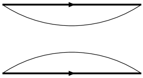
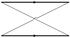
(a)                                                      (b)

Figure 1: Disconnected and connected quark contractions contributing to the correlation functions in Eqs. (4)–(7). Heavy and light lines correspond to the heavy- and light-quark propagators respectively.

For each correlator, we determine the ground state energy by seeking plateaus in the ensemble jackknife average of the effective energy,

$$b\ E_{I,s_{l}}(t-t_{0})=\log\left[\frac{C_{I,s_{l}}(t-1,t_{0})}{C_{I,s_{l}}(t,t_{0})}\right]\ .$$ (12)

III The Heavy Hadron Spectrum

In the heavy quark limit, the mass of the $B$ meson is

$$M_{B} = m_{b}\ +\ \overline{\Lambda}_{{1\over 2},{1\over 2}}\ +\ {\cal O}(1/m_{b})\ \ ,$$ (13)

where $m_{b}$ is the heavy quark mass and $\overline{\Lambda}_{I,s_{l}}$ denotes the energy of the ldof with total isospin $I$ and spin $s_{l}$. To determine $\overline{\Lambda}_{{1\over 2},{1\over 2}}$ from lattice calculations, the energy, ${\cal E}_{{1\over 2},{1\over 2}}$, of a meson composed of a Wilson-line (static color source) and a light anti-quark is computed using Eqs. (2) and (12). This by itself does not isolate $\overline{\Lambda}_{{1\over 2},{1\over 2}}$, as the interactions of the static source with the gauge fields generate a residual mass Falk:1992fm for the heavy-quark, $\delta m$, which while vanishing in dimensional regularization, is non-zero on the lattice and scales as $1/b$ with the lattice spacing Duncan:1994uq . Therefore, both ${\cal E}_{{1\over 2},{1\over 2}}$ and $\delta m$ diverge as $1/b$, but the difference between them is finite in the continuum limit, and is $\overline{\Lambda}_{{1\over 2},{1\over 2}}$,

$$\overline{\Lambda}_{{1\over 2},{1\over 2}} = {\cal E}_{{1\over 2},{1\over 2}}-\delta m\ \ \ ,$$ (14)

and more generally, $\overline{\Lambda}_{I,s_{l}}={\cal E}_{I,s_{l}}-\delta m$.

The residual mass of the static source has been computed previously out to the two-loop level in quenched lattice perturbation theory for the Wilson action Martinelli:1998vt . At the one loop level, the residual mass for a gauge action, $f$, is given by

$$\delta m_{f}^{(\alpha)} = {\overline{\alpha}(\mu)\over 3\pi^{2}b}\ \int_{-\pi}^{\pi}d\tilde{q}_{x}\ \int_{-\pi}^{\pi}d\tilde{q}_{y}\ \int_{-\pi}^{\pi}d\tilde{q}_{z}\ G_{00}^{(f)}\left(\hat{q}_{x},\hat{q}_{y},\hat{q}_{z},0\right)$$ (15)

$$= {\overline{\alpha}(\mu)\over b}\ {\cal S}^{(f)}\ \ \ ,$$

where $\hat{q}_{\gamma}=2\sin\left(\tilde{q}_{\gamma}/2\right)$, and $\tilde{q}=qb$ is dimensionless. $G_{00}^{(f)}(\hat{k}_{x},\hat{k}_{y},\hat{k}_{z},\hat{k}_{t})$ is the lattice gluon propagator for the particular gauge action, $f$. This has the form $G_{00}^{(Wilson)}(\hat{k}_{x},\hat{k}_{y},\hat{k}_{z},\hat{k}_{t})=1/{\hat{k}}^{2}$ for the Wilson action, but is considerably more complicated for improved actions, such as the Lüscher-Weisz (LW) Luscher:1984xn ; Luscher:1985zq , DBW2 Takaishi:1996xj ; deForcrand:1999bi , and Iwasaki Iwasaki actions. For these actions, the form of the propagator was presented in Ref. Weisz:1983bn and involves an improvement coefficient, $c_{1}$, with $c^{\rm LW}_{1}=-1/12$, $c^{\rm DBW2}_{1}=-1.40686$, and $c_{1}^{\rm Iwasaki}=-0.331$ (for a recent review of lattice perturbation theory, see Ref. Capitani:2002mp ). The quantity ${\cal S}^{(f)}$ has been computed previously for the Wilson action, ${\cal S}^{(Wilson)}=2.1173$, and for the improved actions we find that ${\cal S}^{(DBW2)}=0.6921$, ${\cal S}^{(LW)}=1.8335$ and ${\cal S}^{(Iwasaki)}=1.3598$ (these numbers differ from those presented in Ref. Aoki:2002iq where an incorrect improved gluon propagator was used). At the one-loop-level, the choice of scale is not well-defined, but as the only scale in the lattice calculation is the lattice spacing, it is convenient to use $\mu=1/b$. Therefore, at the one-loop level, and using $\overline{\alpha}(2~{}{\rm GeV})=0.299\pm 0.015$ , we have $\delta m^{(\alpha)}_{\rm DBW2}=410\pm 21~{}{\rm MeV}$ for the DBW2 action.

One can make an improved estimate of the residual mass term by using the Brodsky-Lepage-Mackenzie (BLM) scale-setting procedure Brodsky:1982gc , which includes the part of the two-loop contribution arising from the running of the strong coupling over the momenta in the one-loop diagram. This BLM improved residual mass is given by

$$\delta m_{f}^{(\alpha+\alpha^{2}\beta)} = {\overline{\alpha}(\mu)\over b}\ {\cal S}^{(f)}\ -\ {\overline{\alpha}^{2}(\mu)\beta\over 4\pi b}\ {\cal T}^{(f)}(\mu)\,,$$ (16)

where

$${\cal T}^{(f)}(\mu) = {1\over 3\pi^{2}}\int_{-\pi}^{\pi}d\tilde{q}_{x}\ \int_{-\pi}^{\pi}d\tilde{q}_{y}\ \int_{-\pi}^{\pi}d\tilde{q}_{z}\ G_{00}^{(f)}\left(\hat{q}_{x},\hat{q}_{y},\hat{q}_{z},0\right)\log\left[{\hat{q}_{x}^{2}+\hat{q}_{y}^{2}+\hat{q}_{z}^{2}\over\mu^{2}b^{2}}\right]\ \ \ ,$$ (17)

and $\beta=11$ for quenched QCD. The $\overline{\alpha}^{2}\beta$ term in Eq. (16) can be perturbatively removed by defining the BLM scale, $q^{\ast(f)}$, such that $\log\left(q^{*(f)}b\right)={\cal T}^{(f)}(b^{-1})/(2{\cal S}^{(f)})$, and therefore,

$$\delta m_{f}^{(\alpha+\alpha^{2}\beta)} = {\overline{\alpha}(q^{*(f)})\over b}\ {\cal S}^{(f)}\ \ \ .$$ (18)

For the Wilson action, we find ${\cal T}^{(Wilson)}(b^{-1})=1.562$ which produces a BLM scale $q^{*(Wilson)}=1.446/b$ that has previously been shown to accurately estimate the full two-loop result for the residual mass using the $\overline{\rm MS}$ coupling Martinelli:1998vt . For the improved actions, we find that ${\cal T}^{(DBW2)}(b^{-1})=-0.239$, which leads to $q^{*(DBW2)}=0.841/b$, ${\cal T}^{(LW)}(b^{-1})=1.121$, which leads to $q^{*(LW)}=1.358/b$ and for the Iwasaki action, ${\cal T}^{(Iwasaki)}(b^{-1})=0.437$, which leads to $q^{*(Iwasaki)}=1.174/b$. Therefore, using $\overline{\alpha}(q^{*(DBW2)})=0.326\pm 0.018$, the BLM improved estimate of the residual mass for our DBW2 lattices is $\delta m^{(\alpha+\alpha^{2}\beta)}_{\rm DBW2}=447\pm 25~{}{\rm MeV}$.

In Table 2 we present the extracted lattice energies and resultant energies of the ldof for the $B$-meson and the $\Lambda_{b}$ and $\Sigma_{b}$ heavy baryons. The effective mass ratios corresponding to these measurements are shown in Fig. 2. We have performed both correlated and uncorrelated single and double exponential fits to the correlation functions in order to extract the ground state energy and to estimate the uncertainty in the extraction. The differences between the extracted ground state energies from these procedures is encapsulated in the systematic error. The fitting range quoted in Table 2 (and all other tables) is that used in fitting a single exponential to the correlation function. The statistical errors are determined by the Jackknife procedure, omitting a single configuration at each evaluation. Further, a Bootstrap analysis was also performed on the data, with both techniques providing similar central values and uncertainties. To eliminate uncertainties common to the energies of two different hadrons, we formed the correlated differences between the energies of the ldof in the various systems. The residual masses of the static sources cancel in these combinations and the results are displayed in Table 3.

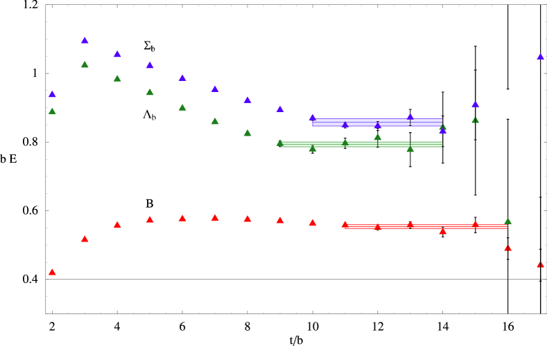
Figure 2: Effective mass ratios of the correlation functions for the $B$ (red), $\Lambda_{b}$ (green) and $\Sigma_{b}$ (violet). The shaded regions correspond to the fit range, central value and uncertainty (statistical and systematic errors are added in quadrature) for each hadron.

Hadron	fit range	$b\ {\cal E}^{(DBW2)}$	${\cal E}^{(DBW2)}$ [MeV]	$\overline{\Lambda}_{DBW2}^{(\alpha+\alpha^{2}\beta)}$ [MeV]
$B$	$11\rightarrow 15$	$0.5539(37)(50)$	$1096(18)(10)$	$649(31)(10)$
$\Lambda_{b}$	$9\rightarrow 14$	$0.7934(65)(22)$	$1570(27)(04)$	$1123(36)(04)$
$\Sigma_{b}$	$10\rightarrow 14$	$0.8575(74)(74)$	$1697(29)(15)$	$1250(38)(15)$

Table 2: The spectrum of hadrons comprised of one static color ${\bf 3}$ source and light (anti-)quarks, for a light quark mass giving the light hadron spectrum shown in Table. 1. ${\cal E}^{(DBW2)}$ is the mass of the hadron determined in the lattice calculation. $\overline{\Lambda}^{(\alpha+\alpha^{2}\beta)}_{DBW2}={\cal E}^{(DBW2)}-\delta m^{(\alpha+\alpha^{2}\beta)}_{DBW2}$ is the BLM-improved determination of the energy of the ldof. The first uncertainty is statistical and the second uncertainty is systematic.

	Hadrons	$b\,{\cal E}=b\,\delta\overline{\Lambda}$	$\delta\overline{\Lambda}$ [MeV]
	$\Lambda_{b}-B$	$0.2395(75)(72)$	$474(15)(14)$
	$\Sigma_{b}-B$	$0.304(08)(12)$	$601(16)(24)$
	$\Sigma_{b}-\Lambda_{b}$	$0.0641(98)(96)$	$126(19)(19)$

Table 3: The mass differences between the hadrons comprised of one static color ${\bf 3}$ source and light (anti-)quarks. The residual mass of the static source cancels in the differences, leaving the differences between the energy of the light degrees of freedom, denoted by $\delta\overline{\Lambda}$. The first uncertainty is statistical and the second is systematic.

IV Exotic Baryons

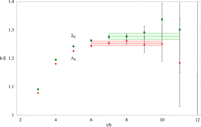
Figure 3: The effective mass plots for the exotic hadrons, $\Lambda_{\overline{\bf 6}}$ and $\Sigma_{\overline{\bf 6}}$.

Hadron	fit range	$b\ {\cal E}^{(DBW2)}$	${\cal E}^{(DBW2)}$ [ MeV ]	$\overline{\Lambda}_{\overline{\bf 6};DBW2}^{(\alpha+\alpha^{2}\beta)}$ [ MeV ]
$\Lambda_{\overline{\bf 6}}$	$6\rightarrow 10$	$1.253(08)(02)$	$2480(16)(04)$	$1364(64)(04))$
$\Sigma_{\overline{\bf 6}}$	$7\rightarrow 11$	$1.278(10)(05)$	$2529(20)(10)$	$1413(65)(10)$
		$b\,\delta{\cal E}^{(DBW2)}$	$\delta\overline{\Lambda}$
$\Sigma_{\overline{\bf 6}}-\Lambda_{\overline{\bf 6}}$	–	$0.025(13)(05)$	$49(25)(11)$

Table 4: The spectrum of exotic baryons comprised of a static color ${\bf 6}$ source and light anti-quarks, for a light quark mass giving the light hadron spectrum shown in Table. 1. ${\cal E}^{(DBW2)}$ is the mass of the hadron determined in the lattice calculation. Using the BLM-improved one-loop lattice perturbation theory calculation of the residual mass, as discussed in the text, we present results for $\overline{\Lambda}^{(\alpha+\alpha^{2}\beta)}_{\overline{\bf 6};DBW2}={\cal E}^{(DBW2)}-\delta m^{(\alpha+\alpha^{2}\beta)}_{{\bf 6};DBW2}$, where the residual mass term is evaluated at the scale $q^{*(DBW2)}$ given in the text. The difference between the masses of the exotic states is given in the last line.

As a by-product of computing the potential between two $B$-mesons, we have computed the masses of baryons formed from a static-source transforming in the ${\bf 6}$ of color and two light anti-quarks with $(I,s_{l})=(0,1)$, which we denote as $\Lambda_{\overline{\bf 6}}$, or $(I,s_{l})=(1,0)$, which we denote as $\Sigma_{\overline{\bf 6}}$. These are calculated by putting two static sources, each in the ${\bf 3}$ of color at the same point in space, and requiring the light anti-quarks to have the appropriate values of $(I,s_{l})$. As the spin of the ldof decouples from the static source(s) and is a good quantum number, the ldof form a color $\overline{\bf 6}$. While the Casimir of the $\overline{\bf 3}$ representation is $C(\overline{\bf 3})=4/3$, it is $C({\bf 6})=10/3$ for the ${\bf 6}$ representation, and the residual mass that must be subtracted from the energy calculated on the lattice is $\delta m_{{\bf 6};{\rm DBW2}}^{(\alpha+\alpha^{2}\beta)}=1116\pm 62~{}{\rm MeV}$. The effective mass plots for these hadrons are shown in Fig. 3 and the energies of the ldof are shown in Table 4. These states are considerably more massive than the non-exotic hadrons and achieve plateaus at earlier times. As such exotic baryons have not been observed and heavy quarks transforming in the ${\bf 6}$ (or other higher representations) of color are not required in nature (see Refs. Wilczek:1976qi ; Karl:1976jk ; Marciano:1980zf for a number of proposals) and are not expected to be found, we do not dwell on these results further.

V B-meson Potentials

In the heavy-quark limit, the separation between the two $B$-mesons is a good quantum number and the potential, $V({\bf r})$, is simply defined by the difference between the energy of the two $B$-mesons separated by a displacement vector ${\bf r}$ (defined by the separation of the static ${\bf 3}$ color sources) and the energy of two infinitely separated $B$-mesons,

$$V_{I,s_{l}}({\bf r}) = E_{I,s_{l}}({\bf r})\ -\ 2M_{B}\ =\ \overline{\Lambda}_{I,s_{l}}({\bf r})\ -\ 2\overline{\Lambda}_{{1\over 2},{1\over 2}}\ \ \ ,$$ (19)

where the isospin and spin of the ldof can take the values $I=0,1$ and $s_{l}=0,1$. Contributing to both of these energies are the interactions between the ldof, the interactions between the ldof and the static sources, and the interactions between the static sources. As $|{\bf r}|\rightarrow\infty$, each of the contributions factorize, leaving the contribution from two non-interacting $B$-mesons, and therefore a vanishing potential.

The lattice calculation is a straightforward extension of the calculation of $\overline{\Lambda}$ for the heavy hadrons. The energy, ${\cal E}_{I,s_{l}}^{BB}({\bf r})$, of two $B$-mesons composed of static sources and light-quarks, placed on the lattice with relative displacement ${\bf r}$, is computed using the correlators in Section II. The potential computed on the lattice then becomes

$$V_{I,s_{l}}^{\rm latt}({\bf r}) = {\cal E}_{I,s_{l}}^{BB}({\bf r})\ -\ 2\ {\cal E}_{{1\over 2},{1\over 2}}\ \ \ ,$$ (20)

where

$${\cal E}_{I,s_{l}}^{BB}({\bf r})=\overline{\Lambda}_{I,s_{l}}({\bf r})-\delta{\cal V}_{R}({\bf r})+2\delta m\ \ \ ,$$ (21)

(the subscript $R$ labels the color representation of the heavy quark system dictated by the light quantum numbers $I$ and $s_{l}$). The residual masses of the static sources induced by interactions with the gauge fields cancel in $V_{I,s_{l}}^{\rm latt}({\bf r})$. However, a perturbative subtraction corresponding to the differences in interactions between the static sources in the continuum and on the lattice, (which at leading order in the strong coupling arises from one gluon exchange (OGE)) $\delta{\cal V}_{R}({\bf r})={\cal V}_{\rm OGE}^{\rm cont}-{\cal V}_{\rm OGE}^{\rm latt}$ remains. Therefore, the energies measured in the lattice calculation, and the potential between two $B$-mesons in the continuum are related by

$$V_{I,s_{l}}({\bf r}) = {\cal E}_{I,s_{l}}^{BB}({\bf r})\ -\ 2{\cal E}_{{1\over 2},{1\over 2}}\ +\ \delta{\cal V}_{R}({\bf r})\ \ \ .$$ (22)

In the cases where the spin of the ldof is $s_{l}=1$, the potential receives contributions from both a central component and a tensor component,

$$V^{(S=1)}({\bf r}) = V_{C}(r)\ +\ \hat{S}_{12}\ V_{T}(r)\,,$$ (23)

where

$$\hat{S}_{12} = {3\over 2}\left(\hat{S}_{+}(\hat{r}_{x}-i\hat{r}_{y})+\hat{S}_{-}(\hat{r}_{x}+i\hat{r}_{y})+2\hat{S}_{z}\hat{r}_{z}\right)^{2}\ -\ 2\hat{S}^{2}\ \ \ ,$$ (24)

$\hat{S}_{i}$ are the spin operators, and $\hat{\bf r}$ is the unit vector in the direction of the displacement. It follows that the central and tensor potentials can be determined from the potential at $x$ and $z$ displacements,

$$V_{C}^{(S=1)}(r) = {1\over 3}\ \left(\ V^{(S=1)}(r\ \hat{\bf e}_{z})\ +\ 2V^{(S=1)}(r\ \hat{\bf e}_{x})\ \right)$$

$$V_{T}^{(S=1)}(r) = {1\over 3}\ \left(\ V^{(S=1)}(r\ \hat{\bf e}_{z})\ -\ V^{(S=1)}(r\ \hat{\bf e}_{x})\ \right)\ \ \ ,$$ (25)

where $\hat{\bf e}_{j}$ is the unit-vector in the “$j$” direction.

V.1 Lattice Spacing Effects in a Finite-Volume

The potential measured in the lattice calculation will differ from that at infinite-volume due to the presence of image $B$-mesons resulting from the periodic boundary conditions in the spatial directions of the lattice. Therefore, the single particle energies that are extracted correspond to the energy of single particle that is interacting with its images, located at $|{\bf r}|>L$. In the case of the energy of two particles interacting in a periodic cubic volume, the potential energy, $V^{(L)}({\bf r})$, measured includes the sum over the contributions from the images

$$V^{(L)}({\bf r}) = V({\bf r})\ +\ \sum_{{\bf n}\neq{\bf 0}}\ V({\bf r}+{\bf n}L)\,.$$ (26)

When the displacement between the mesons is $|{\bf r}|>L/2$ the interaction with the nearest image is more important than the interaction within the volume. Consequently, we have only computed the potential for $|{\bf r}|\leq 8$ lattice spacings on $16^{3}\times 32$ lattices. After taking the continuum limit of the lattice calculation, the finite-volume effects due to the images must be removed to recover the infinite-volume continuum limit potential, $V({\bf r})$. This is discussed below.

The finite lattice spacing, $b$, eliminates ultraviolet modes on the lattice leaving $|{\bf q}|<\pi/b$, and hence the strong Coulomb potential that exists between two static-sources due to OGE is significantly modified for $|{\bf r}|$ less than a few $b$. In the heavy-quark limit, the OGE potential is spin-independent but does depend upon the color representation of the combined heavy quark system.

The potential between two static color ${\bf 3}$ sources combined into a color $\overline{\bf 3}$, at a finite lattice spacing, $b$, and in a finite-volume becomes

$${\cal V}_{\overline{\bf 3};LO}^{\rm latt}({\bf r})\ =\ -{\overline{\alpha}(\mu)\over 3\pi^{2}b}\ \int_{-{\pi}}^{\pi}\ d\tilde{q}_{x}\ \int_{-{\pi}}^{\pi}\ d\tilde{q}_{y}\ \int_{-{\pi}}^{\pi}\ d\tilde{q}_{z}\ G_{00}(\hat{\bf q})\ e^{i\tilde{\bf q}\cdot\tilde{\bf r}}$$

$$\rightarrow-{\overline{\alpha}(\mu)\over 3\pi^{2}b}\ \left({2\pi\over\tilde{L}}\right)^{3}\ \sum_{{\bf n}}^{|n_{i}|\leq{\tilde{L}\over 2}}\ e^{i2\pi{\bf n}\cdot\tilde{\bf r}/\tilde{L}}\ G_{00}\left(2\sin\left({\pi n_{x}\over\tilde{L}}\right),2\sin\left({\pi n_{y}\over\tilde{L}}\right),2\sin\left({\pi n_{z}\over\tilde{L}}\right),0\right)\ ,$$ (27)

where $\tilde{L}=L/b$ is the spatial extent of the lattice in lattice units, and ${\bf\tilde{r}}={\bf r}/b$ is the displacement between the static sources in lattice units. The summation in Eq. (27) is over all $-\tilde{L}/2<n_{x},n_{y},n_{z}<\tilde{L}/2$. This finite-volume expression has an infrared divergence due to the ${\bf n}={\bf 0}$ mode, however, the difference between the finite-volume OGE potentials at finite lattice spacing and in the continuum is of the form

$$\delta{\cal V}_{\overline{\bf 3};LO}^{(L)}({\bf r}) = -{\overline{\alpha}(\mu)\over 3\pi^{2}b}\ \left({2\pi\over\tilde{L}}\right)^{3}\ \left[\ \left({\tilde{L}\over 2\pi}\right)^{2}\sum_{\bf n}^{\infty}\ \frac{e^{i2\pi{\bf n}\cdot\tilde{\bf r}/\tilde{L}}\ }{|{\bf n}|^{2}}-\sum_{{\bf n}}^{|n_{i}|\leq{\tilde{L}\over 2}}\ e^{i2\pi{\bf n}\cdot\tilde{\bf r}/\tilde{L}}\ G_{00}\left(\hat{n}_{x},\hat{n}_{y},\hat{n}_{z},0\right)\ \right]\ ,$$

where $\hat{n}_{i}=2\sin\left(\pi n_{i}/\tilde{L}\right)$, and is well-behaved in the infrared. Spurious contributions from ill-defined low-momentum gluon modes included in the above sums cancel to a large extent with residual effects at most of ${\cal O}(b^{2})$. Further discussion of this issue and the numerical evaluation of $\delta{\cal V}_{\overline{\bf 3};LO}^{(L)}({\bf r})$ can be found in Appendix B.

The BLM procedure is again used to set the scale of the correction factor, leading to

$$\delta{\cal V}_{\overline{\bf 3};NLO}^{(L)}({\bf r}) = -{\overline{\alpha}(\mu)\over 3\pi^{2}b}\ \left({2\pi\over\tilde{L}}\right)^{3}\ \left[\left({\tilde{L}\over 2\pi}\right)^{2}\sum_{\bf n}^{\infty}\ \ {e^{i2\pi{\bf n}\cdot\tilde{\bf r}/\tilde{L}}\over|{\bf n}|^{2}}\left(1\ -\ {\overline{\alpha}(\mu)\beta\over 4\pi}\log\left({4\pi^{2}\left(|{\bf n}|^{2}\right)\over\mu^{2}L^{2}}\right)\ \right)\right.$$ (29)

$$\left.\ -\ \sum_{{\bf n}}^{|n_{i}|\leq{\tilde{L}\over 2}}\ e^{i2\pi{\bf n}\cdot\tilde{\bf r}/\tilde{L}}\ G_{00}\left(\hat{n}_{x},\hat{n}_{y},\hat{n}_{z},0\right)\left(1\ -\ {\overline{\alpha}(\mu)\beta\over 4\pi}\log\left({|\hat{\bf n}|^{2}\over\mu^{2}b^{2}}\right)\right)\ \right]$$

$$= -{\overline{\alpha}(\mu)\over r}\left[\ {\cal A}\left(\tilde{\bf r},\tilde{L}\right)\ -\ {\overline{\alpha}(\mu)\beta\over 4\pi}{\cal B}\left(\tilde{\bf r},\tilde{L},\mu\right)\ \right]$$

$$= -{\overline{\alpha}(q^{*}(\tilde{\bf r},\tilde{L}))\over r}\ {\cal A}\left(\tilde{\bf r},\tilde{L}\right)\ +\ ...\ .$$

The coefficient functions ${\cal A}(\tilde{\bf r},\tilde{L})$ and ${\cal B}(\tilde{\bf r},\tilde{L},\mu)$ evaluated on DBW2 lattices, using the techniques in Appendix B, are given in Table. 5 at the required separations. The resulting BLM-scale and potential shifts are given in Table. 6 (results for the color ${\bf 6}$ OGE potential are related by $\delta{\cal V}_{{\bf 6};(N)LO}^{(L)}({\bf r})=-1/2\,\delta{\cal V}_{\overline{\bf 3};(N)LO}^{(L)}({\bf r})$). The correction factors, $\delta{\cal V}_{\overline{\bf 3};LO}^{(L)}({\bf r})$ and $\delta{\cal V}_{{\bf 6};LO}^{(L)}({\bf r})$, should be added to the lattice measurements of ${\cal E}_{I,s_{l}}-2{\cal E}_{\frac{1}{2},\frac{1}{2}}$ to give the potential. At relative displacements that are large compared with the lattice spacing, this correction factor scales as $b^{2}/|{\bf r}|^{3}$, as expected. However, there are still ${\cal O}(b)$ lattice artifacts from the discretisation of the light quark sector. These can only be eliminated using data at different lattice spacings or using a light-quark action that is ${\cal O}(b)$-improved.

$\tilde{\bf r}$	${\cal A}(\tilde{\bf r},16)$	${\cal B}(\tilde{\bf r},16,b^{-1})$	${\cal A}(\tilde{\bf r},\infty)$	${\cal B}(\tilde{\bf r},\infty,b^{-1})$
$(1,0,0)$	$+0.2656$	$-0.04261$	0.2654	-0.0938
$(1,1,0)$	$+0.2011$	$-0.1791$	0.2102	-0.2236
$(2,0,0)$	$+0.1203$	$-0.2352$	0.1629	-0.2451
$(2,1,0)$	$+0.1144$	$-0.2130$	0.1370	-0.2750
$(3,0,0)$	$+0.1206$	$-0.0750$	0.1083	-0.2357
$(4,0,0)$	$-0.0176$	$-0.1975$	0.0665	-0.2048
$(5,0,0)$	$+0.0592$	$+0.0874$	0.0370	-0.1653
$(6,0,0)$	$-0.1055$	$-0.1359$	0.0176	-0.1261
$(7,0,0)$	$+0.0409$	$+0.2310$	0.0054	-0.0921
$(8,0,0)$	$-0.1593$	$-0.1247$	0.0020	-0.0647

Table 5: The functions ${\cal A}(\tilde{\bf r},\tilde{L})$ and ${\cal B}(\tilde{\bf r},\tilde{L},\mu)$ that contribute to the difference between the finite-lattice spacing and continuum OGE potentials at finite-volume.

$\tilde{\bf r}$	$b\,q^{*}(\tilde{\bf r},16)$	$b\ \delta{\cal V}_{\overline{\bf 3};LO}^{(L)}({\bf r})$	$b\ \delta{\cal V}_{\overline{\bf 3};NLO}^{(L)}({\bf r})$	$\delta{\cal V}_{\overline{\bf 3};NLO}^{(L)}({\bf r})$ [ MeV ]
$(1,0,0)$	$0.9229$	$-0.0794(40)$	$-0.0828(41)$	$-163.8(8.6)$
$(1,1,0)$	$0.6406$	$-0.0425(21)$	$-0.0524(26)$	$-103.7(5.4)$
$(2,0,0)$	$0.3762$	$-0.01798(90)$	$-0.0272(14)$	$-53.8(2.8)$
$(2,1,0)$	$0.3941$	$-0.01529(77)$	$-0.0227(11)$	$-45.0(2.4)$
$(3,0,0)$	$0.7327$	$-0.01202(60)$	$-0.01398(70)$	$-27.7(1.4)$
$(4,0,0)$	$269.6$	$+0.001319(66)$	$-0.00254(13)$	$-5.04(26)$
$(5,0,0)$	$2.092$	$-0.00354(18)$	$-0.00217(10)$	$-4.30(23)$
$(6,0,0)$	$1.904$	$+0.00525(26)$	$+0.00348(17)$	$+6.90(36)$
$(7,0,0)$	$16.87$	$-0.001747(87)$	$+0.000836(42)$	$+1.654(87)$
$(8,0,0)$	$1.479$	$+0.00595(30)$	$+0.00473(24)$	$+9.37(49)$

Table 6: Corrections to the potential between two static color ${\bf 3}$ sources combined into the $\overline{\bf 3}$ representation, displaced by $\tilde{\bf r}$ computed on $16^{3}\times 32$ DBW2 lattices with a lattice spacing of $b=0.0997\pm 0.0015~{}{\rm fm}$. The quoted uncertainty is due to the uncertainty in $\alpha_{s}(2~{}{\rm GeV})$, and that of the lattice spacing. The NLO result does not use the BLM scale, $q^{*}$, but the sum of the LO and NLO contributions.

V.2 The Lattice and Continuum Finite-Volume Potentials

Using the techniques described in Sec. II we have computed the correlation functions corresponding to the energy differences of Eq. (20). Correlated and uncorrelated single exponential fits to the correlation functions are performed to determine the energy of the two B-mesons, and the Jackknife method is used to determine the uncertainty. Further, Jackknife is used to determine the correlated difference in energy between the two $B$-mesons, and twice the single $B$-meson mass.

The effective mass plots for the correlators defining the central potentials at $|\tilde{\bf r}|=0,1,2,3,4,5,6,7,8$ are shown in Fig. 4 and those for the potentials at displacements of $\tilde{\bf r}=(1,1,0)$ and $(2,1,0)$ are shown in Fig. 5. It is not possible to further decompose these latter potentials into the central and tensor components, without additional information. However, given that the tensor potentials at all the other displacements are found to be very small, it is not unreasonable to assume that they are also small for these displacements, and therefore we can assume that they provide a good determination of the central potentials alone. For a number of combinations of $I$, $s_{l}$ and $\tilde{\bf r}$, it was not possible to extract a signal and these points are omitted in the effective mass plots and tables below.

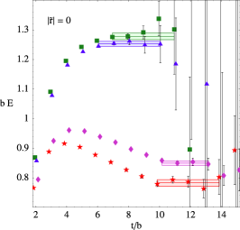
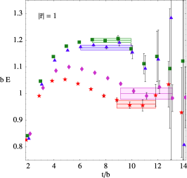
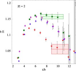
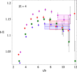
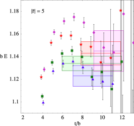
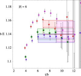
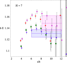
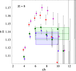
Figure 4: The effective mass plots for the central potentials at $|\tilde{\bf r}|=0,1,2,3,4,5,6,7,8$ for each spin-isospin channel. Red stars correspond to $(I,s_{l})=(0,0)$, green squares to $(I,s_{l})=(1,0)$, blue triangles to $(I,s_{l})=(0,1)$ and magenta diamonds to $(I,s_{l})=(1,1)$. Extracted masses and uncertainties are shown as the shaded regions in channels where a signal can be extracted, and are given in Tables 7-10.

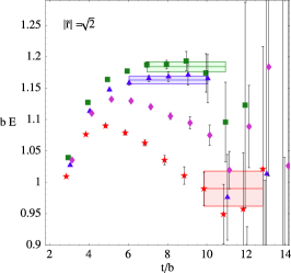
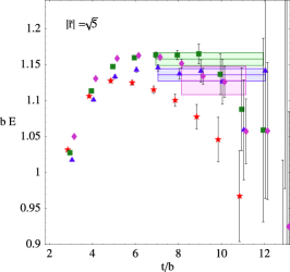
Figure 5: The effective mass plots for the potentials at displacements $\tilde{\bf r}=(1,1,0)$ and $(2,1,0)$ which are linear combinations of the central and tensor potentials. Red stars correspond to $(I,s_{l})=(0,0)$, green squares to $(I,s_{l})=(1,0)$, blue triangles to $(I,s_{l})=(0,1)$ and magenta diamonds to $(I,s_{l})=(1,1)$. Extracted masses and uncertainties are shown as the shaded regions in channels where a signal can be extracted, and are given in Tables 7-10.

$\tilde{r}$	$b\ {\cal E}^{BB}_{00}(\tilde{r})$	$b\ V^{{\rm latt}(L)}_{I=S=0}(\tilde{r})$	$b\ V^{(L)}_{I=S=0}(\tilde{r})$	$V^{(L)}_{I=S=0}(\tilde{r})$ [MeV]
0	$0.783(11)(02)$	$-0.325(13)(10)$	$-\infty$	$-\infty$
1	$0.960(12)(08)$	$-0.148(14)(13)$	$-0.231(15)(13)$	$-456(30)(25)$
$\sqrt{2}$	$0.990(27)(07)$	$-0.118(28)(12)$	$-0.170(28)(12)$	$-337(56)(24)$
2	$1.056(13)(08)$	$-0.052(15)(13)$	$-0.079(15)(13)$	$-156(30)(25)$
$\sqrt{5}$	—	—	—	—
3	$1.097(20)(15)$	$-0.011(21)(18)$	$-0.025(21)(18)$	$-49(42)(36)$
4	$1.132(12)(06)$	$0.024(14)(12)$	$0.022(14)(11)$	$43(28)(23)$
5	$1.143(09)(05)$	$0.035(12)(11)$	$0.033(12)(11)$	$65(23)(22)$
6	$1.150(09)(05)$	$0.042(12)(11)$	$0.046(12)(11)$	$90(23)(22)$
7	—	—	—	—
8	—	—	—	—

Table 7: The extracted lattice and continuum potentials in the $I=S=0$ channel. The first uncertainty is statistical, while the second is systematic.

$\tilde{r}$	$b\ {\cal E}^{BB}_{10}(\tilde{r})$	$b\ V^{{\rm latt}(L)}_{I=1,S=0}(\tilde{r})$	$b\ V^{(L)}_{I=1,S=0}(\tilde{r})$	$V^{(L)}_{I=1,S=0}(\tilde{r})$ [MeV]
0	$1.278(10)(05)$	$+0.170(12)(11)$	$+\infty$	$+\infty$
1	$1.199(07)(03)$	$+0.091(10)(10)$	$+0.133(10)(10)$	$+262(21)(21)$
$\sqrt{2}$	$1.184(08)(01)$	$+0.076(11)(10)$	$+0.102(11)(10)$	$+203(22)(20)$
2	$1.158(07)(02)$	$+0.050(10)(10)$	$+0.064(10)(10)$	$+126(20)(20)$
$\sqrt{5}$	$1.158(09)(01)$	$+0.050(12)(10)$	$+0.062(12)(10)$	$+122(23)(20)$
3	$1.142(06)(06)$	$+0.034(10)(12)$	$+0.041(10)(12)$	$+82(19)(23)$
4	—	—	—	—
5	$1.134(05)(04)$	$+0.026(09)(11)$	$+0.027(09)(11)$	$+54(18)(21)$
6	$1.140(07)(04)$	$+0.032(10)(11)$	$+0.030(10)(11)$	$+60(20)(21)$
7	—	—	—	—
8	$1.138(07)(03)$	$+0.030(10)(10)$	+$0.028(10)(10)$	$+55(20)(21)$

Table 8: The extracted lattice and continuum potentials in the $I=1,S=0$ channel. The first uncertainty is statistical, while the second is systematic.

$\tilde{r}$	$b\ {\cal E}^{BB}_{11}(\tilde{r})$	$b\ V^{{\rm latt}(L)}_{I=S=1}(\tilde{r})$	$b\ V^{(L)}_{I=S=1}(\tilde{r})$	$V^{(L)}_{I=S=1}(\tilde{r})$ [MeV]
0	$0.850(06)(04)$	$-0.258(09)(11)$	$-\infty$	$-\infty$
1	$1.000(12)(18)$	$-0.108(14)(21)$	$-0.191(15)(21)$	$-377(30)(41)$
$\sqrt{2}^{*}$	—	—	—	—
2	—	—	—	—
$\sqrt{5}^{*}$	$1.128(18)(08)$	$+0.020(20)(13)$	$-0.003(20)(13)$	$-05(38)(25)$
3	$1.140(10)(10)$	$+0.032(12)(14)$	$+0.018(12)(14)$	$+36(25)(28)$
4	$1.150(10)(10)$	$+0.042(12)(14)$	$+0.040(12)(14)$	$+78(25)(28)$
5	$1.145(10)(15)$	$+0.037(12)(18)$	$+0.035(12)(18)$	$+69(25)(36)$
6	$1.1544(12)(09)$	$+0.036(14)(13)$	$+0.040(14)(13)$	$+79(28)(27)$
7	$1.149(10)(09)$	$0.041(12)(13)$	$0.042(12)(13)$	$+83(25)(27)$
8	—	—	—	—

Table 9: The extracted lattice and continuum central potentials in the $I=S=1$ channel. The first uncertainty is statistical, while the second is systematic. The asterisks attached to the $r=\sqrt{2}$ and $\sqrt{5}$ potentials indicate that these are the sum of the central and tensor contributions.

$\tilde{r}$	$b\ {\cal E}^{BB}_{01}(\tilde{r})$	$b\ V^{{\rm latt}(L)}_{I=0,S=1}(\tilde{r})$	$b\ V^{(L)}_{I=0,S=1}(\tilde{r})$	$V^{(L)}_{I=0,S=1}(\tilde{r})$ [MeV]
0	$1.253(08)(02)$	$+0.145(11)(10)$	$+\infty$	$+\infty$
1	$1.172(07)(05)$	$+0.064(10)(11)$	$+0.106(10)(11)$	$+209(21)(22)$
$\sqrt{2}^{*}$	$1.163(06)(01)$	$+0.055(10)(10)$	$0.081(10)(10)$	$+161(19)(20)$
2	—	—	—	—
$\sqrt{5}^{*}$	$1.136(08)(03)$	$+0.028(11)(10)$	$+0.040(11)(10)$	$+78(22)(21)$
3	—	—	—	—
4	$1.128(07)(04)$	$+0.020(10)(11)$	$+0.021(10)(11)$	$+42(20)(21)$
5	$1.123(07)(06)$	$+0.015(10)(11)$	$+0.016(10)(12)$	$+32(20)(23)$
6	$1.134(06)(02)$	$+0.026(10)(10)$	$+0.024(10)(10)$	$+48(19)(20)$
7	$1.149(10)(09)$	$0.041(12)(13)$	$0.042(12)(13)$	$+83(25)(27)$
8	$1.131(06)(03)$	$0.023(10)(10)$	$0.021(10)(10)$	$+41(19)(21)$

Table 10: The extracted lattice and continuum central potentials in the $I=0,S=1$ channel. The first uncertainty is statistical, while the second is systematic. The asterisks attached to the $r=\sqrt{2}$ and $\sqrt{5}$ potentials indicate that these are the sum of the central and tensor contributions.

After applying the perturbative one-loop matching discussed above, we determine the various finite-volume potentials. The central potentials extracted from the lattice calculation in each of the spin-isospin channels are given in Tables 7-10. The lattice central potentials, $V^{{\rm latt}(L)}_{I,s_{l}}$, are shown in Fig. 6, and the central potentials with the leading order finite-lattice spacing correction included (as discussed above), $V^{(L)}_{I,s_{l}}$, are shown in Fig. 7. In each channel there is a clean signal for the central potentials, with two or more of the displacements having potentials that are clearly non-zero. For the $s_{l}=1$ channels the tensor potentials are found to be consistent with zero and are smaller than $V_{T}\sim 40~{}{\rm MeV}$ in both cases for the entire range of displacements (the tensor potentials were also found to small and poorly determined in Ref. Michael:1999nq ). At large distances, this is not consistent with our expectations from the NN system at the physical value of $m_{\pi}$, but may result from the relevant $B^{(\ast)}B^{(\ast)}M$ couplings ($M$ represents the various mesons) being small or giving rise to cancellations, or from the unphysically large pion mass. Further studies of this issue are warranted. The measurements at $\tilde{\bf r}=0$ contain no information about the continuum potentials, which diverge as $\sim\overline{\alpha}(r^{-1})/r$. As discussed in Sections III and IV, the lattice energies measured for coincident $B$-mesons, in fact, determine the energies of the $\Lambda_{b}$ and $\Sigma_{b}$ and their exotic partners.

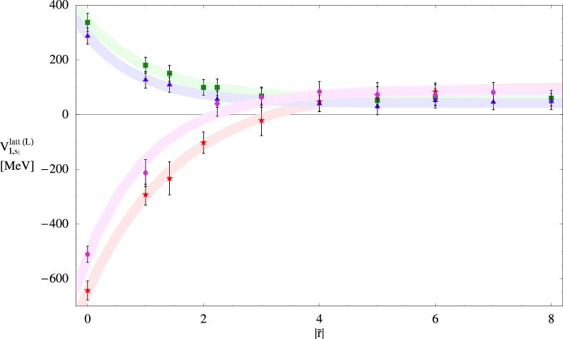
Figure 6: The finite-volume and finite-lattice spacing central potentials, $V^{{\rm latt}(L)}_{I,s_{l}}$, extracted from the lattice calculation. The shaded regions are simple fits to guide the eye. Red stars, green squares, blue triangles and magenta diamonds correspond to $(I,s_{l})\ =\ (0,0),\,(1,0),\,(0,1),\,(1,1)$ respectively.

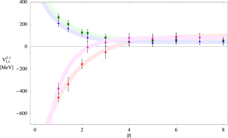
Figure 7: The finite-volume central potentials extracted from the lattice calculation including the leading lattice correction to OGE, $V^{(L)}_{I,s_{l}}$. The shaded regions are simple fits to guide the eye. Red stars, green squares, blue triangles and magenta diamonds correspond to $(I,s_{l})\ =\ (0,0),\,(1,0),\,(0,1),\,(1,1)$ respectively.

V.3 Potentials with $t$-Channel Quantum Numbers

Up until this point we have classified the potentials between the B-mesons in terms of the $s$-channel quantum numbers, the total isospin and spin of the ldof. These potentials are extracted from the energies calculated on the lattice by subtracting twice the $B$-meson mass. The statistical and systematic uncertainty in determining the B-meson mass propagates through to all four central potentials, leading to larger uncertainties in the potential than from the calculation of the energy of the two $B$-mesons alone. Motivated by the success of traditional nuclear physics phenomenological potentials constructed from the exchange of mesons in the $t$-channel, we have formed linear combinations of the $s$-channel potentials to give potentials with well-defined spin and isospin quantum numbers that can be identified with the exchange of one or more hadrons. The central potential can be decomposed as

$$V_{I,s_{l}}(|{\bf r}|)=V_{1}(|{\bf r}|)\ +\ \sigma_{1}\cdot\sigma_{2}\ V_{\sigma}(|{\bf r}|)\ +\ \sigma_{1}\cdot\sigma_{2}\,\tau_{1}\cdot\tau_{2}\,V_{\sigma\tau}(|{\bf r}|)\ +\ \tau_{1}\cdot\tau_{2}\ V_{\tau}(|{\bf r}|)\ \ ,$$ (30)

where it is straightforward to show that, in terms of the s-channel central potentials,

$$V_{1} = \frac{1}{16}\left(V_{0,0}+3V_{0,1}+3V_{1,0}+9V_{1,1}\right)\,,$$

$$V_{{\sigma}} = \frac{1}{16}\left(-V_{0,0}+V_{0,1}-3V_{1,0}+3V_{1,1}\right)\,,$$

$$V_{{\sigma\tau}} = {1\over 16}\left(V_{0,0}-V_{0,1}-V_{1,0}+V_{1,1}\ \right)\,,$$

$$V_{{\tau}} = \frac{1}{16}\left(-V_{0,0}-3V_{0,1}+V_{1,0}+3V_{1,1}\right)\,.$$ (31)

An important point to observe is that the three potentials, $V_{{\sigma}}$, $V_{{\sigma\tau}}$ and $V_{{\tau}}$ can be extracted from the lattice calculation without reference to the $B$-meson mass. This is not true for $V_{1}$. It was pointed out in Ref. Beane:2002nu that the $\eta^{\prime}$ double-pole that is present in quenched calculations will dominate the interactions between nucleons and $B$-mesons at long-distances. However, we see that this can only contribute to $V_{{\sigma}}$, and not to the other three potentials. Further, the exchange of a single $\pi$ will contribute only to the $V_{{\sigma\tau}}$ potential. Therefore, the potential $V_{{\tau}}$ does not receive contributions from hairpins nor from $\pi$-exchange, and does not depend upon the $B$-meson mass extraction from the lattice calculation. It is expected to be clean, and determined by short-range and medium range interactions.

$\tilde{r}$	$b\ V^{{\rm latt}(L)}_{\sigma}(\tilde{r})$	$b\ V^{(L)}_{\sigma}(\tilde{r})$	$V^{(L)}_{\sigma}(\tilde{r})$ [MeV]
0	-0.050(17)(06)	$-\infty$	$-\infty$
1	-0.0174(33)(08)	-0.0337(34)(08)	-66.8(6.8)(1.7)
$\sqrt{2}^{*}$	-0.0081(25)(02)	-0.0178(25)(02)	-35.1(5.1)(0.3)
2	—	—	—
$\sqrt{5}^{*}$	-0.0016(25)(09)	-0.0049(25)(09)	-9.7(5.0)(1.8)
3	+0.0035(13)(00)	+0.0008(12)(00)	+1.6(2.6)(0.1)
4	+0.0048(13)(08)	+0.0035(13)(08)	+6.9(2.6)(1.5)
5	+0.0054(12)(05)	+0.0044(12)(05)	+8.8(2.4)(1.0)
6	—	—	—
7	+0.0054(18)(02)	+0.0054(18)(02)	+10.7(3.6)(0.3)
8	+0.0047(16)(03)	+0.0053(16)(03)	+10.5(3.1)(0.6)

Table 11: The extracted lattice and continuum central potential $V^{(L)}_{\sigma}$, defined in Eq. (V.3). The first uncertainty is statistical, while the second is systematic. The asterisks attached to the $r=\sqrt{2}$ and $\sqrt{5}$ potentials indicate that these are the sum of the central and tensor contributions.

$\tilde{r}$	$b\ V^{{\rm latt}(L)}_{\sigma\tau}(\tilde{r})$	$b\ V^{(L)}_{\sigma\tau}(\tilde{r})$	$V^{(L)}_{\sigma\tau}(\tilde{r})$ [MeV]
0	-0.0539(56)(07)	$-\infty$	$-\infty$
1	-0.0228(24)(08)	-0.0383(25)(08)	-75.9(5.2)(1.5)
$\sqrt{2}^{*}$	-0.0158(21)(02)	-0.0256(22)(02)	-50.8(4.4)(0.3)
2	-0.0064(22)(07)	-0.0115(22)(07)	-22.7(4.3)(1.3)
$\sqrt{5}^{*}$	-0.0062(42)(05)	-0.0105(42)(05)	-20.7(8.4)(1.0)
3	-0.0003(23)(12)	-0.0029(22)(12)	-5.7(4.5)(2.3)
4	+0.00205(82)(50)	+0.00158(82)(50)	+3.1(1.6)(1.0)
5	+0.00343(09)(32)	+0.0030(09)(03)	+6.0(1.9)(0.6)
6	—	—	—
7	+0.00294(55)(07)	+0.00309(55)(07)	+6.1(1.1)(0.1)
8	—	—	—

Table 12: The extracted lattice and continuum central potential $V^{(L)}_{\sigma\tau}$, defined in Eq. (V.3). The first uncertainty is statistical, while the second is systematic. The asterisks attached to the $r=\sqrt{2}$ and $\sqrt{5}$ potentials indicate that these are the sum of the central and tensor contributions.

$\tilde{r}$	$b\ V^{{\rm latt}(L)}_{\tau}(\tilde{r})$	$b\ V^{(L)}_{\tau}(\tilde{r})$	$V^{(L)}_{\tau}(\tilde{r})$ [MeV]
0	-0.0390(49)(03)	$-\infty$	$-\infty$
1	-0.0136(39)(02)	-0.0292(40)(02)	-57.7(7.8)(0.4)
$\sqrt{2}^{*}$	-0.0033(31)(05)	-0.0131(31)(05)	-25.9(6.3)(1.0)
2	+0.00539(66)(02)	+0.00029(70)(02)	+0.58(1.4)(0.0)
$\sqrt{5}^{*}$	+0.00587(53)(15)	+0.00161(57)(15)	+3.2(1.2)(0.3)
3	+0.00787(71)(12)	+0.00525(73)(12)	+10.4(1.4)(0.2)
4	+0.00767(61)(22)	+0.00720(61)(22)	+14.2(1.2)(0.4)
5	+0.00664(97)(04)	+0.00623(97)(04)	+12.3(1.9)(0.1)
6	—	—	—
7	+0.00509(50)(07)	+0.00525(50)(07)	+10.4(1.0)(0.1)
8	+0.00455(62)(24)	+0.00544(62)(24)	+10.8(1.2)(0.5)

Table 13: The extracted lattice and continuum central potential $V^{(L)}_{\tau}$, defined in Eq. (V.3). The first uncertainty is statistical, while the second is systematic. The asterisks attached to the $r=\sqrt{2}$ and $\sqrt{5}$ potentials indicate that these are the sum of the central and tensor contributions.

$\tilde{r}$	$b\ V^{{\rm latt}(L)}_{1}(\tilde{r})$	$b\ V^{(L)}_{1}(\tilde{r})$	$V^{(L)}_{1}(\tilde{r})$ [MeV]
0	-0.117(16)(03)	$-\infty$	$-\infty$
1	-0.0616(96)(25)	-0.0520(96)(25)	-103(19)(04)
$\sqrt{2}^{*}$	-0.0193(74)(04)	-0.0210(74)(04)	-42(15)(0.7)
2	-0.0135(58)(18)	-0.0101(58)(18)	-20(12)(4)
$\sqrt{5}^{*}$	-0.0020(78)(10)	-0.0019(78)(10)	-4(16)(2)
3	+0.0030(43)(17)	+0.0037(43)(17)	+7.4(8.4)(3.3)
4	+0.0093(45)(10)	+0.0094(45)(10)	+16.6(8.9)(2.0)
5	+0.0069(19)(01)	+0.0064(19)(01)	+12.6(3.8)(0.1)
6	—	—	—
7	+0.0074(43)(14)	+0.0057(43)(14)	+11.2(8.4)(2.8)
8	+0.0051(29)(07)	+0.0055(29)(07)	+10.8(5.7)(1.4)

Table 14: The extracted lattice and continuum central potential $V^{(L)}_{1}$, defined in Eq. (V.3). The first uncertainty is statistical, while the second is systematic. The asterisks attached to the $r=\sqrt{2}$ and $\sqrt{5}$ potentials indicate that these are the sum of the central and tensor contributions.

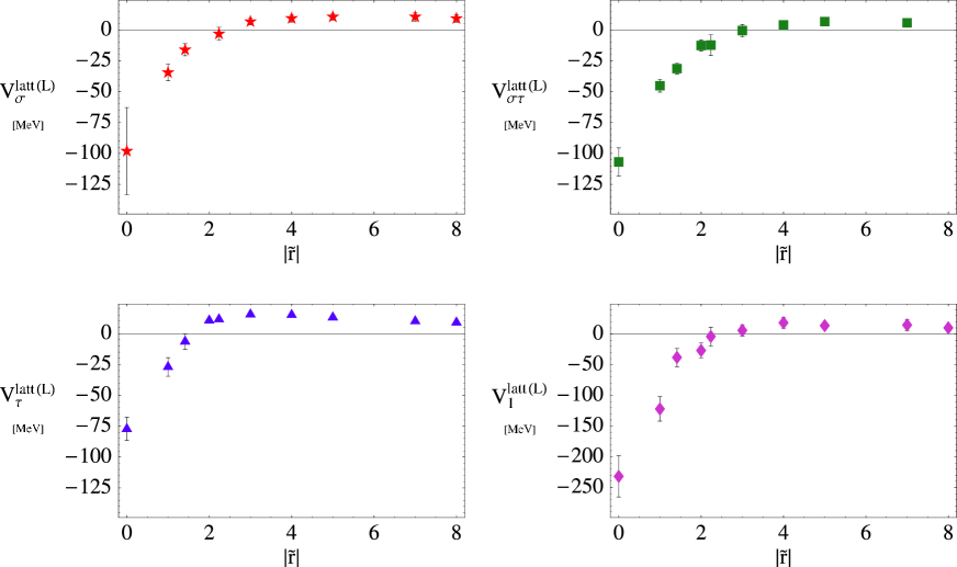
Figure 8: The central finite-volume lattice potentials $V^{{\rm latt}(L)}_{\sigma,\sigma\tau,\tau,1}$, as defined in Eq. (V.3). The statistical and systematic errors have been added in quadrature.

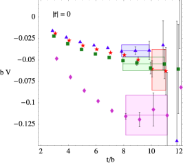
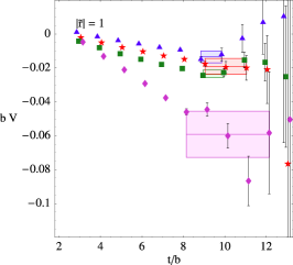
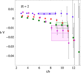
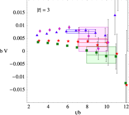
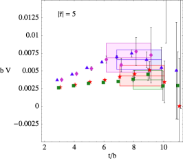
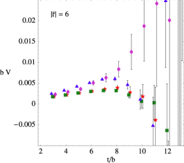
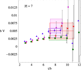
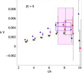
Figure 9: The effective mass plots for the central potentials at $|\tilde{\bf r}|=0,1,2,3,4,5,6,7,8$ for each $t$-channel potential. Red stars correspond to $V_{\sigma}$, green squares to $V_{\sigma\tau}$, blue triangles to $V_{\tau}$ and magenta diamonds to $V_{1}$. Extracted masses and uncertainties are shown as the shaded regions in channels where a signal can be extracted.

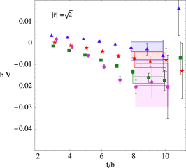
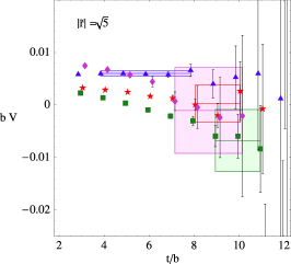
Figure 10: The effective mass plots for the potentials at displacements $\tilde{\bf r}=(1,1,0)$ and $(2,1,0)$ Red stars correspond to $V_{\sigma}$, green squares to $V_{\sigma\tau}$, blue triangles to $V_{\tau}$ and magenta diamonds to $V_{1}$. Extracted masses and uncertainties are shown as the shaded regions in channels where a signal can be extracted.

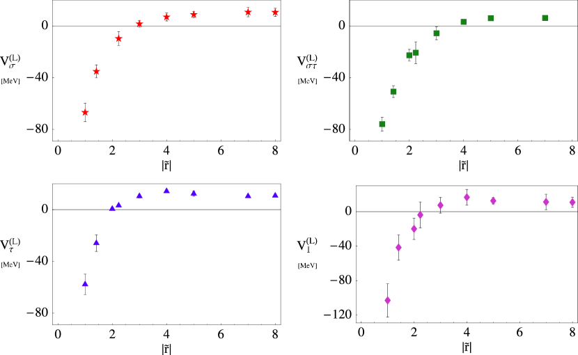
Figure 11: The central finite-volume potentials $V_{\sigma,\sigma\tau,\tau,1}$, as defined in Eq. (V.3) (the lattice potentials plus the leading lattice spacing corrections to OGE). The statistical and systematic errors have been added in quadrature.

The finite-volume potentials calculated on the lattice, $V^{{\rm latt}(L)}_{{\sigma},{\tau},{\sigma\tau},{1}}(\tilde{\bf r})$, are given in Tables 11-14, and are shown in Fig. 8. Effective mass plots for these potentials are shown in Figs. 9 and 10. The potentials corrected for the finite-lattice spacing contributions to OGE between the heavy quarks are also given in Tables 11-14, and are shown in Fig. 11. The uncertainties in these potentials are seen to be significantly smaller than those of $V_{I,s_{l}}$, in part due to the fact that the $B$-meson mass extraction, and its associated uncertainty, does not contribute. The most striking potential is $V_{\tau}$; it is clear that this potential is of shorter range than $V_{\sigma}$ and $V_{\sigma\bm{\tau}}$, due to the absence of OPE and OHE.

V.4 Extrapolation to Infinite-Volume Potentials

The final stage of analysis is to use the extracted finite-volume potentials in either the $s$- or $t$-channels to determine the infinite-volume forms. At short distances, $|{\bf r}|\lesssim\Lambda_{\chi}^{-1}$ ($|\tilde{\bf r}|\lesssim 2$ for our analysis), the infinite-volume extrapolation must be done empirically, fitting functions with the correct long-distance behavior to the results of lattice calculations in multiple volumes. In principle, this extrapolation can be performed systematically for larger $|{\bf r}|$ as effective field theory describes the potential in this regime. Here we explore how the matching to EFT can be implemented, focusing on the isovector potentials.

In QCD, the long range pieces of the infinite-volume, $t$-channel isovector potentials are expected to have the form

$$V_{\sigma\tau}^{(\infty)}({\bf r}) \stackrel{{\scriptstyle|{\bf r}|\to\infty}}{{\longrightarrow}} \ \frac{g^{2}\ m_{\pi}^{2}}{24\pi f_{\pi}^{2}}\ \frac{e^{-m_{\pi}|{\bf r}|}}{|{\bf r}|}\ +\ V_{\sigma\tau}^{(2\pi)}(|{\bf r}|)\ +\ \ldots$$ (32)

$$V_{\tau}^{(\infty)}({\bf r}) \stackrel{{\scriptstyle|{\bf r}|\to\infty}}{{\longrightarrow}} \ \frac{g_{\rho}^{2}}{4\pi}\ \frac{e^{-m_{\rho}|{\bf r}|}}{|{\bf r}|}\ +\ V_{\tau}^{(2\pi)}(|{\bf r}|)\ +\ \ldots$$ (33)

where $V_{\tau}^{(2\pi)}$ and $V_{\sigma\tau}^{(2\pi)}$ are the two pion exchange potentials defined in Ref. Kaiser:1997mw (with nucleon couplings replaced by the relevant couplings of the $B$ sector), $f_{\pi}\sim 132$ MeV, $g$ is the chiral coupling of pions to heavy mesons occurring in the heavy meson chiral perturbation theory Lagrangian Burdman:1992gh ; Wise:1992hn ; Yan:1992gz ; Booth:1994hx ; Sharpe:1995qp , and $g_{\rho}$ is a phenomenological $BB\rho$ coupling. The ellipses denote contributions suppressed at large separations.

Ideally, lattice determinations of the meson masses and potentials at long distances could be used to fit the couplings in the above equations (the two pion contributions contain additional parameters). However, a number of issues complicate this analysis. The quenched nature of our calculations introduces artefacts as in this case, the $\eta^{\prime}$ meson remains degenerate with the pions but has a modified propagator Bernard:1992mk ; Sharpe:1992ft ,

$$G_{\eta^{\prime}}(q^{2}) = \frac{i}{q^{2}-m_{\pi}^{2}+i\epsilon}+\frac{i(M_{0}^{2}-\alpha_{\Phi}q^{2})}{(q^{2}-m_{\pi}^{2}+i\epsilon)^{2}},$$ (34)

($M_{0}$ and $\alpha_{\Phi}$ are couplings occurring in the quenched chiral Lagrangian Bernard:1992mk ; Sharpe:1992ft ) that produces unphysical components of the potential. In particular, both of the isovector $t$-channel potentials receive contributions from one-pion–one-$\eta^{\prime}$ exchange that are longer range than the two pion exchange contributions. These contributions are calculable, but involve additional low energy constants. Additional issues are introduced by the unphysically large quark mass used in our calculations with the identification of the dominant contribution in $V_{\tau}$ depending on the quark mass. At the physical mass, single $\rho$ exchange is sub-dominant to two pion exchange, however here, $m_{\rho}<2m_{\pi}$ so it is $\rho$-exchange that persists to the longest distance. In our calculation, $2m_{\pi}\sim\Lambda_{\chi}$ and, in both channels, the two Goldstone boson exchange contributions are indistinguishable from short distance contributions not describable in EFT. Finally, the formula for the potential at finite-volume in Eq. (26) is valid only for single particle exchange and is significantly modified if two or more particle exchange effects are included at infinite-volume; the two particles can interact with sources in different periodic copies.

Since only the longest range contribution to the potential in each channel can be identified, we fit our results at large separations, $|{\bf r}|>\Lambda_{\chi}^{-1}$, using the finite-volume versions (computed using Eq. (26)) of the simplified infinite-volume potentials,

$$V_{\sigma\tau}^{(\infty)}({\bf r}) \stackrel{{\scriptstyle|{\bf r}|\to\infty}}{{\longrightarrow}} \ \frac{g^{2}\ m_{\pi}^{2}}{24\pi f_{\pi}^{2}}\ \frac{e^{-m_{\pi}|{\bf r}|}}{|{\bf r}|}\ +\ \alpha^{\prime}_{\chi}\ \frac{e^{-\Lambda_{\chi}|{\bf r}|}}{|{\bf r}|}\ \ \ ,$$ (35)

$$V_{\tau}^{(\infty)}({\bf r}) \stackrel{{\scriptstyle|{\bf r}|\to\infty}}{{\longrightarrow}} \ \frac{g_{\rho}^{2}}{4\pi}\ \frac{e^{-m_{\rho}|{\bf r}|}}{|{\bf r}|}\ +\ \alpha_{\chi}\ \frac{e^{-\Lambda_{\chi}|{\bf r}|}}{|{\bf r}|}\ \ \ .$$ (36)

Using the measured values and uncertainties of $m_{\pi}$ and $m_{\rho}$ and the physical value of $f_{\pi}$ we first determine the couplings $g$ and $g_{\rho}$ by setting $\alpha_{\chi}=\alpha_{\chi}^{\prime}=0$ and fitting the finite-volume potentials at the two largest separations. These fits are shown by the dashed red curves in Fig. 12 and the resulting couplings are found to be

$$g_{\rho}=2.17\pm 0.08\,, g=0.57\pm 0.06\,.$$ (37)

These couplings are stable under decreasing the minimum separation toward the point where the finite-volume potential crosses zero however the $\chi^{2}$ of the fit worsens. Having determined these parameters, we reconstruct the infinite-volume potentials that are shown in the figure as the solid red lines.

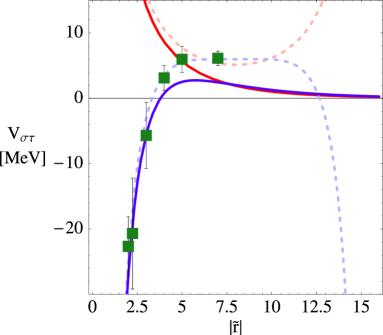
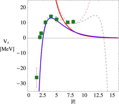
Figure 12: Fits to the finite-volume isovector $t$-channel potentials. The dashed lines correspond to the finite-volume fits to the lattice data, and the solid curves are the infinite-volume extrapolations.

If the couplings $\alpha_{\chi}^{(\prime)}$ in Eqs.(35) and (36) are included as fit parameters, we obtain instead

$$g_{\rho}=3.02\pm 0.09\,, g=0.69\pm 0.03\,,$$ (38)

with the finite-volume fits and their infinite-volume reconstructions shown as the dashed- and solid- blue curves in Fig. 12. In this case we have set the minimum separation, $r_{\rm min}$, used in our fits to be $2b$ for $V_{\sigma\tau}$ and $3b$ for $V_{\tau}$ although the fits vary only slightly under changes of $r_{\rm min}$ from $b$ to $5b$. Averaging the two sets of extractions, we find

$$g_{\rho}=2.6\pm 0.1\pm 0.4\,, g=0.63\pm 0.05\pm 0.06\,,$$ (39)

where the second error is an estimate of systematic errors determined by differences between the two fits and variation of the fit range. These numbers represent our best estimates of the couplings but we caution that we are currently unable to investigate the full systematics of this determination. Further refinement would require lattice calculations at a range of different volumes, lattice spacings and quark masses.

In both isovector channels, the agreement of the two infinite-volume extractions at large separations suggests that the long range piece of the extraction is robust. The pion coupling, $g$, is related to the forward limit of $\langle B|\ j^{a}_{\mu 5}\ |B^{\ast}\rangle$, the matrix element of the isovector axial-vector current, through PCAC and the value we extract is consistent with direct determinations of the quenched axial coupling: 0.42(4)(8) deDivitiis:1998kj , 0.69(18) Abada:2002xe , 0.48(3)(11) Abada:2003un , 0.517(16) Negishi:2006sc . We note that extraction of this coupling from the potential does not require renormalisation of axial current and suffers from different systematic effects. Agreement between the two procedures is encouraging.

The isoscalar channels suffer from more severe unphysical artefacts in quenched QCD and we are not able to extract meaningful information from the long distance potentials. For $V_{\sigma}$, EFT predicts a long range single Goldstone boson exchange potential Beane:2002nu

$$V_{\sigma}^{(\infty)}(|{\bf r}|) \stackrel{{\scriptstyle|{\bf r}|\to\infty}}{{\longrightarrow}} \frac{g_{0}^{2}\ m_{\pi}^{2}}{24\pi f_{\pi}^{2}}\left[(1-\alpha_{\Phi})\frac{e^{-m_{\pi}|{\bf r}|}}{|{\bf r}|}-\frac{M_{0}^{2}-\alpha_{\Phi}m_{\pi}^{2}}{2m_{\pi}}e^{-m_{\pi}|{\bf r}|}\right]$$ (40)

($g_{0}$ is the $\eta^{\prime}$ axial-coupling occurring in the quenched heavy-meson chiral Lagrangian Booth:1994hx ; Sharpe:1995qp ) with a long distance exponential tail dominating. Unlike the other channels, the suppression of the sub-leading contribution is not exponential and our data is insufficient to resolve these pieces. $V_{1}$ is not determined by single particle exchange (though many phenomenological approaches in the nucleon sector include exchange of the $\sigma(550)$ resonance) and in this channel our data are particularly poor. In both isoscalar channels two-$\eta^{\prime}$ exchange is also present and enhanced compared to two-pion, and one-$\eta^{\prime}$–one-pion- exchange, further polluting the signals. Larger volumes and multiple quark masses will be needed to perform extractions of couplings in these channels.

VI Discussion

We have studied the potentials between two $B$-mesons in the heavy quark limit. The calculations were performed on $16^{3}\times 32$ quenched lattices with a spatial length of $\sim 1.6~{}{\rm fm}$, and with a quark mass such that $m_{\pi}\sim 400~{}{\rm MeV}$. The leading lattice space corrections to the one-gluon-exchange potential between the two heavy quark propagators in the finite-volume were included in order to extract the physical potential between $B$-mesons in the continuum but at finite-volume. We find clear evidence of repulsion between the $B$-mesons in the $I\neq s_{l}$ channels and attraction in the $I=s_{l}$ channels. Three of the four potentials defined with $t$-channel spin-isospin quantum numbers have significantly smaller uncertainties than the potentials defined with $s$-channel quantum numbers. From the large separation behaviour of these potentials at finite-volume, $B$-meson couplings to the $\pi$ and $\rho$ were extracted.

This calculation can be improved in a number of areas but shows that a rigorous first principles calculation of the $B$-meson potential is achievable in the near future. The next stage of our study will progress from unphysical quenched QCD to fully dynamical QCD. This is mandatory for connection to the real world but will also significantly simplify the analysis of the long range potential using EFT. To separate the different components of the potential in the short-, intermediate- and long- range regimes requires multiple volumes and quark masses. Finally calculations at a number of different lattice spacing are required to control the remaining discretisation effects. Completion of this ambitious program will provide deep insight into the $BB$ system and, ultimately, nuclei.

Appendix A Potentials from Lattice Wavefunctions

Recently, it has been claimed that the nucleon-nucleon potential can be extracted from the lattice wavefunctions of two nucleons Ishii:2006ec , extending the technique that CP-PACS has successfully used to determine $I=2$ $\pi\pi$ scattering parameters Aoki:2005uf . In this appendix, we question the validity of that calculation.

An interpolating field for the nucleon is,

$$\hat{\cal O}_{1}({\bf x},t)_{\alpha}^{i} = \epsilon_{abc}\ q^{i,c}_{\alpha}\ \left(q^{a,T}C\gamma_{5}\tau_{2}q^{b}\right)({\bf x},t)\ \ \ ,$$ (41)

where $i$ is a Dirac-index, $\alpha$ is an isospin index, and $a,b,c$ are color indices. This operator has a non-zero overlap with a nucleon momentum-eigenstate

$$\langle 0|\hat{\cal O}_{1}({\bf 0},0)_{\alpha}^{i}|N_{\beta}^{j}({\bf p})\rangle = Z_{N}({\bf p})\ \delta_{\alpha\beta}\ \delta^{ij}\ \ \ .$$ (42)

The two-nucleon correlation function measured on the lattice in Ref. Ishii:2006ec is

$$G_{NN}({\bf x},{\bf y},t) = \langle 0|\hat{\cal O}_{1}({\bf x},t)_{\alpha}^{i}\hat{\cal O}_{1}({\bf y},t)_{\beta}^{j}\overline{J}(0)|0\rangle$$ (43)

$$= \sum_{n}\ \langle 0|\hat{\cal O}_{1}({\bf x},0)_{\alpha}^{i}\hat{\cal O}_{1}({\bf y},0)_{\beta}^{j}|\psi_{n}\rangle\langle\psi_{n}|\overline{J}(0)|0\rangle\ {e^{-E_{n}t}\over 2E_{n}}\ \ \ ,$$

where $\overline{J}$ is a wall-source on the initial time-slice $t_{0}=0$, and $|\psi_{n}\rangle$ are the eigenstates of the Hamiltonian in the finite-volume. In particular, $|\psi_{n}\rangle$ are states of definite baryon number ($B=2$), isospin and transformation under the hyper-cubic group. Setting $\langle\psi_{n}|\overline{J}(t_{0})|0\rangle=A_{n}(t_{0})$, at long times the correlation function becomes

$$G_{NN}({\bf x},{\bf y},t) \rightarrow A_{0}(0)\ \langle 0|\hat{\cal O}_{1}({\bf x},0)_{\alpha}^{i}\hat{\cal O}_{1}({\bf y},0)_{\beta}^{j}|\psi_{0}\rangle\ {e^{-E_{0}t}\over 2E_{0}}\ \ \ ,$$ (44)

and Ref. Ishii:2006ec asserts that $\langle 0|\hat{\cal O}_{1}({\bf x},t_{0})_{\alpha}^{i}\hat{\cal O}_{1}({\bf y},t_{0})_{\beta}^{j}|\psi_{0}\rangle=\langle 0|N({\bf x},t_{0})_{\alpha}^{i}N({\bf y},t_{0})_{\beta}^{j}|\psi_{0}\rangle\equiv\Phi^{ij}_{\alpha\beta}$ is the Bethe-Salpeter wavefunction (their Eq. (4)). From this definition, they generate a nucleon-nucleon potential via

$$V(r) = E\ +\ {1\over 2\mu}{\nabla^{2}G_{NN}\over G_{NN}}\ =\ E\ +\ {1\over 2\mu}{\nabla^{2}\Phi_{NN}\over\Phi_{NN}}\ \ \ ,$$ (45)

where $\Phi_{NN}$ is the projection of the Bethe-Salpeter wavefunction onto definite isospin and transformation under the hyper-cubic group. $\mu$ is the reduced mass of the two-nucleon system. However, this identification of the Bethe-Salpeter wavefunction is incorrect and the most general form for the matrix element is

$$\langle 0|\hat{\cal O}_{1}({\bf x},t_{0})_{\alpha}^{i}\hat{\cal O}_{1}({\bf y},t_{0})_{\beta}^{j}|\psi_{0}\rangle = Z_{NN}^{(S,I)}(|{\bf r}|)\ \langle 0|N({\bf x},t_{0})_{\alpha}^{i}N({\bf y},t_{0})_{\beta}^{j}|\psi_{0}\rangle+\ldots\,,$$ (46)

where $Z_{NN}^{(S,I)}(|{\bf r}|)$ is an unknown function that depends upon the spin, isospin and structure of the composite sink, $\hat{\cal O}_{1}({\bf x},t_{0})_{\alpha}^{i}\hat{\cal O}_{1}({\bf y},t_{0})_{\beta}^{j}$, and where ${\bf r}={\bf x}-{\bf y}$. The ellipsis denotes additional contributions from the tower of states of the same global quantum numbers. With this complete form of the matrix element, it is not possible to determine the potential from $G_{NN}$ without additional information. In the limit $|{\bf r}|\to\infty$, $Z_{NN}^{(S,I)}(|{\bf r}|)\to 1$ and the additional terms in Eq. (46) containing $p>2$ particles are suppressed. Consequently the scattering parameters can be rigorously extracted as has been done for the case of the pion Aoki:2005uf .

Appendix B Finite Lattice Spacing Correction to the Potential

The finite lattice spacing correction to the potential (in the $\overline{\bf 3}$ color channel) is given by,

$$\delta V_{QQ;\overline{\bf 3}}^{(L)}({\bf r}) = -{\overline{\alpha}(\mu)\over 3\pi^{2}b}\ \left({2\pi\over\tilde{L}}\right)^{3}\ \left[\ \left({\tilde{L}\over 2\pi}\right)^{2}\sum_{\bf n}^{\infty}\ \ \frac{e^{i2\pi{\bf n}\cdot\tilde{\bf r}/\tilde{L}}}{|{\bf n}|^{2}}\ -\ \sum_{{\bf n}}^{|n_{i}|\leq{\tilde{L}\over 2}}\ e^{i2\pi{\bf n}\cdot\tilde{\bf r}/\tilde{L}}\ G_{00}\left(\hat{n}_{x},\hat{n}_{y},\hat{n}_{z},0\right)\ \right]\,,$$

arising from the difference between continuum and lattice one gluon exchange evaluated at finite-volume.

The lattice contribution to this expression is simple to evaluate for the DBW2 action (the full form of the improved gluon propagator is given in Ref. Weisz:1983bn ), however calculating the continuum contribution is somewhat subtle. Difficulties arise in both the infrared and ultraviolet regimes. Both the lattice and continuum finite-volume sums are IR divergent, however provided both are regulated in the same way a sensible result ensues; the simplest procedure is to omit the zero-mode.

While the continuum contributions to ${\cal A}$ and ${\cal B}$, defined in Eq. (29), are strictly UV convergent, that convergence is highly oscillatory. Computing these contributions is simplified by the use of the Poisson summation formula which allows the sum to be rewritten as

$$\sum_{{\bf n}\neq 0}\frac{e^{2\pi i{\bf n}\cdot\tilde{\bf r}/\tilde{L}}}{|{\bf n}|^{2}} = x^{2}\sum_{{\bf n}\neq 0}\frac{e^{2\pi i{\bf n}\cdot\tilde{\bf r}/\tilde{L}}}{|{\bf n}|^{2}(|{\bf n}|^{2}+x^{2})}+\sum_{{\bf n}\neq 0}\frac{e^{2\pi i{\bf n}\cdot\tilde{\bf r}/\tilde{L}}}{(|{\bf n}|^{2}+x^{2})}$$ (48)

$$= x^{2}\sum_{{\bf n}\neq 0}\frac{e^{2\pi i{\bf n}\cdot\tilde{\bf r}/\tilde{L}}}{|{\bf n}|^{2}(|{\bf n}|^{2}+x^{2})}-\frac{1}{x^{2}}+\frac{L\pi}{|\tilde{{\bf r}}|}e^{-2\pi x|\tilde{{\bf r}}|/L}+\pi\sum_{{\bf m}\neq 0}\frac{e^{-2\pi|{\bf m}+\tilde{{\bf r}}/\tilde{L}|x}}{|{\bf m}+\tilde{{\bf r}}/\tilde{L}|}\ \ \ ,$$

which is independent of the value of $x$. The sums on the rhs of this expression are more convergent than that on the lhs and can be numerically evaluated reliably. Similar techniques allowed us to deal with the analogous differences defining the function ${\cal B}$.

In the limit that $|\tilde{\bf r}|\to 0$, the continuum contribution is singular, leading to a correction factor of

$$\delta V_{QQ;\overline{\bf 3}}^{(L)}({\bf r}) \rightarrow -{2\ \overline{\alpha}(\mu)\over 3\ r}\ +\ ...\ \ \ ,$$ (49)

which is nothing other than the strong Coulomb interaction between the heavy quarks in the continuum. In the continuum limit and infinite-volume limit, $b\ll r\ll L$, the leading correction factor is found to be

$$\delta V_{QQ;\overline{\bf 3}}^{(L)}({\bf r}) \rightarrow -\frac{\overline{\alpha}(r^{-1})\ b^{2}}{6\ r^{3}}\left(1+12c_{1}-12c_{1}^{3}\right)\ +\ \ldots\,,$$ (50)

where we have used the BLM procedure to set the scale. This improved perturbative shift can be eliminated for suitable choices of $c_{1}$. Clearly, the Lüscher-Weisz-improved value of $c_{1}={1\over 12}$ maximally improves the lattice calculation. That is to say that, neglecting the small $c_{1}^{3}$ contribution, the correction factor that must be applied to the lattice calculation in order to recover the continuum potentials is minimized by Lüscher-Weisz-improvement.

References

• (1) S. C. Pieper and R. B. Wiringa, Ann. Rev. Nucl. Part. Sci.  51, 53 (2001) [arXiv:nucl-th/0103005].
• (2) P. Navratil, V. G. Gueorguiev, J. P. Vary, W. E. Ormand and A. Nogga, arXiv:nucl-th/0701038.
• (3) S. R. Beane, P. F. Bedaque, W. C. Haxton, D. R. Phillips and M. J. Savage, “From hadrons to nuclei: Crossing the border”, published in the Handbook of QCD, edited by M. Shifman (World Scientific Publishing) 2001. ISBD-981-02-4445-2. [arXiv:nucl-th/0008064].
• (4) P. F. Bedaque and U. van Kolck, Ann. Rev. Nucl. Part. Sci.  52, 339 (2002) [arXiv:nucl-th/0203055].
• (5) S. R. Beane, P. F. Bedaque, K. Orginos and M. J. Savage, Phys. Rev. Lett.  97, 012001 (2006) [arXiv:hep-lat/0602010].
• (6) S. R. Beane, P. F. Bedaque, T. C. Luu, K. Orginos, E. Pallante, A. Parreno and M. J. Savage [NPLQCD Collaboration], arXiv:hep-lat/0612026.
• (7) M. Lüscher, Commun. Math. Phys.  105, 153 (1986).
• (8) M. Lüscher, Nucl. Phys.  B 354, 531 (1991).
• (9) N. Isgur and M. B. Wise, Phys. Lett.  B 232, 113 (1989).
• (10) N. Isgur and M. B. Wise, Phys. Lett.  B 237, 527 (1990).
• (11) E. Eichten and B. R. Hill, Phys. Lett.  B 234, 511 (1990).
• (12) H. Georgi, Phys. Lett.  B 240, 447 (1990).
• (13) D. G. Richards, D. K. Sinclair and D. W. Sivers, Phys. Rev.  D 42, 3191 (1990).
• (14) A. Mihály, H. R. Fiebig, H. Markum and K. Rabitsch, Phys. Rev.  D 55, 3077 (1997).
• (15) C. Stewart and R. Koniuk, Phys. Rev.  D 57, 5581 (1998) [arXiv:hep-lat/9803003].
• (16) C. Michael and P. Pennanen [UKQCD Collaboration], Phys. Rev.  D 60, 054012 (1999) [arXiv:hep-lat/9901007].
• (17) P. Pennanen, C. Michael and A. M. Green [UKQCD Collaboration], Nucl. Phys. Proc. Suppl.  83, 200 (2000) arXiv:hep-lat/9908032.
• (18) A. M. Green, J. Koponen and P. Pennanen, Phys. Rev. D 61, 014014 (2000) [arXiv:hep-ph/9902249].
• (19) H. R. Fiebig [LHP collaboration], Nucl. Phys. Proc. Suppl.  106, 344 (2002) [arXiv:hep-lat/0110163].
• (20) H. R. Fiebig [LHP Collaboration], Nucl. Phys. Proc. Suppl.  109A, 207 (2002) [arXiv:hep-lat/0112010].
• (21) M. S. Cook and H. R. Fiebig, arXiv:hep-lat/0210054.
• (22) T. T. Takahashi, T. Doi and H. Suganuma, AIP Conf. Proc.  842, 249 (2006) [arXiv:hep-lat/0601006].
• (23) T. Doi, T. T. Takahashi and H. Suganuma, AIP Conf. Proc.  842, 246 (2006) [arXiv:hep-lat/0601008].
• (24) S. R. Beane and M. J. Savage, Phys. Lett.  B 535, 177 (2002) [arXiv:hep-lat/0202013].
• (25) T. Takaishi, Phys. Rev.  D 54, 1050 (1996).
• (26) P. de Forcrand et al. [QCD-TARO Collaboration], Nucl. Phys.  B 577, 263 (2000) [arXiv:hep-lat/9911033].
• (27) Y. Aoki et al., Phys. Rev.  D 69, 074504 (2004) [arXiv:hep-lat/0211023].
• (28) G. Colangelo and S. Durr, Eur. Phys. J.  C 33, 543 (2004) [arXiv:hep-lat/0311023].
• (29) A. F. Falk, M. Neubert and M. E. Luke, Nucl. Phys.  B 388, 363 (1992) [arXiv:hep-ph/9204229].
• (30) A. Duncan, E. Eichten, J. Flynn, B. R. Hill, G. Hockney and H. Thacker, Phys. Rev.  D 51, 5101 (1995) [arXiv:hep-lat/9407025].
• (31) G. Martinelli and C. T. Sachrajda, Nucl. Phys.  B 559, 429 (1999) [arXiv:hep-lat/9812001].
• (32) M. Lüscher and P. Weisz, Commun. Math. Phys.  97, 59 (1985) [Erratum-ibid.  98, 433 (1985)].
• (33) M. Lüscher and P. Weisz, Phys. Lett.  B 158, 250 (1985).
• (34) Y. Iwasaki, preprint UTHEP-118 (Dec 1983), unpublished.
• (35) P. Weisz and R. Wohlert, Nucl. Phys.  B 236, 397 (1984) [Erratum-ibid.  B 247, 544 (1984)].
• (36) S. Capitani, Phys. Rept.  382, 113 (2003) [arXiv:hep-lat/0211036].
• (37) S. Aoki, T. Izubuchi, Y. Kuramashi and Y. Taniguchi, Phys. Rev.  D 67, 094502 (2003) [arXiv:hep-lat/0206013].
• (38) S. J. Brodsky, G. P. Lepage and P. B. Mackenzie, Phys. Rev.  D 28, 228 (1983).
• (39) F. Wilczek and A. Zee, Phys. Rev.  D 16, 860 (1977).
• (40) G. Karl, Phys. Rev.  D 14, 2374 (1976).
• (41) W. J. Marciano, Phys. Rev.  D 21, 2425 (1980).
• (42) J. E. Mandula, G. Zweig and J. Govaerts, Nucl. Phys.  B 228, 91 (1983).
• (43) N. Kaiser, R. Brockmann and W. Weise, Nucl. Phys.  A 625, 758 (1997) [arXiv:nucl-th/9706045].
• (44) G. Burdman and J. F. Donoghue, Phys. Lett.  B 280, 287 (1992).
• (45) M. B. Wise, Phys. Rev.  D 45, 2188 (1992).
• (46) T. M. Yan, H. Y. Cheng, C. Y. Cheung, G. L. Lin, Y. C. Lin and H. L. Yu, Phys. Rev.  D 46, 1148 (1992) [Erratum-ibid.  D 55, 5851 (1997)].
• (47) M. J. Booth, Phys. Rev.  D 51, 2338 (1995) [arXiv:hep-ph/9411433].
• (48) S. R. Sharpe and Y. Zhang, Phys. Rev.  D 53, 5125 (1996) [arXiv:hep-lat/9510037].
• (49) C. W. Bernard and M. F. L. Golterman, Phys. Rev.  D 46, 853 (1992) [arXiv:hep-lat/9204007].
• (50) S. R. Sharpe, Phys. Rev.  D 46, 3146 (1992) [arXiv:hep-lat/9205020].
• (51) G. M. de Divitiis, L. Del Debbio, M. Di Pierro, J. M. Flynn, C. Michael and J. Peisa [UKQCD Collaboration], JHEP 9810, 010 (1998) [arXiv:hep-lat/9807032].
• (52) A. Abada et al., Phys. Rev.  D 66, 074504 (2002) [arXiv:hep-ph/0206237].
• (53) A. Abada, D. Becirevic, Ph. Boucaud, G. Herdoiza, J. P. Leroy, A. Le Yaouanc and O. Pene, JHEP 0402, 016 (2004) [arXiv:hep-lat/0310050].
• (54) S. Negishi, H. Matsufuru and T. Onogi, Prog. Theor. Phys.  117, 275 (2007) [arXiv:hep-lat/0612029].
• (55) R. G. Edwards and B. Joo Nucl. Phys. Proc. Suppl.  140, 832 (2005) [arXiv:hep-lat/0409003].
• (56) N. Ishii, S. Aoki and T. Hatsuda, arXiv:nucl-th/0611096.
• (57) S. Aoki et al. [CP-PACS Collaboration], Phys. Rev.  D 71, 094504 (2005) [arXiv:hep-lat/0503025].