Continuum limit of string formation in 3-d SU(2) LGT

Abstract:

We study the continuum limit of the string-like behaviour of flux tubes formed between static quarks and anti-quarks in three dimensional $SU(2)$ lattice gauge theory. We compare our simulation data with the predictions of both effective string models as well as perturbation theory. On the string side we obtain clear evidence for convergence of data to predictions of Nambu-Goto theory. We comment on the scales at which the static potential starts departing from one loop perturbation theory and then again being well described by effective string theories. We also estimate the leading corrections to the one-loop perturbative potential as well as the Nambu-Goto effective string. In the intermediate regions we find that a modified Lennard-Jones type potential gives surprisingly good fits.

1 Introduction

Gluonic dynamics at large distances can be very effectively probed by looking at properties of the flux tube which forms between a static quark and an anti-quark in the QCD vacuum. Although there is still no analytical proof of this formation, lattice simulation results overwhelmingly indicate that this indeed is the case [1].

Bosonic string descriptions of this flux tube have been around for a long time. While most of the earlier attempts [2] used an open string description with the ends of the string ending on the quark and the anti-quark, recently there have been attempts to give closed string descriptions too. After Polchinski and Strominger(PS) [3] suggested how effective theory of strings with vanishing conformal anomaly could be formulated in all dimensions it has been shown [4, 5, 6] that the spectrum of these effective theories is universal to order $r^{-3}$ ($r$ being the length of the string) and that to this order they coincide with the predictions of Nambu-Goto theory whose conformal anomaly however vanishes only in 26 dimensions.

Another interesting idea put forward by Lüscher and Weisz [7] is that of open-closed string duality. They showed that this too constrained the possible string spectra. In three dimensions they found that this duality implied that to order $r^{-3}$ the spectrum was the same as that of the Nambu-Goto(NG) string while in four dimensions one parameter was left undetermined. In the PS effective string theories the spectrum to this order is the same as NG theory in all dimensions without needing to invoke open-closed duality explicitly.

On the lattice, the flux tube can be observed as the potential between a static quark and an anti-quark (open string). This can be obtained from expectation values of Wilson loops or Polyakov loop correlators. One of the characteristics of the string like behaviour of the flux tube is the presence of a long distance $1/r$ term in all dimensions and with a universal coefficient in the $q\bar{q}$ potential. In four dimensions there is a short distance $1/r\log(r)$ term in the potential. However its coefficient depends on the details of the gauge group distinguishing it from the long distance $1/r$ term. The long distance $1/r$ term was first observed in [8] and its universality was established in [9]. It is known as the Lüscher term.

The Lüscher term has been looked at in lattice simulations since the eighties [10, 11]. However in recent times, increase in computing power and improvement in algorithms have allowed really precise measurements of that term and also the $r^{-3}$ term. Now it is possible to study the properties of flux tubes longer than 1 fermi which was unimaginable even a few years back and one is really in a position to compare the lattice data with the predictions of the string picture. See [12, 13, 14, 15, 16, 17, 18, 19, 20] for example. In particular, measurements of the Lüscher term in three dimensions have been carried out in [17, 19] for $SU(2)$ , in [14] for $SU(3)$ and in [18] for $SU(5)$ lattice gauge theories. Convergence to the static potential of NG theory to order $r^{-3}$ at a distance scale of around 1 fermi has been recently shown in the case of $d=4$ $SU(3)$ gauge theories in [15].

Another characteristic of the string behaviour of the flux tube is the level spacing of the excitation spectrum. We do not discuss it here. See [7, 16, 17, 21, 22] for recent analytic and numerical studies. A review on this topic can also be found in [23].

In this article we present results of our simulations of the Polyakov loop correlators for $d=3$ $SU(2)$ Yang-Mills theory and compare the resulting static potential with both perturbation theory and string model predictions. This allows us to narrow down bounds on the distance beyond which we can say the flux tube indeed shows a string like behaviour.

2 Simulation parameters

We have carried out simulations of three dimensional $SU(2)$ lattice gauge theory on lattices at four different lattice spacings with the coarsest lattice having a spacing of slightly below 0.13 fm to the finest lattice with a spacing of about 0.045 fermi. We use symmetric cubic lattices and the Wilson gauge action. On all these lattices, we have computed Polyakov loop correlators $\langle P^{*}(x)P(y)\rangle$ for various spatial separations $r=y-x$.

To reliably extract signals of these observables which are exponentially decreasing functions of $r$ and $T$ (the temporal extent of the lattice), we used the Lüscher-Weisz exponential error reduction algorithm [13]. In this algorithm, one computes intermediate expectation values on sub-lattices of the original lattice which are obtained by imposing suitable boundary conditions. For measuring Polyakov loop correlators, we obtain our sub-lattices by slicing the original lattice along the temporal direction. As is well known, this algorithm has several optimization parameters among which the number of sub-lattice updates employed seems to be the most important one. The lattice parameters along with the number of sub-lattice updates used in each set of measurements are summarized in table 1.

Table 1: Runs

$\beta$	$r$ values	lattice	iupd	$\#$ of measurements
5.0	$~{}2-8~{}$	$36^{3}$	16000	1600
	$~{}7-9~{}$	$40^{3}$	32000	3200
	$~{}8-12$	$48^{3}$	48000	7000
7.5	$~{}4-8~{}$	$48^{3}$	8000	1100
	$~{}7-12$	$64^{3}$	18000	1100
	$11-16$	$64^{3}$	36000	7200
10.0	$~{}2-7~{}$	$48^{3}$	16000	2850
	$~{}6-9~{}$	$48^{3}$	16000	200
	$~{}8-14$	$84^{3}$	24000	1100
	$13-19$	$84^{3}$	36000	2250
12.5	$~{}2-9~{}$	$48^{3}$	16000	2700
	$~{}8-14$	$72^{3}$	24000	1150

Another important parameter is the thickness of the time-slice over which the sub-lattice averages are carried out. We found that it was helpful to increase this thickness as one goes from stronger to weaker coupling. We used values of two, four and six as time-slice thicknesses.

To optimize the running time while keeping any finite volume effect under control we chose different lattice sizes for different ranges of $r$. Typically the smaller values of $r$ are much easier to get as they can be reliably obtained on smaller lattices and require much less sub-lattice updates. In principle of course results for all the different $r$ values could be obtained from the largest lattice but memory requirements prevent us from doing all the measurements in a single run.

Table 2: Lattice scales

$\beta$	$\frac{1}{2}\langle{\rm Tr}~{}u_{P}\rangle$	$~{}~{}a^{2}\sigma$	$r_{0}~{}~{}~{}~{}~{}~{}$	$a~{}(fm)$	$\quad\sigma r_{0}^{2}$
5.0	0.786878 (7)	0.097334  (6)	$3.9536~{}~{}(3)$	0.12648  (2)	1.5214  (3)
7.5	0.861665 (4)	0.038566  (6)	$6.2875~{}(10)$	0.07952  (1)	1.5246  (7)
10.0	0.897683 (3)	0.020606  (4)	$8.6022~{}~{}(8)$	0.05812  (1)	1.5248  (4)
12.5	0.921100 (2)	0.012742 (17)	$10.916~{}~{}~{}(3)$	0.04580  (1)	1.5215 (29)

The scale is set by the Sommer scale $r_{0}=0.5~{}{\rm fm}$ which is implicitly defined by $r_{0}^{2}f(r_{0})=1.65$, where $f(r)$ is the force between the static quark and the anti-quark. We use our measured force values and interpolation to extract $r_{0}$. The values that we obtain are given in table 2. We also see from table 2 that $\sigma r_{0}^{2}$ is a constant $(\simeq 1.522)$ to a very good approximation as expected in the scaling region close to the continuum limit.

3 Results

In this section we present the results of our measurements. From the $\langle P^{*}P\rangle$ correlator one can extract the static quark-antiquark potential $V(r)$ by

$$V(r)=-\frac{1}{T}\ln\langle P^{*}P(r)\rangle.$$ (1)

In principle the $q\bar{q}$ potential contains all the information about the flux tube, but it also contains an unphysical constant. We therefore look directly at the first and the second derivative of this potential.

The first derivative of the potential gives us the force between the quark and the antiquark, while the second derivative gives us information about the subleading terms and how one approaches the asymptotic linearly rising behaviour of the $q\bar{q}$ potential. To facilitate our comparison with string models we actually compute a scaled second derivative which we call $c(\tilde{r})$. This quantity should become the Lüscher term ($=-\frac{(d-2)\pi}{24}$) asymptotically.

On the lattice these quantities are given by

$$F({\bar{r}}) = V(r)-V(r-1)$$ (2)

$$c({\tilde{r}}) = \frac{{\tilde{r}}^{3}}{2}[V(r+1)+V(r-1)-2V(r)]$$ (3)

where ${\bar{r}}=r+\frac{a}{2}+{\cal O}(a^{2})$ and ${\tilde{r}}=r+{\cal O}(a^{2})$ are defined as in [14] to reduce lattice artifacts.

The theoretical predictions in continuum are given by string models (for large $r$) as well as perturbation theory (for small $r$). Since non-bosonic string models have been essentially ruled out [24], we are going to concentrate on the potential due to the NG string, the so called Arvis potential [25] given by

$$V_{\rm Arvis}=\sigma r\left(1-\frac{(d-2)\pi}{12\sigma r^{2}}\right)^{1/2}.$$ (4)

Keeping in mind the results of Lüscher and Weisz [7] and PS type effective string theories [4, 5, 6] we are going to compare our lattice data on force and $c(r)$ with leading order predictions to which all models reduce at sufficiently large $r$, to NLO expressions and expressions from the full Arvis potential. In three dimensions the expressions are given by

$${\bf L.O.}\quad f(r) = \sigma+\left(\frac{\pi}{24}\right)\frac{1}{r^{2}}\qquad\qquad\qquad\qquad~{}~{}~{}c(r)=-\frac{\pi}{24}$$

$${\bf N.L.O.}\quad f(r) = \sigma+\left(\frac{\pi}{24}\right)\frac{1}{r^{2}}+\left(\frac{\pi}{24}\right)^{2}\frac{3}{2\sigma r^{4}}\qquad~{}c(r)=-\frac{\pi}{24}\left(1+\frac{\pi}{8\sigma r^{2}}\right)$$

$${\rm Arvis}\quad f(r) = \sigma\left(1-\frac{\pi}{12\sigma r^{2}}\right)^{-1/2}\qquad\qquad\qquad c(r)=-\frac{\pi}{24}\left(1-\frac{\pi}{12\sigma r^{2}}\right)^{-\frac{3}{2}}.$$ (5)

The perturbative potential has been calculated at the one loop level by Schröder [26]. He obtains

$$V_{\rm pert}(r)=\sigma_{\rm pert}r+\frac{g^{2}C_{F}}{2\pi}\ln g^{2}r+(\rm higher~{}order~{}terms)\\$$ (6)

with the perturbative string tension $\sigma_{\rm pert}=\frac{7g^{4}C_{F}C_{A}}{64\pi}$. For $SU(2)$ $C_{F}=3/4$, $C_{A}=2$. The perturbative force and $c_{\rm pert}(r)$ can be computed by $f_{\rm pert}(r)=\frac{dV_{\rm pert}(r)}{dr}$ and $c_{\rm pert}(r)=\frac{r^{3}}{2}\frac{d^{2}V_{\rm pert}(r)}{dr^{2}}.$

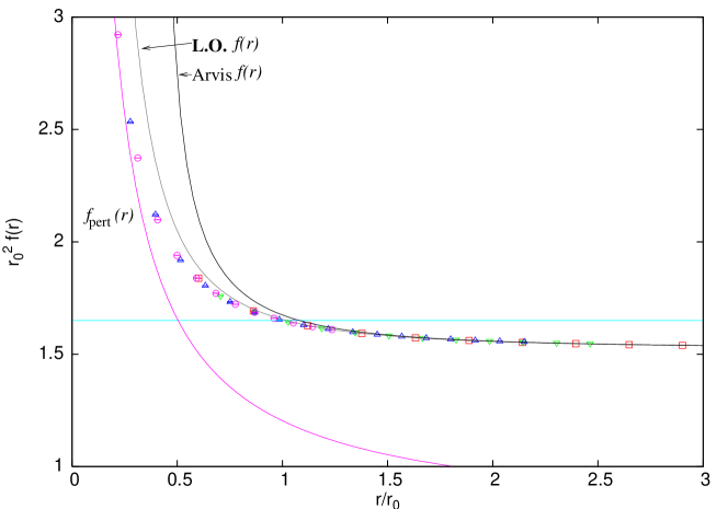
Figure 1: $r_{0}^{2}f(r)$ vs $r/r_{0}$ in the $d=3$ $SU(2)$ case. The four different sets are $\square~{}(\beta=5)$, $\bigtriangledown~{}(\beta=7.5)$, $\bigtriangleup~{}(\beta=10)$ and $\bigcirc~{}(\beta=12.5)$. Also shown is the 1-loop perturbation theory curve $f_{\rm pert}(r)$, as well as the leading order (L.O. $f(r)$) and NG (Arvis $f(r)$) string predictions. The horizontal line is $r_{0}^{2}f(r)=1.65$ and locates the Sommer scale.

We first look at the force data. Since we have four values of the coupling, we look at the continuum limit of the string tension. Following [27] we too define $\beta_{\rm MF}=\beta\times\frac{1}{2}\langle{\rm Tr}~{}u_{P}\rangle$ and look at how $a\sqrt{\sigma}$ scales with $\beta_{\rm MF}$. We use $\beta_{\rm MF}=4/g^{2}a$ to convert the perturbative expressions to lattice units. Fitting the string tension to the form

$$a\sqrt{\sigma}=\frac{8}{\beta_{\rm MF}}\left(\frac{\sqrt{\sigma}}{g^{2}N}\right)_{\rm cont.}+\frac{a_{1}}{\beta_{\rm MF}^{2}}+\frac{a_{2}}{\beta_{\rm MF}^{3}},$$ (7)

where $N$ refers to the gauge group $SU(N)$, we obtain $\left(\frac{\sqrt{\sigma}}{g^{2}N}\right)_{\rm cont.}$, for $N=2$, to be 0.16788(12) which is completely consistent with the values presented in [27, 28]. As noted by Schröder [26], the full string tension is 1.47 times the perturbative string tension and hardly changes for $N$ between 2 and 5. We want to also mention that if we ignore the point $\beta=5$, then the data can be well described even without the coefficient $a_{2}$. In that case we obtain the continuum value to be 0.16736(10). Another point worth noting is that while we too find the coefficient $a_{1}$ to be negative, in agreement with [27], the coefficient $a_{2}$ is positive in our case. This is consistent with the higher $N$’s in [27], and may not be of much significance as in that work, $a_{2}$ for $SU(2)$ is consistent with 0 within 2$\sigma$.

The values obtained for $\sigma r_{0}^{2}$ by fitting the force to the Arvis form is quoted in table 2. The values given by the other two forms differs by less than 0.1% from the quoted values. $\sigma r_{0}^{2}$ scales very nicely with the different beta values differing by less than 0.2% from each other. The fits were carried out in the range 2.4 - 2.9 $r_{0}$ for $\beta=5$ , 2.1 - 2.5 $r_{0}$ for $\beta=7.5$, 1.9 - 2.1 $r_{0}$ for $\beta=10$ and finally between 1.6 - 1.8 $r_{0}$ for $\beta=12.5$. The data for large $r$ at $\beta=12.5$ was taken from [17].

In Fig. 1 we plot $r_{0}^{2}f$ versus $r/r_{0}$ which is expected to become a universal curve in the continuum limit. The horizontal line is $r^{2}f(r)=1.65$ and defines the Sommer scale $r_{0}$. The grey line is the L.O. result $\sigma r_{0}^{2}+\frac{\pi}{24}\left(\frac{r_{0}}{r}\right)^{2}$ . The black line is the Arvis curve and the magenta one the perturbative curve. The data starts departing from the one-loop perturbative curve around 0.22 $r_{0}$ or 1.8 GeV and joins onto the string curves around 1.5 $r_{0}$ or 260 MeV. The scaling exhibited by the data is very good with all the four different beta values falling on the same curve. This is mainly due to use of $\overline{r}$ instead of $r$ , as it eliminates lattice artefacts to a large extent. The value for $\sigma r_{0}^{2}$ for drawing the L.O. and Arvis curves is taken from the fit at $\beta=5$ as it extends to the largest distance. Beyond 1.5$r_{0}$ it is virtually impossible to distinguish the different theoretical curves as they are all dominated by the universal leading order behaviour with the string tension making up more than 95% of the force. The force data in fact gives the wrong impression of the string description being good even at distances as small as $r_{0}$.

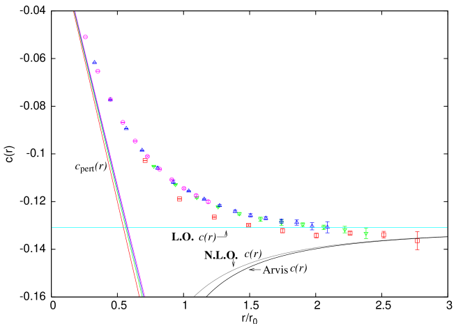
Figure 2: $c(\tilde{r})$ in $d=3$ $SU(2)$ case. The four different sets are $\square~{}(\beta=5)$, $\bigtriangledown~{}(\beta=7.5)$, $\bigtriangleup~{}(\beta=10)$ and $\bigcirc~{}(\beta=12.5)$. Also shown are 1-loop perturbation theory ($c_{\rm pert}(r)$), L.O., N.L.O. and NG (Arvis) string model predictions.

On the other hand, $c(\tilde{r})$ does not contain the string tension, and has a universal value in the L.O. It is therefore more sensitive to the sub-leading behaviour of the flux tube. In Fig. 2 we plot $c(\tilde{r})$ (versus $r$ in units of $r_{0}$) for all four $\beta$ values along with the perturbative curves as well as the three string model predictions given in eqn. 3. The line and the symbol $\square$ in red corresponds to $\beta=5$, while the symbols $\bigtriangledown$, $\bigtriangleup$ and $\bigcirc$ in colours green, blue and magenta correspond to the $\beta$ values 7.5, 10 and 12.5 respectively. The blue horizontal line corresponds to the leading order prediction while the ash and black curves correspond to the NLO and Arvis forms respectively. We look at a wide range of $r$ starting from where the data almost touches the perturbative curves going all the way to the region where the string predictions hold.

The data seems to lie on top of each other exhibiting nice scaling behaviour as one goes to larger values of $r$. The $\beta=12.5$ and $\beta=10$ data lie on top of each other in the range 0.75 and 1.25 $r_{0}$ already. The $\beta=7.5$ set joins onto this at around 1.5$r_{0}$ and even the $\beta=5$ data joins up at around 2.25$r_{0}$. This points to the possibility that the continuum limit of the scale where the flux tube is well described by the Arvis curve can be obtained already on relatively coarse lattices.

4 Discussions

In $d=3$, as also noted by Schröder, infrared divergences prevent computation of the perturbative potential beyond one loop. Infrared counterterms have to be obtained non-perturbatively . As our data goes down to distances of about 0.16 fermi, we can try to obtain these counter terms by looking at two loop terms in the perturbative potential. On dimensional grounds, one can expect the perturbative potential to be of the form

$$V_{\rm pert}(r)=\frac{g^{2}C_{F}}{2\pi}\ln g^{2}r+\frac{7C_{F}C_{A}g^{4}}{64\pi}r+Ag^{4}r\ln g^{2}r+Bg^{6}r^{2}+\cdots$$ (8)

This gives

$$c_{\rm pert}(r)=-\frac{g^{2}r_{0}C_{F}}{4\pi}\frac{r}{r_{0}}+\frac{Ag^{4}r_{0}^{2}}{2}\left(\frac{r}{r_{0}}\right)^{2}+Bg^{6}r_{0}^{3}\left(\frac{r}{r_{0}}\right)^{3}.$$ (9)

Since the first term is known, we determine $A$ and $B$ from the initial two points of our data to be $A=0.013162(3)$ and $B=0.001089(1)$. On our finest lattice we obtain $g^{2}r_{0}$, which is RG-invariant in the continuum limit, to be $3.792$. While $B$ contains effects of higher order terms, we expect the coefficient $A$ to be relatively well determined. From the ratio of the leading to the next to leading term in $V_{\rm pert}(r)$ as well as the data on $c({\tilde{r}})$, we estimate the range of validity of first order perturbation theory to be about $0.1$ fermi (consistent with our estimate from the force data). Fig. 3 suggests that second order perturbation theory holds upto distances of about $0.2$ fermi.

To try to get an idea about the scale of string formation, we look at the percentage of the total force carried by the string tension and the relative difference between the Arvis and the leading order force. From our data we find that the string tension constitutes 95% of the force at around 1.3$r_{0}$, 98% at around 2.1$r_{0}$ and 99% at around 2.9$r_{0}$. The relative difference, which gives us an idea about the importance of the subleading behaviour, is about 2% at 1.02$r_{0}$, 1% at 1.2$r_{0}$ and goes down to 0.1% at about 1.9$r_{0}$.

The type of string is even more difficult to identify. At leading order, a variety of theories with different boundary conditions yield the universal Lüscher term [29]. In fact all effective string theories of the PS type and AdS/CFT correspondences [30] also yield this term. The type is therefore determined by the sub-leading behaviour of the flux tube. What can be clearly seen in the data is that the approach to the Lüscher term is from below, consistent with effective bosonic string model predictions. At short distances the data matches perturbation theory. Therefore $c({\tilde{r}})$ crosses the asymptotic value at some intermediate point. For $SU(2)$, this intermediate point seems to be around 2$r_{0}$ or 1 fermi. Here it is still not clear whether a string behaviour has set in. It is only at a still larger distance of about 2.75$r_{0}$, that the data seems to be well described by the Arvis curve.

An interesting question is what happens to these scales for $SU(N)$ as $N$ increases. It has been observed in [18] that the intermediate $q\bar{q}$ separation at which $c(\tilde{r})$ assumes its asymptotic value decreases with increasing $N$ at finite lattice spacing. For $SU(3)$ the data on the coarsest lattice in ref. [14] just about touches the Arvis curve at 1.8$r_{0}$. However both these scales shift towards larger $r$ as one approaches the continuum limit.

Comparing the data with effective strings at higher orders may tell us if the scale of string formation is the one suggested by the Arvis curve or happens earlier. From ${\cal O}(r^{-4})$ and beyond, effective string theories motivate parametrising the leading deviations to $c(\tilde{r})$ from the Arvis behaviour as

$$\Delta c(\tilde{r})=A\left(\frac{r_{0}}{r}\right)^{4}+B\left(\frac{r_{0}}{r}\right)^{6}.$$ (10)

From our data in the region $1.6-2.4~{}r_{0}$ we obtain, as best fit values, $A=0.209(9),B=-0.235(24)$. The corresponding terms of the Arvis potential are $A_{\rm Arvis}=-0.00725,B_{\rm Arvis}=-0.00145$. It is of interest to know what the predictions of effective string theories are for these.

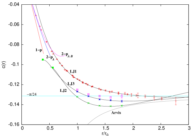
Figure 3: Curves of the type given in eqn. 11 describing the $c(\tilde{r})$ data in the intermediate region. The red + is the continuum limit $3-d\,SU(2)$ data. The green $\times$, the blue $\ast$ and the magenta $\square$ are $3-d\,SU(3)$ data from [14] with $r_{0}=3.30,4.83$ and $6.71$ respectively. The curves LJ1, LJ2 and LJ3 are given by $(a,b,n)$ of $(0.444,-0.258,0.357)$ , $(0.458,-0.289,0.691)$ and $(0.442,-0.287,0.498)$ respectively. The perturbative curves marked 1-p, 2-p_A and 2-p_AB are given by the first, the first two and all the three terms of the expression: $-\frac{g^{2}r_{0}C_{F}}{4\pi}\frac{r}{r_{0}}+\frac{Ag^{4}r_{0}^{2}}{2}\left(\frac{r}{r_{0}}\right)^{2}+Bg^{6}r_{0}^{3}\left(\frac{r}{r_{0}}\right)^{3}$ with $A=0.013162$ and $B=0.001089$. The green filled squares denote the smallest possible values of $r/r_{0}$ for which $c(\tilde{r})$ can be calculated on that particular lattice.

At intermediate distances over a wide region of $r$ varying from $0.5r_{0}$ to $2.8r_{0}$, the data is very well described by a formula of the type

$$c(\tilde{r})=a\left(\frac{1}{x^{2n}}-\frac{1}{x^{n}}+\frac{b}{x^{3n}}\right)$$ (11)

with $a=0.444(4),~{}b=-0.258(2)$ and $n=0.357(15)$. Existing $SU(3)$ data in 3-d [14] also admit a similar description with nearly same values of $a$ and $b$, but with a different $n$. The curves are shown in Fig. 3. At the moment it is not at all clear if there is any theoretical basis for such a description. However they certainly provide accurate interpolation formulae.

5 Conclusions

In this article we have looked at the continuum limit behaviour of the $SU(2)$ flux tube at intermediate distances by measuring the static $q\bar{q}$ potential. Starting from a distance of about 0.1 fermi where the potential starts breaking away from 1-loop perturbation theory, we go to distances of about 1.4 fermi where the data begins to be well described by the Arvis potential.

We look at the continuum limit of the string tension and find complete agreement between open and closed strings [27]. Our data on $c(\tilde{r})$ seems to approach the Lüscher term from below as expected in bosonic string models. At distances below 0.15 fermi the data joins onto the perturbative values. A modified Lennard-Jones type empirical formula describes the data well in the intermediate region.

Further directions of study include increasing the $q\bar{q}$ separation to confirm that the data indeed stays on the Arvis curve. For $SU(3)$ and $SU(5)$, it would be really interesting to push to the continuum limit to see if the behaviour seen in $SU(2)$ holds in those cases and find the distance where the data meets the Arvis curve.

Table 3: Force and $c(\tilde{r})$ ($\beta=5$)

$r$	$\overline{r}$	$f(r)$	$\tilde{r}$	$c(\tilde{r})$
3	2.3790	0.11744 (1)	2.808	$-$0.10274 (3)
4	3.4071	0.10816 (1)	3.838	$-$0.11886 (8)
5	4.4322	0.10395 (1)	4.876	$-$0.1265 (2)
6	5.4481	0.10177 (2)	5.903	$-$0.1299 (4)
7	6.4579	0.10051 (2)	6.920	$-$0.1322 (9)
8	7.4645	0.09974 (2)	7.932	$-$0.1342 (10)
9	8.4692	0.09919 (1)	8.941	$-$0.1330 (7)
10	9.4727	0.09883 (1)	9.948	$-$0.1336 (16)
11	10.4755	0.09855 (1)	10.953	$-$0.1353 (41)
12	11.4777	0.09834 (2)	$-$	$-$

Table 4: Force and $c(\tilde{r})$ ($\beta=7.5$)

$r$	$\overline{r}$	$f(r)$	$\tilde{r}$	$c(\tilde{r})$
5	4.4322	0.044497 (9)	4.876	$-$0.1052 (1)
6	5.4481	0.042682 (11)	5.903	$-$0.1128 (2)
7	6.4579	0.041585 (12)	6.920	$-$0.1183 (3)
8	7.4645	0.040865 (8)	7.932	$-$0.1222 (3)
9	8.4692	0.040375 (9)	8.941	$-$0.1251 (6)
10	9.4727	0.040025 (10)	9.948	$-$0.1273 (8)
11	10.4755	0.039767 (12)	10.95	$-$0.1288 (11)
12	11.4777	0.039576 (5)	11.96	$-$0.1296 (7)
13	12.4796	0.039424 (5)	12.96	$-$0.1308 (9)
14	13.4812	0.039304 (6)	13.96	$-$0.1317 (14)
15	14.4825	0.039207 (6)	14.97	$-$0.1333 (22)
16	15.4837	0.039128 (7)	$-$	$-$

Table 5: Force and $c(\tilde{r})$ ($\beta=10$)

$r$	$\overline{r}$	$f(r)$	$\tilde{r}$	$c(\tilde{r})$
3	2.3790	0.034245 (3)	2.808	$-$0.06172 (1)
4	3.4071	0.028668 (4)	3.838	$-$0.07737 (3)
5	4.4322	0.025931 (5)	4.876	$-$0.08937 (6)
6	5.4481	0.024389 (6)	5.903	$-$0.09849 (11)
7	6.4579	0.023412 (17)	6.920	$-$0.10597 (49)
8	7.4645	0.022772 (18)	7.932	$-$0.11175 (72)
9	8.4692	0.022346 (4)	8.941	$-$0.11557 (18)
10	9.4727	0.022023 (5)	9.948	$-$0.11899 (28)
11	10.4755	0.021781 (5)	10.95	$-$0.12170 (39)
12	11.4777	0.021596 (5)	11.96	$-$0.12409 (51)
13	12.4796	0.021450 (6)	12.96	$-$0.12580 (67)
14	13.4812	0.021333 (4)	13.96	$-$0.12696 (60)
15	14.4825	0.021240 (4)	14.97	$-$0.12819 (86)
16	15.4837	0.021163 (5)	15.97	$-$0.12875 (113)
17	16.4847	0.021100 (5)	16.97	$-$0.13032 (154)
18	17.4856	0.021047 (5)	17.97	$-$0.13076 (234)
19	18.4864	0.021002 (6)	$-$	$-$

Table 6: Force and $c(\tilde{r})$ ($\beta=12.5$)

$r$	$\overline{r}$	$f(r)$	$\tilde{r}$	$c(\tilde{r})$
3	2.3790	0.024521 (3)	2.808	$-$0.05095 (1)
4	3.4071	0.019917 (4)	3.838	$-$0.06530 (3)
5	4.4322	0.017607 (5)	4.876	$-$0.07714 (5)
6	5.4481	0.016276 (5)	5.903	$-$0.08677 (10)
7	6.4579	0.015432 (6)	6.920	$-$0.09460 (15)
8	7.4645	0.014861 (7)	7.932	$-$0.10105 (23)
9	8.4692	0.014453 (4)	8.941	$-$0.10640 (17)
10	9.4727	0.014155 (5)	9.948	$-$0.11081 (25)
11	10.4755	0.013930 (5)	10.95	$-$0.11446 (35)
12	11.4777	0.013756 (5)	11.96	$-$0.11744 (47)
13	12.4796	0.013618 (6)	12.96	$-$0.12005 (55)
14	13.4812	0.013508 (6)	$-$	$-$

References

- [1] G. S. Bali, Phys. Rept. 343 (2001) 1.
- [2] P. Goddard et. al., Nucl. Phys. B 56 (1973) 109.
- [3] J. Polchinski, A. Strominger, Phys. Rev. Lett. 67 (1991) 1681.
- [4] J.M. Drummond, hep-th/0411017; J.M. Drummond, hep-th/0608109.
- [5] N.D. Hari Dass, P. Matlock, hep-th/0606265; N.D. Hari Dass, P. Matlock, hep-th/0611215; N.D. Hari Dass, P. Matlock, hep-th/0612291.
- [6] F. Maresca, Comparing the excitations of the periodic flux tube with effective string models, Ph.D Thesis, Trinity College, Dublin, 2004; J. Kuti, unpublished.
- [7] M.Lüscher, P. Weisz, J. High Energy Phys. 0407 (2004) 014.
- [8] M. Lüscher, K. Symanzik, P. Weisz Nucl. Phys. B 173 (1980) 365.
- [9] M. Lüscher, Nucl. Phys. B 180 (1981) 317.
- [10] J. Ambjorn, P. Olesen, C. Petersen, Phys. Lett. B 142 (1984) 410.
- [11] P. de Forcrand, G. Schierholz, H. Schneider, M. Teper, Phys. Lett. B 160 (1985) 137.
- [12] M. Caselle, R. Fiore, F. Gliozzi, M. Hasenbusch, P. Provero, Nucl. Phys. B 486 (1997) 245; M. Caselle, M. Panero, P. Provero, J. High Energy Phys. 0206 (2002) 061; M. Caselle, M. Hasenbusch, M. Panero, J. High Energy Phys. 0301 (2003) 057; M. Caselle, M. Hasenbusch, M. Panero, J. High Energy Phys. 0405 (2004) 032.
- [13] M.Lüscher, P. Weisz, J. High Energy Phys. 0109 (2001) 010.
- [14] M. Lüscher, P. Weisz, J. High Energy Phys. 0207 (2002) 049.
- [15] N.D. Hari Dass, P. Majumdar, J. High Energy Phys. 0610 (2006) 020
- [16] P. Majumdar, Nucl. Phys. B 664 (2003) 213.
- [17] P. Majumdar, hep-lat/0406037.
- [18] H. B. Meyer, Nucl. Phys. B 758 (2006) 204; hep-lat/0607015.
- [19] M. Caselle, M. Pepe, A. Rago, Nucl. Phys. 129 (Proc. Suppl.) (2004) 721;J. High Energy Phys. 0410 (2004) 005.
- [20] J. Juge, J. Kuti, C. Morningstar, hep-lat/0312019; hep-lat/0401032.
- [21] H. B. Meyer, J. High Energy Phys. 0605 (2006) 066.
- [22] J. Juge, J. Kuti, C. Morningstar, Phys. Rev. Lett. 90 (2003) 161601;hep-lat/0401032.
- [23] J. Kuti, Lattice QCD and String Theory, PoS(LAT2005) 001.
- [24] B. Lucini, M. Teper, Phys. Rev. D 64 (2001) 105019.
- [25] J. F. Arvis, Phys. Lett. B 127 (1983) 106.
- [26] Y. Schröder, The Static potential in QCD., Ph.D. Thesis, DESY-THESIS-1999-021, Jun 1999.
- [27] B. Bringoltz, M. Teper, Phys. Lett. B 645 (2007) 383;hep-th/0611286.
- [28] M. Teper, Phys. Lett. B 397 (1997) 223; Nucl. Phys. B 53 (1997) 715;Phys. Rev. D 59 (1999) 14512.
- [29] K. Dietz, T. Filk, Phys. Rev. D 27 (1983) 2944.
- [30] S. Naik, Phys. Lett. B 464 (1999) 73.