Normalized entropy density of the 3D 3-state Potts model

Abstract

Using a multicanonical Metropolis algorithm we have performed Monte Carlo simulations of the 3D 3-state Potts model on $L^{3}$ lattices with $L=20$, 30, 40, 50. Covering a range of inverse temperatures from $\beta_{\min}=0$ to $\beta_{\max}=0.33$ we calculated the infinite volume limit of the entropy density $s(\beta)$ with its normalization obtained from $s(0)=\ln 3$. At the transition temperature the entropy and energy endpoints in the ordered and disordered phase are estimated employing a novel reweighting procedure. We also evaluate the transition temperature and the order-disorder interface tension. The latter estimate increases when capillary waves are taken into account.

I Introduction

The 3D 3-state Potts model plays a role in our understanding of the properties of the deconfining phase transition and the structure of QCD. The high-temperature vacuum of QCD is characterized by ordered Polyakov loops which behave similarly as spins in the low temperature phase of the 3D 3-state Potts model. The Polyakov loop serves as an order parameter of SU(3) pure gauge theory with its symmetry determined by the $Z_{3}$ center of the gauge group, and the phase transition is weakly first order. This maps naturally onto the order parameter (magnetization) of the 3D 3-state Potts model SY82 . For this and other reasons a number of numerical studies of the model were performed GKB89 ; FMOU90 ; ABV91 ; Schm94 ; JV97 ; KaSt00 .

In this paper we use the multicanonical technique BN92 to calculate the properly normalized entropy all the way from $\beta=0$ to across the phase transition. Besides this new result a number of additional estimates (see the abstract), are obtained and compared with the literature. Our paper is organized as follows: In section II we introduce basic notation and observables of interest, in section III we present our simulations and conclusions are given in the final section IV.

II Notation and Preliminaries

We simulate the $q=3$ Potts model with the energy function

$$E\ =\ 2\sum_{\langle ij\rangle}\left(\frac{1}{q}-\delta_{q_{i}q_{j}}\right)$$ (1)

where the sum is over the nearest neighbors of a 3D cubic lattice of size $L^{3}$. The spins $q_{i}$ of the system take the values $q_{i}=0,\dots,q-1$. The factor of two and the term $1/q$ are introduced to match for $q=2$ with Ising model conventions BBook .

Our simulations are carried out in a multicanonical ensemble BN92 , covering an inverse temperature range from $\beta=\beta_{\min}=0$ (infinite temperature) to $\beta=\beta_{\max}=0.33$ below the phase transition temperature. Instead of relying on a recursion (see, e.g., BBook ), the multicanonical parameters were extracted by finite size (FS) extrapolations from smaller to larger system, which is efficient when the FS behavior is controllable. Frequent excursions into the disordered phase all the way to $\beta=0$ secure equilibration of the configurations around the transition and in the ordered phase.

By the fluctuation-dissipation theorem the specific heat is

$$C_{v}=\frac{(\beta)^{2}}{L^{3}}\left(\langle E^{2}\rangle-\langle E\rangle^{2}\right)\ .$$ (2)

We put $\beta$ in parenthesis, because the number 2 is later used as a superscript of $\beta$. The energy density per site is defined by

$$e=\frac{1}{L^{3}}\langle E\rangle\ ,$$ (3)

so that the latent heat is

$$\Delta e=e^{+}-e^{-}\ ,$$ (4)

where $e^{+}$ and $e^{-}$ are the energy endpoints of the high ($+$) and low ($-$) temperature phase at the transition temperature $T_{c}=1/\beta_{c}$. The entropy density is

$$s=\beta\,(e-f)\ ,$$ (5)

where $f$ is the free energy density. As the free energy is continuous at the phase transition the entropy gap across the phase transition is

$$\Delta s=\beta_{c}\,\Delta e\,.$$ (6)

To determine the entropy and energy gaps from data on finite lattices we follow Ref. CLB86 and study the scaling of the specific heat maxima $C_{\max}(L)$. The leading order coefficient $a_{2}$ of the fit

$$C_{\max}(L)=a_{1}+a_{2}\,L^{3}$$ (7)

is related to the latent heat by

$$a_{2}=\frac{(\beta_{c})^{2}\,(\Delta e)^{2}}{4}$$ (8)

and using (6) gives

$$\Delta s=2\sqrt{a_{2}}\ .$$ (9)

The entropy densities in the disordered ($+$) and ordered ($-$) phase at the transition temperature are defined by

$$s^{+} = \beta_{c}\,(e^{+}-f(\beta_{c}))\,,$$ (10)

$$s^{-} = \beta_{c}\,(e^{-}-f(\beta_{c}))\ .$$ (11)

Calculation of the endpoints from Monte Carlo (MC) data faces some technical difficulties, which are overcome in section III.2.

In a MC simulation of the Gibbs canonical ensemble the entropy of the system is only determined up to an additive constant, whereas in our multicanonical simulation this constant is determined by the known normalization at $\beta=0$:

$$S_{0}=\ln\left(3^{L^{3}}\right)~{}~{}{\rm and}~{}~{}s_{0}=\frac{S_{0}}{L^{3}}=\ln 3\simeq 1.098612\ .$$ (12)

III Simulation results

In Table 1 we list the lattice sizes used, number of sweeps (sequential updates of the lattice for which each spin is touched once) performed with the multicanonical Metropolis algorithm and the number of cycles

$$(\beta_{e}\leq\beta_{\min})\to(\beta_{e}\geq\beta_{\max})\to(\beta_{e}\leq\beta_{\min})\,,$$

the Markov process performed during the production run, where $\beta_{e}$ is the effective energy-dependent $\beta$ of the multicanonical procedure. Data are energy histograms, which are collected over the statistics given by the second number in the production statistics column (sweeps) of Table 1. This is repeated for 32 bins, the first number in this column. The data analysis relies on converting the bins into jackknife bins, which are then reweighted to canonical ensembles using the logarithmic coding of BBook . Error bars are obtained by performing analysis calculations for each jackknife bin.

Table 1: Statistics of multicanonical simulations of the 3-state Potts model on $L^{3}$ lattices.

$L$	sweeps	cycles
20	$\ 32\times 1.2\cdot 10^{5}$	59
30	$\ 32\times 5.2\cdot 10^{5}$	71
40	$\ 32\times 1.5\cdot 10^{6}$	73
50	$\ 32\times 6.0\cdot 10^{6}$	131

III.1 Interface tension and specific heat maxima

Figure 1: Histograms of the energy density reweighted to equal heights on various lattices.

Table 2: First inverse pseudo-transition temperature and the interface tension on $L^{3}$ lattices.

$L$	$\beta^{1}_{pt}$	2$\sigma_{od}$	$C_{\max}$
20	0.275311 (33)	0.00152 (14)	26.27 (51)
30	0.275284 (11)	0.001440 (49)	62.49 (88)
40	0.2752853 (59)	0.001522 (37)	136.4 (1.5)
50	0.2752838 (23)	0.001574 (22)	263.2 (1.7)

Strictly speaking there are no phase transitions on finite lattices. But one can define pseudo-transition temperatures $T_{pt}(L)=1/\beta_{pt}(L)$, which agree up to $1/L^{3}$ corrections with $T_{c}$. We give a first definition, $\beta^{1}_{pt}(L)$, as the $\beta$ values which reweight the double-peaked histogram at the transition to equal heights. These histograms are presented in Fig. 1 and corresponding $\beta^{1}_{pt}(L)$ values are given in Table 2. Another definition, $\beta^{2}_{pt}(L)$, will be introduced later. For the first-order phase transition the FS behavior of these pseudo-transition definitions is (up to higher orders in $1/L^{3}$)

$$\beta^{i}_{pt}(L)=\beta^{i}_{c}+\frac{b^{i}}{L^{3}}\,,~{}~{}i=1,2\,.$$ (13)

Fitting the $\beta^{1}_{pt}(L)$ values of Table 2 to this equation yields

$$\beta^{1}_{c}=0.2752827\,(29),\,\,\,\,\,b^{1}=0.15\,(22)$$ (14)

with a goodness of fit BBook $Q=0.89$. Within statistical errors the coefficient $b^{1}$ is zero, indicating that the FS corrections to $\beta^{1}_{c}$ are mild.

For $L\to\infty$ the interface tension between ordered and disordered phases is Bi82

$$2\sigma_{od}(L)=\frac{1}{L^{2}}\ln\left(\frac{P_{\max}(L)}{P_{\min}(L)}\right)$$ (15)

where $P_{\max}(L)$ represents the value of the maxima when the energy histogram is reweighted to equal heights and $P_{\min}(L)$ the minimum in between the peaks (Fig. 1). The results are contained in Table 2. A fit to the form

$$2\,\sigma_{od}(L)=2\sigma_{od}+\frac{c}{L^{2}}$$ (16)

gives

$$2\sigma_{od}=0.001602\,(35)\,,\qquad c=-0.100\,(52)$$ (17)

with $Q=0.22$. This is consistent with previous literature: $2\sigma_{od}=0.001568\,(52)$ of Schm94 ($Q=0.59$) and $2\sigma_{od}=0.00163\,(2)$ of JV97 ($Q=0.49$), where the $Q$ values are now from Gaussian difference tests BBook with our fit. However, if one includes capillary waves BZ ; GF ; Mo the fit form becomes, see Eq. (16) of BNB ,

$$2\,\sigma_{od}(L)+\frac{\ln(L)}{2L^{2}}=2\sigma_{od}+\frac{c}{L^{2}}$$ (18)

and we obtain a different consistent estimate:

$$2\sigma_{od}=0.001806\,(35)\,,\qquad c=1.379\,(52)$$ (19)

with $Q=0.96$.

Table 2 collects also our estimates of the maxima of the specific heat $C_{\max}(L)$. Fitting them all to Eq. (7) gives the rather low goodness of fit $Q=0.028$. Following standard practice we omit therefore the smallest ($L=20$) lattice from the fit and find

$$a_{1}=7.0\,(1.3)~{}~{}~{}{\rm and}~{}~{}~{}a_{2}=0.002044\,(20)$$ (20)

with $Q=0.28$.

III.2 Critical temperature, entropy and energy

Figure 2: Entropy density of the 3D 3-state Potts model on different lattices. Horizontal lines represent $s^{+}$ and $s^{-}$ values. FS effects are not visible on the scale of this figure.

The entropy density from our multicanonical simulations is shown in Fig. 2. Error bars and FS corrections are not visible on the scale of this figure and the vicinity of the phase transition is enlarged in Fig. 3.

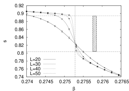
Figure 3: Entropy density in the vicinity of the phase transition. The height of the bar on the right represents the entropy gap $\Delta s$. The horizontal lines are $s^{+}$ and $s^{-}$ and the vertical line is $\beta^{2}_{c}$.

To determine the endpoints of the entropy and energy on the disordered and ordered side of the transition, we introduce a second definition of inverse pseudo-transition temperatures, $\beta^{2}_{pt}(L)$, which differ from the equal heights definition in crucial details. We adjust the weights of the double peak histograms so that

$$e_{L}(\beta^{2}_{pt})=\frac{1}{2}\left[e_{L}^{+}(\beta^{2}_{pt})+e_{L}^{-}(\beta^{2}_{pt})\right]$$ (21)

holds, where the central energy density $e_{L}(\beta^{2}_{pt})$ is the expectation value at $\beta^{2}_{pt}(L)$ and $e_{L}^{\pm}(\beta^{2}_{pt})$ are the locations of the maxima of the double peak histogram at $\beta^{2}_{pt}(L)$, $e_{L}^{+}$ on the disordered and $e_{L}^{-}$ on the ordered side of the transition. The idea behind this construction is to ensure that the energy endpoints (4) are positioned symmetrically about the central energy density:

$$e_{L}^{\pm}=e_{L}(\beta^{2}_{c})\pm\frac{1}{2}\,\Delta e_{L}\,.$$ (22)

In the following we call this procedure equal distances reweighting. Using (5) and (6) one finds that

$$s_{L}^{\pm}=s_{L}(\beta^{2}_{c})\pm\frac{1}{2}\,\Delta s_{L}$$ (23)

holds as well.

Figure 4: Histograms of the energy density reweighted to equal distances on various lattices.

Table 3: Second inverse pseudo-transition temperature, central energy and and entropy densities on $L^{3}$ lattices.

$L$	$\beta^{2}_{pt}$	$e_{L}(\beta^{2}_{pt})$	$s_{L}(\beta^{2}_{pt})$	$f_{L}(\beta^{2}_{pt})$
30	0.275166 (13)	$-1.336~{}$ (14)	0.8522 (37)	$-4.43275~{}$ (14)
40	0.2752369 (52)	$-1.345~{}$ (11)	0.8497 (29)	$-4.431840$ (62)
50	0.2752508 (22)	$-1.3444$ (51)	0.8498 (14)	$-4.431652$ (26)

The histograms reweighted to equal distances are shown in Fig. 4 and the corresponding $\beta^{2}_{pt}(L)$ are collected in Table 3. For the $L=20$ histogram of the figure $\beta=0.275311$ is used just to illustrate that the double peak disappears before condition (21) gets fulfilled. This is the reason why there are no $L=20$ values in the table. Fitting the $\beta^{2}_{c}(L)$ values of Table 3 to (13) yields

$$\beta^{2}_{c}=0.2752724\,(44),\,\,\,\,\,b^{2}=-2.61\,(40)$$ (24)

with a goodness of fit $Q=0.21$. The estimates (14) and (24) are at the edge of being consistent ($Q=0.051$ for the Gaussian difference test). Our second estimate for $\beta_{c}$ is less accurate than our first, apparently because the location of the newly defined maxima of the energy probability density is less stable than for the equal heights definition. Also FS corrections to the second estimate are not negligible as those to the first. In absolute numbers the difference is less than 1 in the fifth significant digits, so it does not propagate into the $\beta_{c}$ factor used for the far less accurate latent heat. Still the second definition is needed to enable estimates of $e^{\pm}$ and $s^{\pm}$.

To give a combined estimate of $\beta_{c}$, we average the $\beta^{1}_{c}$ and $\beta^{2}_{c}$ estimates weighted by their inverse variances and keep the error bar procedure of the more accurate $\beta^{1}_{c}$ result to obtain

$$\beta_{c}=0.2752796\,(29)\,.$$ (25)

For comparison, the weighted average of JV97 on lattices $L=10,\,\dots\,,36$ is $\beta_{c}=0.2752825(50)$ and the Gaussian difference test with our value gives $Q=0.62$.

To calculate $\Delta s$ and $\Delta e$ we define jackknife estimators on finite lattices for them:

$$\Delta s_{L}=2\,\sqrt{\frac{C_{\max}(L)}{L^{3}}}\,.$$ (26)

and

$$\Delta e_{L}=\frac{2}{\beta^{2}_{pt}(L)}\,\sqrt{\frac{C_{\max}(L)}{L^{3}}}\ .$$ (27)

Their values will be needed for combination with jackknifed central entropy and energy values, so error bars for $e^{\pm}$ and $s^{\pm}$ can be obtained. Only $L\geq 30$ lattices are used as we have already seen for $a_{2}$ that the smallest lattice spoils the fit. Estimates of the means and their error bars follow in the usual jackknife way. Fitting them with $1/L^{3}$ corrections, the entropy gap is

$$\Delta s=0.09045\,(41)\ .$$ (28)

It is represented by the height of the filled bar on the right of Fig. 3. In the same way we find for the latent heat

$$\Delta e=\frac{\Delta s}{\beta_{c}}=0.3286\,(15)\ .$$ (29)

This value is somewhat larger than $\Delta e=0.32320\,(94)$ of JV97 ($Q=0.002$) and in agreement with $\Delta e=0.3291\,(33)$ of ABV91 where additional data of FMOU90 on lattices up to $L=48$ was taken into account ($Q=0.89$). However, these results depend still beyond the range of one error bar on the order in which the functions are evaluated. Using (9) and (8) to estimate the gaps from $a_{2}$ of Eq. (20), one finds $\Delta s=0.08933\,(38)$ and $\Delta e=0.3245\,(14)$. This $\Delta e$ value is consistent with both results of the previous literature as it is in the middle of them.

The central energy (21), entropy and free energy density values (all defined at $\beta^{2}_{pt}$) are listed in Table 3. From

$$e_{L}(\beta^{2}_{pt})=e(\beta^{2}_{c})+\frac{c}{L^{3}},$$ (30)

we find the infinite volume extrapolation

$$e(\beta^{2}_{c})=-1.3470\,(74)\,,\qquad Q=0.82\,.$$ (31)

Similarly we determine

$$s(\beta^{2}_{c})=0.8491\,(21)\,,\qquad Q=0.82\,,$$ (32)

and the corresponding (5) free energy density

$$f(\beta^{2}_{c})=-4.431364\,(50)\,,\qquad Q=0.18\,.$$ (33)

The statistical errors of $f_{L}(\beta^{2}_{pt})$ are quite small due to correlations between $e_{L}(\beta^{2}_{pt})$ and $s_{L}(\beta^{2}_{pt})$.

Table 4: Results for $e^{\pm}_{L}$ (22) and $s^{\pm}_{L}$ (23).

$L$	$e^{+}_{L}$	$e^{-}_{L}$	$s^{+}_{L}$	$s^{-}_{L}$
30	$-1.161~{}$ (13)	$-1.511~{}$ (15)	0.9003 (36)	0.8041 (39)
40	$-1.177~{}$ (10)	$-1.513~{}$ (12)	0.8958 (28)	0.8035 (31)
50	$-1.1777$ (50)	$-1.5111$ (53)	0.8957 (14)	0.8039 (15)

From (22) and (23) we find finite lattice estimators $e_{L}^{\pm}$ and $s_{L}^{\pm}$, which are collected in Table 4. Fits with $1/L^{3}$ corrections give:

$$e^{+} = -1.1826\,(73)\,,\qquad Q=0.74\,,$$ (34)

$$e^{-} = -1.5112\,(79)\,,\qquad Q=0.88\,,$$ (35)

$$s^{+} = 0.8943\,(21)\,,~{}~{}\qquad Q=0.73\,,$$ (36)

$$s^{-} = 0.8038\,(22)\,,~{}~{}\qquad Q=0.90\,.$$ (37)

The values of $s^{+}$ and $s^{-}$ are shown in Figs. 2 and 3 as horizontal lines. The vertical line in Fig. 3 represents the inverse transition temperature (24).

IV Summary and Conclusions

The main result of this work is the entropy density with proper normalization, shown in Fig. 2, where $s_{0}=\ln 3$. The transition region is enlarged in Fig. 3. The values of the entropy density $s^{+}$ (36) on the disordered and $s^{-}$ (37) on the ordered side of the transition in % of $s_{0}$ are, respectively, 82% and 73%. Thus, there are 3 states per site at infinite temperature and effectively 2.45 states on the high- and 2.24 states on the low-temperature side of the phase transition. Our corresponding $e^{\pm}$ estimates are given in Eqs. (34) and (35).

Other results are $\beta_{c}$ (25), the free energy density at the critical point (33), the entropy gap (28), the latent heat (29) and the interface tension (19). It is notable that the inclusion of capillary waves enhances the estimate of the interface tension by more than 10%.

- (1) B. Svetitsky and L.G. Yaffe, Nucl. Phys. B 210, 443 (1982).
- (2) R.V. Gavai, F. Karsch, and B. Petersson, Nucl. Phys. B 322, 738 (1989).
- (3) M. Fukugita, H. Mino, M. Okawa, and A. Ukawa, J. Stat. Phys. 59, 1397 (1990).
- (4) N. Alves, B.A. Berg and R. Villanova, Phys. Rev. B 43, 5846 (1991).
- (5) M. Schmidt, Z. Phys. B95, 327 (1994).
- (6) W. Janke and R. Villanova, Nucl. Phys. B 489, 679 (1997).
- (7) F. Karsch and S. Stickan, Phys. Lett. B 488, 319 (2000).
- (8) B.A. Berg and T. Neuhaus, Phys. Rev. Lett. 68, 9 (1992).
- (9) B.A. Berg, Markov Chain Monte Carlo Simulations and Their Statistical Analysis (World Scientific, Singapore, 2004).
- (10) K. Binder, Phys. Rev. A 25, 1699 (1982).
- (11) M.S.S. Challa, D.P. Landau, and K. Binder, Phys. Rev. B 34, 1841 (1986).
- (12) E. Brézin and J. Zinn-Justin, Nucl. Phys. B 257, 867 (1985).
- (13) M.P. Gelfand and M.E. Fisher, Physica A 166, 1 (1990).
- (14) J.J. Moris, J. Stat. Phys. 69, 539 (1991).
- (15) A. Billoire, T. Neuhaus and B.A. Berg, Nucl. Phys. B 413, 795 (1994).
- (16) This error bar should not be reduced when combining and , because they rely on the same simulations.