ROM2F/2007-03

MS-TP-07-1

CERN-PH-TH/2007-018

MKPH-T-07-03

TRINLAT-07/03

February 2007

Flavour symmetry restoration and

kaon weak matrix elements in quenched twisted mass QCD

P. Dimopoulos^a, J. Heitger^b, F. Palombi^c, C. Pena^d, S. Sint^e and A. Vladikas^a

^a INFN, Sezione di Roma II

and Dipartimento di Fisica, Università di Roma “Tor Vergata”

Via della Ricerca Scientifica 1, I-00133 Rome, Italy

^b Westfälische Wilhelms-Universität Münster, Institut für Theoretische Physik

Wilhelm-Klemm-Strasse 9, D-48149 Münster, Germany

^c Johannes Gutenberg Universität, Institut für Kernphysik

Johann Joachim Becher-Weg 45, D-55099 Mainz, Germany

^d CERN, Physics Department, TH Division, CH-1211 Geneva, Switzerland

^e School of Mathematics, Trinity College, Dublin 2, Ireland

 Abstract We simulate two variants of quenched twisted mass QCD (tmQCD), with degenerate Wilson quarks of masses equal to or heavier than half the strange quark mass. We use Ward identities in order to measure the twist angles of the theory and thus check the quality of the tuning of mass parameters to a physics condition which stays constant as the lattice spacing is varied. Flavour symmetry breaking in tmQCD is studied in a framework of two fully twisted and two standard Wilson quark flavours, tuned to be degenerate in the continuum. Comparing pseudoscalar masses, obtained from connected quark diagrams made of tmQCD and/or standard Wilson quark propagators, we confirm that flavour symmetry breaking effects, which are at most $5\%$, decrease as we approach the continuum limit. We also compute the pseudoscalar decay constant in the continuum limit, with reduced systematics. As a consequence of improved tuning of the mass parameters at $\beta=6.1$, we reanalyse our previous $B_{K}$ results. Our main phenomenological findings are $r_{0}f_{K}~{}=~{}0.421(7)$ and $\hat{B}_{K}=0.735(71)$.  

1 Introduction

$B_{K}$, the bag parameter of neutral $K$-meson oscillations, has been computed with several discretizations of lattice fermions. Until recently, the quenched Wilson fermion results of $B_{K}$ were the least accurate, due to a limited control of those systematic sources of error, which arise form the lack of chiral symmetry in the regularization. This trend has been reversed in ref. [1], thanks to the implementation of twisted Wilson fermions [2]. The simulations of ref. [1], besides introducing some novelties in the computation of $B_{K}$ (twisted mass QCD (tmQCD) regularization, Schrödinger functional renormalization and RG running) have also been extensive from the computational point of view. In particular two tmQCD variants of the fermion action have been implemented (with twist angles $\pi/2$ and $\pi/4$) at several inverse gauge couplings $\beta$. Such a large collection of data enables us to address, in the present work, several other issues related to the tmQCD formalism, in the region of strange quarks. Clearly, the fact that we work in the quenched approximation is a limitation of the scope of the present work. In sect. 2 we present the details of our formalism. In our first tmQCD variant we introduce two twisted flavours, with twist angle $\pi/2$, and two standard (untwisted) flavours. In the second variant we only have two twisted flavours with twist angle $\pi/4$. The tmQCD lattice action is $O(a)$ improved. All dimension-3 operators (currents, scalar and pseudoscalar densities) are improved by introducing $O(a)$ Symanzik counterterms. This is essential to $O(a)$ improvement in the $\pi/4$ case and to those quantities of the $\pi/2$ case which are not exclusively composed of fully twisted quarks. No improvement of the four-fermion operators is attempted. In sect. 3, we first of all examine the quality of the tuning of the mass parameters, fixed so as to ensure that the twist angle is equal to a target reference value (in our case $\pi/2$ or $\pi/4$). This, together with the requirement that all quark masses be degenerate and phenomenological quantities be measured at a reference pseudoscalar meson mass, constitute our constant physics requirement. It has to be maintained as we increase the theory’s UV cutoff (i.e. approach the continuum limit). The twist angle is then measured with the aid of Ward identities and compared to its target reference value, used in the mass parameter tuning. We see that $O(a^{2})$ cutoff effects are responsible for statistically significant discrepancies, which are nevertheless only a few percent. In sect. 4, we measure the pseudoscalar masses and decay constants in both $\pi/2$ and $\pi/4$ setups. In the former case we are also able to monitor flavour breaking effects, arising from the twisted mass term in the lattice action. This we do by comparing the pseudoscalar masses and decay constants for mesons composed exclusively of twisted or untwisted valence quarks, as well as those made of one twisted and one untwisted quark. For the pseudoscalar masses, we find that statistically significant effects, which are nevertheless only a few percent at the coarsest lattices, disappear as the lattice spacing is decreased. Thus flavour symmetry appears to be restored in the continuum limit. Our best results for the $K$-meson decay constant are based on a tmQCD Ward identity. They are free of the usual systematic uncertainties arising from current normalizations and improvement (i.e. ambiguities in the values of $Z_{\rm\scriptscriptstyle A}$, $Z_{\rm\scriptscriptstyle V}$ and $c_{\rm\scriptscriptstyle A}$). Extrapolating $\pi/2$ and $\pi/4$ results to a common continuum limit gives a result in full agreement with earlier estimates. The more detailed analysis concerning the accuracy of the tuning of quark masses and twist angles, presented here, was performed after the publication of ref. [1]. The quality of the tuning was found to be satisfactory in all cases, save for the simulations at $\beta=6.1$, mainly in the $\pi/4$ case. This is signalled e.g. by relatively large differences between the value of the target twist angle, set to $\pi/2$ or $\pi/4$ through the tuning of the bare (subtracted) mass parameters, and the value obtained by computing the twist angle with the PCAC quark mass instead of the subtracted quark mass. The reason for this behaviour has been traced back to the value of $\kappa_{\rm cr}$ taken as input from the literature. Indeed, for an accurate determination of $\kappa_{\rm cr}$ it is crucial to fix its $O(a^{2})$ ambiguities by following a constant physics condition in the approach to the continuum limit. Instead, the value of $\kappa_{\rm cr}(\beta=6.1)$ quoted in [3] comes from an interpolation of data obtained from a constant physics condition at other values of $\beta$. While the effect of relaxing the constant physics requirement was found to be negligible for the data of [3], its impact on the tuning of twist angles is large. This is discussed in detail in Appendix A. The $\beta=6.1$ critical point has been hence determined afresh, and $\beta=6.1$ simulations with new mass parameters have been performed. Thus all results in the present work are generated from the datasets of ref. [1], except for those at $\beta=6.1$, which are completely new. The new $B_{K}(\beta=6.1)$ results can be found in sect. 5. They induce a reanalysis of the continuum limit extrapolation of this quantity. Also in sect. 5, we collect our detailed results of the kaon-to-pion four-fermion operator matrix elements, involved in the $\Delta I=1/2$ rule. Strictly speaking, these results are not physical, as they refer to four degenerate quarks, with masses close or above half the strange quark mass. They have been used, however, in ref. [4] in order to obtain the relevant four-fermion operator renormalization with Neuberger fermions, through a matching procedure of RGI matrix elements computed from both tmQCD and Neuberger regularizations. For the sake of legibility, all tables containing our results have been gathered in Appendix B.

2 General tmQCD formalism

Twisted mass QCD has been designed to eliminate exceptional configurations in (partially) quenched lattice simulations with light Wilson quarks [2]. In its original formulation, it describes a mass-degenerate isospin doublet $\psi$ of Wilson quarks for which, besides the standard mass term, a so-called twisted mass term $i\mu_{\rm q}\bar{\psi}\gamma_{5}\tau^{3}\psi$ is introduced. The properties of tmQCD have been studied in detail in [2], where, in particular, its equivalence to standard two-flavour QCD has been established. We discuss here the main characteristics of this formulation, extended to more flavours, in ways analogous to those discussed in [8] and [1]. It is convenient to formalize our variant of tmQCD in terms of a twisted and an untwisted isospin doublet, denoted as $\bar{\psi}_{\rm tw}=(\bar{\psi}_{1},\bar{\psi}_{2})$ and $\bar{\psi}_{\rm w}=(\bar{\psi}_{3},\bar{\psi}_{4})$ respectively. All flavours will eventually be tuned to be degenerate. The twisted (untwisted) isospin doublet is regularized in the standard tmQCD-Wilson (plain Wilson) fashion:

$$S_{F}=a^{4}\sum_{x}\,\,[ \ {\bar{\psi}_{\rm tw}}(x)(D_{\rm w}+m_{0,{\rm tw}}+i\gamma_{5}\tau^{3}\mu_{0,{\rm tw}})\psi_{\rm tw}(x)$$

$$+\bar{\psi}_{\rm w}(x)(D_{\rm w}+m_{0,{\rm w}})\psi_{\rm w}(x)\ ]\ ,$$ (2.1)

where $D_{\rm w}$ is the standard Dirac-Wilson fermion matrix (with a Clover term) and $\tau^{3}$ the Pauli isospin matrix. In this work, the Wilson plaquette action is the regularization of the pure gauge sector of the theory. For the rest of the notation, relating tmQCD to standard QCD (concerning field rotations, mass transformations etc.) see [1]. Here, what we are mostly interested in are the expressions for the renormalized quark mass in the twisted quark sector, given by the combination of standard and twisted mass parameters

$$M_{\rm R,tw}=\sqrt{m_{\rm R,tw}^{2}+\mu_{\rm R,tw}^{2}}\ ,$$ (2.2)

and the twist angle, defined in terms of renormalized masses as

$$\tan\alpha=\dfrac{\mu_{{\rm R},{\rm tw}}}{m_{{\rm R},{\rm tw}}}\,\,.$$ (2.3)

Also standard is the relation between renormalized and bare quark masses: the subtracted (unrenormalized) quark mass for Wilson fermions in denoted by $am_{\rm q}=1/(2\kappa)-1/(2\kappa_{\rm cr})$, $\kappa$ being the hopping parameter ($2\kappa=[am_{0}+4]^{-1}$). Whenever we need to identify the quark doublet $f$ (with $f={\rm tw},{\rm w}$), we will denote the corresponding quantities by $am_{{\rm q},f}$ and $\kappa_{f}$. In a Symanzik $O(a)$ improved framework, the renormalized quenched quark masses for the untwisted flavours are given by

$$m_{{\rm R},{\rm w}}=Z_{\rm m}[m_{{\rm q},{\rm w}}(1+b_{\rm m}am_{{\rm q},{\rm w}})]\ ,$$ (2.4)

while the twisted quark masses renormalize as follows:

$$m_{{\rm R},{\rm tw}} = Z_{\rm m}[m_{{\rm q},{\rm tw}}(1+b_{\rm m}am_{{\rm q},{\rm tw}})+{\tilde{b}}_{\rm m}a\mu_{0,{\rm tw}}^{2}]\ ,$$ (2.5)

$$\mu_{{\rm R},{\rm tw}} = Z_{\rm\scriptscriptstyle P}^{-1}\mu_{0,{\rm tw}}(1+b_{\mu}am_{{\rm q},{\rm tw}})\ .$$ (2.6)

In terms of the last two expressions, the twist angle may be expressed as [9]

$$\tan(\alpha)=\dfrac{a\mu_{0,{\rm tw}}[1+(b_{\mu}-b_{\rm m})am_{{\rm q},{\rm tw}}]}{Z_{\rm\scriptscriptstyle P}Z_{\rm m}[am_{{\rm q},{\rm tw}}+{\tilde{b}}_{\rm m}(a\mu_{0,{\rm tw}})^{2}]}\,\,.$$ (2.7)

We now discuss an alternative expression for the twist angle, obtained in terms of Ward identities in [9]. For the twisted sector of our theory, the PCAC and PCVC Ward identities read

$$\tilde{\partial}_{\nu}(A_{\rm R})_{\nu,12} = 2m_{\rm R}(P_{\rm R})_{12}\ ,$$ (2.8)

$$\tilde{\partial}_{\nu}(V_{\rm R})_{\nu,12} = 2i\mu_{\rm R}(P_{\rm R})_{12}\ ,$$ (2.9)

and they are valid up to $O(a^{2})$ for the Symanzik-improved operators [9]

$$(P_{\rm R})_{12} = Z_{\rm\scriptscriptstyle P}[1+b_{\rm\scriptscriptstyle P}am_{{\rm q},{\rm tw}}]P_{12}\ ,$$ (2.10)

$$(A_{\rm R})_{\nu,12} = Z_{\rm\scriptscriptstyle A}[1+b_{\rm\scriptscriptstyle A}am_{{\rm q},{\rm tw}}][A_{\nu,12}+ac_{\rm\scriptscriptstyle A}\tilde{\partial}_{\nu}P_{12}-i{\tilde{b}}_{\rm\scriptscriptstyle A}a\mu_{0,{\rm tw}}V_{\nu,12}]\ ,$$ (2.11)

$$(V_{\rm R})_{\nu,12} = Z_{\rm\scriptscriptstyle V}[1+b_{\rm\scriptscriptstyle V}am_{{\rm q},{\rm tw}}][V_{\nu,12}+ac_{\rm\scriptscriptstyle V}\tilde{\partial}_{\rho}T_{\nu\rho,12}-i{\tilde{b}}_{\rm\scriptscriptstyle V}a\mu_{0,{\rm tw}}A_{\nu,12}]\ ,$$ (2.12)

where $\tilde{\partial}_{\nu}$ denotes the lattice symmetrized derivative and the operator subscripts $1,2$ indicate quark flavours. By combining expressions (2.8) - (2.12) with the standard definition of the PCAC bare quark mass [10],

$$\tilde{\partial}_{\nu}[A_{\nu,12}+c_{\rm\scriptscriptstyle A}a\tilde{\partial}_{\nu}P_{12}]=2m_{\rm tw}P_{12}\ ,$$ (2.13)

the renormalized quark mass is computed as

$$m_{{\rm R},{\rm tw}}=\dfrac{Z_{\rm\scriptscriptstyle A}[1+b_{\rm\scriptscriptstyle A}am_{{\rm q},{\rm tw}}]}{Z_{\rm\scriptscriptstyle P}[1+b_{\rm\scriptscriptstyle P}am_{{\rm q},{\rm tw}}]}\Big{[}m_{\rm tw}+a\mu_{0,{\rm tw}}^{2}{\tilde{b}}_{\rm\scriptscriptstyle A}Z_{\rm\scriptscriptstyle V}^{-1}\Big{]}\ .$$ (2.14)

Finally, the PCAC expression for the twist angle, in terms of the above, is [9]

$$\tan(\alpha)=\dfrac{a\mu_{0,{\rm tw}}[1+(b_{\mu}+b_{\rm\scriptscriptstyle P}-b_{\rm\scriptscriptstyle A})am_{{\rm q},{\rm tw}}]}{Z_{\rm\scriptscriptstyle A}[am_{\rm tw}+\tilde{b}_{\rm\scriptscriptstyle A}(a\mu_{0,{\rm tw}})^{2}Z_{\rm\scriptscriptstyle V}^{-1}]}\,\,.$$ (2.15)

Yet another variant of the twist angle is obtained by expressing $\mu_{{\rm R},{\rm tw}}$ in terms of the PCVC Ward identity. We define the PCVC bare twisted mass from

$$\tilde{\partial}_{\nu}V_{\nu,12}=2i\mu_{\rm tw}P_{12}\ ,$$ (2.16)

and, using expressions (2.8) - (2.12), obtain for the renormalized twisted mass

$$\mu_{{\rm R},{\rm tw}}=\dfrac{Z_{\rm\scriptscriptstyle V}[1+b_{\rm\scriptscriptstyle V}am_{{\rm q},{\rm tw}}]}{Z_{\rm\scriptscriptstyle P}[1+b_{\rm\scriptscriptstyle P}am_{{\rm q},{\rm tw}}]}\Big{[}1-am_{\rm tw}Z_{\rm\scriptscriptstyle V}{\tilde{b}}_{\rm\scriptscriptstyle V}\Big{]}\mu_{\rm tw}\ .$$ (2.17)

The PCVC expression for the twist angle, in terms of the above, is

$$\tan(\alpha)=\dfrac{Z_{\rm\scriptscriptstyle V}a\mu_{\rm tw}[1+(b_{\rm\scriptscriptstyle V}-b_{\rm\scriptscriptstyle A}-Z_{\rm\scriptscriptstyle V}\tilde{b}_{\rm\scriptscriptstyle V})am_{{\rm q},{\rm tw}}]}{Z_{\rm\scriptscriptstyle A}[am_{\rm tw}+\tilde{b}_{\rm\scriptscriptstyle A}(a\mu_{\rm tw})^{2}Z_{\rm\scriptscriptstyle V}^{-1}]}\,\,.$$ (2.18)

In the present work, expression (2.7) is used for tuning the bare mass parameters $\mu_{0,{\rm tw}}$ and $\kappa_{\rm tw}$, so as to fix the theory to a specific twist angle. One also needs the value of $\kappa_{\rm cr}$ for the determination of $am_{{\rm q},l}$. This is known from previous Schrödinger functional computations, based on the Clover-improved theory with Wilson (untwisted) quarks. Once the bare parameters are thus fixed to satisfy Eq. (2.7), one may use Eq. (2.15) and Eq. (2.18) in order to obtain independent estimates of the twist angle, which differ from the target value by $O(a^{2})$ discretization effects. This provides a measure of the systematic uncertainties related to the tuning of the twist angle. Finally, we specify the twist angles, following the two cases of [1]. In the first case, known as fully twisted theory, the bare parameters of the twisted quark doublet are tuned so as to ensure that $\alpha=\pi/2$. This amounts to tuning Eq. (2.5) so that $m_{{\rm R},{\rm tw}}=0$. The untwisted doublet is also tuned (through an opportune choice of $\kappa_{\rm w}$), so that $m_{{\rm R},{\rm w}}=\mu_{{\rm R},{\rm tw}}$ up to $O(a^{2})$; cf. Eqs.(2.4) and (2.6). In the second case we switch off the untwisted doublet, keeping just two twisted flavours; the twist angle is set to $\alpha=\pi/4$. This amounts to tuning Eqs.(2.5) and (2.6) so as to have $m_{{\rm R},{\rm tw}}=\mu_{{\rm R},{\rm tw}}$. The detailed expressions used for these tunings may be read off from ref. [1]. In order to make contact with the physical results we will be presenting, we now identify the four generic quark fields $\psi_{k}$ ($k=1,\cdots,4$) with physical (if degenerate) flavours. There is a different identification according to the problem in hand. When we discuss pseudoscalar masses, decay constants and $B_{K}$, in the $\pi/2$ case we identify the twisted doublet with $\bar{\psi}_{\rm tw}=(\bar{u},\bar{d})$ and the untwisted one with $\bar{\psi}_{\rm w}=(\bar{s},\bar{c})$. The same quantities in the $\pi/4$ case are addressed in terms of a single twisted doublet of a strange and a down quark; i.e. $\bar{\psi}_{\rm tw}=(\bar{s},\bar{d})$. As our simulations are quenched and mass degenerate, this is sufficient to model two valence quarks. In this way we make full contact with the notation of the earlier tmQCD simulations of ref. [1]. For the results related to $\Delta S=1$ four-fermion operators, the physical flavour identification is more complicated. The reader is referred directly to ref. [4], where the issue has been addressed in detail.

3 Cutoff effects of the twist angle

We now turn to the determination of the twist angle from PCAC and PCVC relations. The simulation parameters are gathered in Table 1 for the $\pi/2$ theory and in Table 2 for the $\pi/4$ one. The data are those of ref. [1], except at $\beta=6.1$. As mentioned in the introduction, the run had to be repeated at this coupling, for reasons which will be discussed in detail below. The physical regime targeted in the runs of ref. [1] is that of the $K$-meson, composed of two degenerate valence quarks. As detailed in that work, in practice this means that the choice of quark masses is such that the $K$-meson in the $\pi/2$ theory is computed in the range $640$–$830~{}{\rm MeV}$ and extrapolated to the physical point at 495 MeV (i.e. $r_{0}M^{\rm phys}_{K}=1.2544$). In the $\pi/4$ theory we are instead able to simulate with quarks corresponding to a physical kaon of about 495 MeV. The only exception is the $\beta=6.45$ case, in which extrapolations from higher mass values were the only option, as simulations with quarks corresponding to a physical kaon require prohibitively large lattice sizes. As the present work is based on the same runs, the same physical point for all four flavours is targeted here. Following the discussion of sect. 2, the bare mass parameters (i.e. standard hopping parameter(s) and twisted mass $\mu_{0,{\rm tw}}$) are tuned at each $\beta$ value so as to keep the quarks degenerate and the twist angle fixed at $\alpha=\pi/2,\pi/4$. The $\kappa_{\rm cr}$ estimates used in the bare parameter calibration are taken over from the literature; see Table 3. Those of ref. [12], as well as the one provided to us by the ZeRo Collaboration, are the result of a direct computation of the PCAC Ward identity at the corresponding bare coupling, using $O(a)$ improved (untwisted) Wilson fermions, whereas the estimates from ref. [3] are the result of an interpolation in $\beta$ of the data of ref. [12]. We will see that this $\kappa_{\rm cr}$ estimate at $\beta=6.1$ results in poor tuning of the bare tmQCD parameters. Thus, following the procedure described in ref. [12], we have recomputed $\kappa_{\rm cr}$ at $\beta=6.1$, finding a different value. This has been done by an independent run, performed at lattice volume $L/a=16$, $T/L=2$ and four PCAC quark mass values in a range $0.025\lesssim am_{\rm av}\lesssim 0.05$, similar to that of ref. [12] (where $m_{\rm av}$ is defined). Our $\kappa_{\rm cr}$ result is obtained by linear exrapolation in the PCAC quark masses, ensuring that our systematics resemble those of ref. [12]. All observables computed in this work are obtained from the large time asymptotic limit of operator correlation functions with Schrödinger functional (SF) boundary conditions. The notation is standard, following closely that adopted in e.g. [1]. For instance, $f_{{\rm\scriptscriptstyle A},12}$ denotes the Schrödinger functional correlation with a fermionic operator $A_{0,12}$ in the bulk and a time-boundary pseudoscalar operator $\bar{\zeta}_{2}\gamma_{5}\zeta_{1}$ at $x=0$. All such correlation functions are properly (anti)symmetrized in time, when used to extract quark masses, effective pseudoscalar masses and decay constants. The bare PCAC and PCVC quark masses of Eqs. (2.13) and (2.16) are obtained from the ratios

$$R_{m_{\rm tw}} = \dfrac{\tilde{\partial}_{0}[f_{{\rm\scriptscriptstyle A},12}(x_{0})+c_{\rm\scriptscriptstyle A}a\tilde{\partial}_{0}f_{{\rm\scriptscriptstyle P},12}(x_{0})]}{2f_{{\rm\scriptscriptstyle P},12}(x_{0})}\ ,$$ (3.19)

$$R_{\mu_{\rm tw}} = -i\dfrac{\tilde{\partial}_{0}f_{{\rm\scriptscriptstyle V},12}(x_{0})}{2f_{{\rm\scriptscriptstyle P},12}(x_{0})}\,\,.$$ (3.20)

From these and Eqs. (2.14), (2.17) we compute the renormalized masses $am_{{\rm R},{\rm tw}}$ and $a\mu_{{\rm R},{\rm tw}}$; from Eqs. (2.15), (2.18) we compute $\cot(\alpha)$. These results are reported in Table 4. The errors are statistical; we have checked that systematic errors due to the uncertainties of $\kappa_{\rm cr}$, the (re)normalization parameters and the improvement coefficients are an order of magnitude smaller than statistical ones. Let us comment on our $\pi/2$ results first. The two $a\mu_{{\rm R},{\rm tw}}$ values (computed from Eq. (2.6) and Eq. (2.17)) have a small but statistically significant discrepancy of less than 3%. Similarly, the result for $am_{{\rm R},{\rm tw}}$ is also statistically different from the target value $am_{{\rm R},{\rm tw}}=0$. The two estimates of the twist angle are only a few percent off the target value $\pi/2$, but the small discrepancies in the $a\mu_{{\rm R},{\rm tw}}$ evaluations do not carry over to the two results for $\cot(\alpha)$, which are nearly always compatible within errors. All observed deviations from the expected target values are attributed to $O(a^{2})$ discretization effects. The $\pi/4$ results display largely the same characteristics, but the mass range spanned by the data (for $\beta<6.45$) is too narrow to discern the details of the dependence of the twist angle upon the quark mass parameters. What we see is that the difference between the two twisted mass estimates $\mu_{{\rm R},{\rm tw}}$ and the standard mass estimate $m_{{\rm R},{\rm tw}}$ is a small but statistically significant effect. The same is true of the two Ward identity estimates of the twist angle, which also differ from the target value $\pi/4$ by a small amount. Finally, we study to which extent the Ward identity estimates of the twist angles approach their target values $\pi/2,\pi/4$ in the continuum limit. We do this by first computing, at fixed $\beta$ value, the quantity $\cot(\alpha)$ at the kaon mass reference scale $M_{K}\equiv M^{\rm phys}_{K}=495$ MeV. This is done by extra/interpolating our data as a function of the pseudoscalar effective mass-squared, expressed in physical units. The result thus obtained is plotted against $\left(a/r_{0}\right)^{2}$ in Fig. 1. A linear extrapolation of $\cot(\alpha)$ to the continuum limit turns out to be unreliable (very large $\chi^{2}/{\rm d.o.f.}$), as the data do not display a monotonic behaviour, with fluctuations which are much larger than their errors. In any case, these fluctuations are only a small effect, reflecting the overall uncertainty of the tuning of the twist angle to a constant target value (which amounts to a condition of constant physics as we approach the continuum limit).

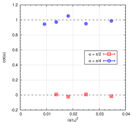
Figure 1: Lattice spacing dependence of $\cot(\alpha)$, computed at the physical kaon mass point, for twist angles $\pi/2$ (circles) and $\pi/4$ (squares). The errors are smaller than the points.

4 Flavour symmetry breaking, meson masses and decay constants

In order to investigate flavour breaking effects, we compare effective pseudoscalar masses, obtained from correlation functions with different combinations of twisted and standard Wilson quark propagators, on our quenched configuration ensemble of tmQCD at $\alpha=\pi/2$. The rationale behind these computations is as follows: we are dealing with a (quenched) lattice QCD model with four degenerate quark flavours, two of which are twisted. The massless continuum theory has an $SU(4)_{\rm L}\otimes SU(4)_{\rm R}$ chiral symmetry with 15 degenerate pseudoscalar Goldstone bosons; with massive fermions we are left with the vector flavour symmetry $SU(4)_{\rm V}$. In the regularized theory, the Wilson term breaks the symmetry induced by axial transformations, even in the absence of quark mass parameters. In twisted mass QCD some of these axial symmetries are interpreted as part of the SU(4) flavour symmetry. With our choice of twisted mass terms one then finds that on the lattice the SU(4) flavour symmetry is reduced to the subgroup $U(1)\otimes U(1)\otimes SU(2)$. Thus, at finite lattice spacing, we expect that the “twisted” charged Goldstone bosons, the “untwisted” ones and the “twisted-untwisted” ones will differ in mass by terms which are like $O(a^{2})$ (recall that we work with a Symanzik-improved action). Based on this approach, we have provided a first summary of our findings on this symmetry breaking in [1]; here we present our full results. The same approach for monitoring such flavour breaking effects has also been implemented (with an action with two $\pi/2$-twisted isospin doublets and no Clover term) in [14]. Both works focus on pseudoscalar masses in the kaon region. For similar results closer to the chiral limit (for a single $\beta$ value), see [15]. It is fairly straightforward to measure these flavour breaking effects, as the corresponding correlation functions involve only connected diagrams. Recall that there is also a flavour breaking effect between the charged and neutral “twisted” pseudoscalar, which is harder to monitor, as the measurement of the neutral pion mass involves disconnected diagrams; see [16] Studying this flavour breaking is beyond the scope of the present work. We have measured pseudoscalar effective masses $aM^{\rm eff}_{ij}(x_{0})$, using suitable time-dependent correlation functions $f_{({\rm\scriptscriptstyle A}_{\rm R})_{ij}}(x_{0})$ (with $i,j$ distinct flavour indices) of the temporal component of the renormalized axial current $(A_{\rm R})_{ij}$

$$aM^{\rm eff}_{ij}(x_{0})=\dfrac{1}{2}\ln\Bigg{[}\dfrac{f_{({\rm\scriptscriptstyle A}_{\rm R})_{ij}}(x_{0}-a)}{f_{({\rm\scriptscriptstyle A}_{\rm R})_{ij}}(x_{0}+a)}\Bigg{]}\,\,.$$ (4.21)

These quantities are suitably (anti)symmetrized in time and averaged over plateaux, as detailed in [1]. In the language of the twisted action Eq. (2) at twist angle $\pi/2$, the corresponding lattice correlation functions to be used in Eq. (4.21) are:

• $f_{({\rm\scriptscriptstyle A}_{\rm R})_{sd}}(x_{0})\rightarrow\dfrac{1}{\sqrt{2}}[f_{({\rm\scriptscriptstyle A}_{\rm R})_{sd}}(x_{0})-if_{({\rm\scriptscriptstyle V}_{\rm R})_{sd}}(x_{0})]$  ,

• $f_{({\rm\scriptscriptstyle A}_{\rm R})_{ud}}(x_{0})\rightarrow-if_{({\rm\scriptscriptstyle V}_{\rm R})_{ud}}(x_{0})$ ,
  

• $f_{({\rm\scriptscriptstyle A}_{\rm R})_{sc}}(x_{0})\rightarrow f_{({\rm\scriptscriptstyle A}_{\rm R})_{sc}}(x_{0})$ .

The first correlation function is composed of a tmQCD Wilson quark propagator and a standard QCD Wilson quark propagator. From it we derive the “$K$-meson” effective mass, denoted by $aM^{\rm eff}_{sd}$. The second correlation function, composed exclusively of the tmQCD Wilson quark propagator, provides the charged “pion” effective mass $aM^{\rm eff}_{ud}$. Finally, the third correlation function, composed exclusively of the standard QCD Wilson quark propagator, provides the “$D_{s}$-meson” effective mass $aM^{\rm eff}_{sc}$. Since all quark masses are tuned to be degenerate, these are three of the 15 degenerate Goldstone bosons in the continuum limit of our quenched theory. At finite lattice spacing tmQCD induces flavour breaking discretization effects, which are monitored by comparing the values of the three effective masses. The corresponding currents, inserted in the above correlation functions, are the following Symanzik-improved quantities, taken over from Appendix B of [1]:

$$(A_{\rm R})_{\nu,sd} = Z_{\rm\scriptscriptstyle A}[1+\dfrac{1}{2}b_{\rm\scriptscriptstyle A}am_{{\rm q},{\rm w}}][A_{\nu,sd}+ac_{\rm\scriptscriptstyle A}\tilde{\partial}_{\nu}P_{sd}-i\dfrac{1}{2}\tilde{b}_{\rm\scriptscriptstyle A}a\mu_{0,{\rm tw}}V_{\nu,sd}]\ ,$$ (4.22)

$$(V_{\rm R})_{\nu,sd} = Z_{\rm\scriptscriptstyle V}[1+\dfrac{1}{2}b_{\rm\scriptscriptstyle V}am_{{\rm q},{\rm w}}][V_{\nu,sd}-i\dfrac{1}{2}\tilde{b}_{\rm\scriptscriptstyle V}a\mu_{0,{\rm tw}}A_{\nu,sd}]\ ,$$ (4.23)

$$(V_{\rm R})_{\nu,ud} = Z_{\rm\scriptscriptstyle V}[V_{\nu,ud}-i\tilde{b}_{\rm\scriptscriptstyle V}a\mu_{0,{\rm tw}}A_{\nu,ud}]\ ,$$ (4.24)

$$(A_{\rm R})_{\nu,sc} = Z_{\rm\scriptscriptstyle A}[1+b_{\rm\scriptscriptstyle A}am_{{\rm q},{\rm w}}][A_{\nu,sc}+ac_{\rm\scriptscriptstyle A}\tilde{\partial}_{\nu}P_{sc}]\ .$$ (4.25)

Again the $O(a)$ tensor-like counterterm in the above vector currents has been omitted, since it drops out in the correlation functions (it is a sum over space, with periodic boundary conditions, of a discrete spatial divergence). Another estimate of the effective pseudoscalar meson mass, denoted as $a\tilde{M}^{\rm eff}_{ud}$, is obtained by using the correlation $f_{({\rm\scriptscriptstyle P}_{\rm R})_{ud}}$ in Eq. (4.21), with

$$(P_{\rm R})_{ud}=Z_{\rm\scriptscriptstyle P}[1+b_{\rm\scriptscriptstyle P}am_{{\rm q},{\rm tw}}]P_{ud}\ .$$ (4.26)

The results are collected in Table 5. The agreement between $M^{\rm eff}_{ud}$ and $\tilde{M}^{\rm eff}_{ud}$ is excellent. In Fig. 2 the ratio $\left(M_{sd}/M_{sc}\right)^{2}$, plotted against $\left(M_{sd}/M^{\rm phys}_{K}\right)^{2}$ with $M^{\rm phys}_{K}=495$ MeV, is compared to $\left(M_{ud}/M_{sc}\right)^{2}$. Note that the statistical errors of these ratios turn out to be very small, due to the strong correlations between numerator and denominator. We see that at $\beta=6.0$ the two ratios are incompatible; their deviation from unity (which quantifies flavour breaking) is at most a $5\%$ effect. As we approach the continuum limit at $\beta=6.3$, the two ratios become compatible and their deviation from unity reduces to $1-2\%$. Our conclusion is that flavour symmetry breaking effects at the mass ranges we are considering appear to be under control, diminishing fast as the continuum limit is approached. Besides this general conclusion, there are a couple of observations to be made: (i) At $\beta=6.0$ we find that $M_{ud}<M_{sd}$, in agreement to the findings of [14] (see Fig. 13 of that work) ; (ii) at fixed reference mass $(M_{sc}/M^{\rm phys}_{K})^{2}$, these mass ratios do not display a monotonic dependence on $\beta$. This is probably a small cumulative effect of the many systematic uncertainties of the mass tuning procedure. A similar analysis is performed for the pseudoscalar meson decay constants. In the Schrödinger functional framework they are obtained from the axial current correlation functions $f_{{\rm\scriptscriptstyle A}_{\rm R}}$, properly normalized by the boundary-to-boundary correlation function $f_{1}$; see [17] for details. For the tmQCD $\pi/2$ case under investigation, the specific expressions are (in the large time asymptotic regime):

$$F_{sd} \approx {\sqrt{2}}(M^{\rm eff}_{sd}L^{3})^{-1/2}\exp[(x_{0}-T/2)M^{\rm eff}_{sd}]\dfrac{f_{({\rm\scriptscriptstyle A}_{\rm R})sd}(x_{0})-if_{({\rm\scriptscriptstyle V}_{\rm R})sd}(x_{0})}{\sqrt{f_{1,sd}}}\ ,$$ (4.27)

$$F_{ud} \approx 2(M^{\rm eff}_{ud}L^{3})^{-1/2}\exp[(x_{0}-T/2)M^{\rm eff}_{ud}]\dfrac{-if_{({\rm\scriptscriptstyle V}_{\rm R})ud}(x_{0})}{\sqrt{f_{1,ud}}}\ ,$$ (4.28)

$$F_{sc} \approx 2(M^{\rm eff}_{sc}L^{3})^{-1/2}\exp[(x_{0}-T/2)M^{\rm eff}_{sc}]\dfrac{f_{({\rm\scriptscriptstyle A}_{\rm R})sc}(x_{0})}{\sqrt{f_{1,sc}}}\ .$$ (4.29)

The quantities $F_{sd},F_{ud}$ and $F_{sc}$ are obtained from these expressions in a range of $x_{0}\gg 0$ in which the pseudoscalar effective masses have been extracted. A second method for computing $F_{ud}$ is based on the PCVC relation Eq. (2.9), expressed in terms of Schrödinger functional correlation functions:

$$-M_{ud}f_{({\rm\scriptscriptstyle V}_{\rm R})_{ud}}(x_{0})=2i\mu_{{\rm R},{\rm tw}}f_{({\rm\scriptscriptstyle P}_{\rm R})_{ud}}(x_{0})\ .$$ (4.30)

The corresponding decay constant is computed as

$$\tilde{F}_{ud} \approx -4\dfrac{\mu_{{\rm R},{\rm tw}}}{\tilde{M}^{\rm eff}_{ud}}(\tilde{M}^{\rm eff}_{ud}L^{3})^{-1/2}\exp[(x_{0}-T/2)\tilde{M}^{\rm eff}_{ud}]\dfrac{f_{({\rm\scriptscriptstyle P}_{\rm R})ud}(x_{0})}{\sqrt{f_{1,ud}}}\ .$$ (4.31)

The results for the decay constants are collected in Table 6. Note the excellent agreement between the $F_{ud}$ and $\tilde{F}_{ud}$ results, at all $\beta$ values, which is analogous to the agreement between the two $\cot(\alpha)$ computations presented in sect. 3. In Fig. 3 the ratio $F_{sd}/F_{sc}$ is compared to $F_{ud}/F_{sc}$. The situation is qualitatively analogous to that of the mass ratios presented above, in that flavour breaking effects tend to vanish as the continuum limit is approached. These effects range form 13% to 3% with increasing $\beta$; however we show below that these estimates depend heavily on the improvement coefficent of the axial current.

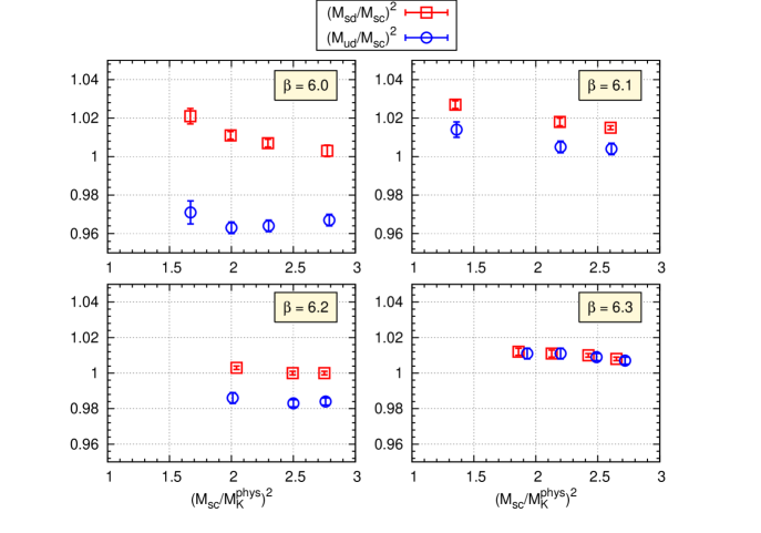
Figure 2: Flavour breaking effects for the quantities $\left(M_{sd}/M_{sc}\right)^{2}$ (squares) and $\left(M_{ud}/M_{sc}\right)^{2}$ (circles), as functions of $\left(M_{sc}/M^{\rm phys}_{K}\right)^{2}$, in the $\pi/2$ theory. In the $\beta=6.3$ plot, the abscissae of the circles are slightly displaced for clarity.

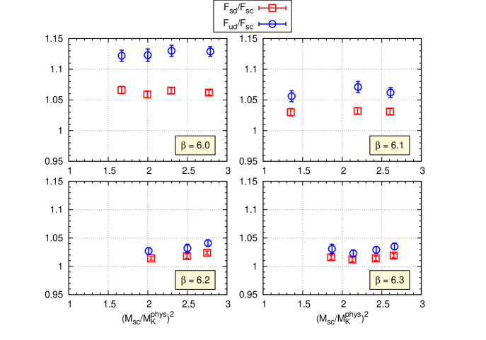
Figure 3: Flavour breaking effects for the quantities $F_{sd}/F_{sc}$ (squares) and $F_{ud}/F_{sc}$ (circles), as functions of $\left(M_{sc}/M^{\rm phys}_{K}\right)^{2}$, in the $\pi/2$ theory.

The above results have been obtained with the normalization constants and improvement coefficients determined in various ALPHA Collaboration publications. In order to monitor their influence on our data, we have repeated the analysis using the LANL Collaboration results for the same quantities (for details, numerical values and references see Appendix A of [1]). The comparison of these results, extrapolated to the physical kaon point, is displayed in Fig. 4. From it we draw the following conclusions:

• The ALPHA and LANL results for each of the decay constants are compatible, the only exceptions being $F_{sc}$ (incompatibility) and $F_{sd}$ (near incompatibility) at $\beta=6.0$. More detailed tests indicate that the main source of incompatibility lies in $c_{\rm\scriptscriptstyle A}(\beta=6.0)$.

• The ALPHA and LANL results for $F_{ud}$ are fully compatible to those for $\tilde{F}_{ud}$. All three are independent from the axial current (cf. Eq. (4.28) and Eq. (4.31)) and thus from $c_{\rm\scriptscriptstyle A}$. Moreover, $\tilde{F}_{ud}$ does not depend on any normalization constants and/or improvement coefficients (cf. Eq. (4.31)).

• Unlike the ALPHA results, at $\beta=6.0$ the three LANL estimates $F_{sc}$, $F_{sd}$ and $F_{ud}$ are fully compatible  and show less scaling violations over the range of simulated couplings. This implies that the $O(a^{2})$ discrepancy shown in Fig. 3 is significantly reduced if $c_{\rm\scriptscriptstyle A}^{\rm LANL}$ is used instead of $c_{\rm\scriptscriptstyle A}^{\rm ALPHA}$. Thus the tmQCD flavour breaking effects under scrutiny, when monitored by decay constant ratios, appear to be obscured by the uncertainty in the $c_{\rm\scriptscriptstyle A}$ determination. The mass ratios of Fig. 2 are a more reliable monitor of tmQCD flavour breaking.

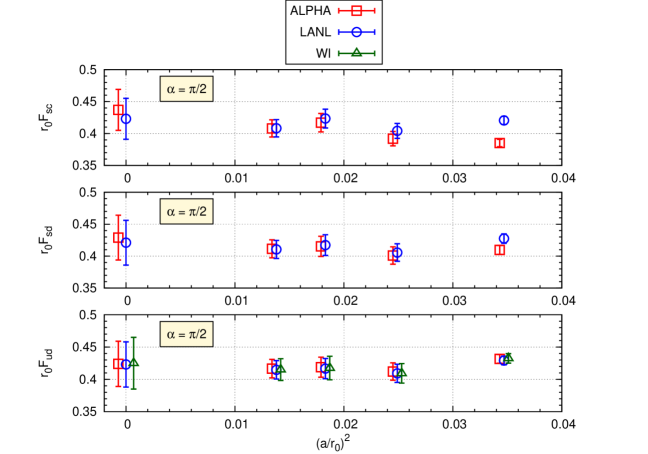
Figure 4: Pseudoscalar meson decay constants, obtained with ALPHA and LANL normalization and improvement coefficients at the physical kaon mass. The twist angle is $\pi/2$. The results for $r_{0}\tilde{F}_{ud}$ (based on a Ward identity) are also shown. The continuum extrapolation (linear in $\left(a/r_{0}\right)^{2}$) is obtained without the $\beta=6.0$ data. The ALPHA and Ward identity abscissae are slightly displaced for clarity.

The continuum limit estimates for the various decay constants of the $\pi/2$ case are obtained by linear extrapolation in $(a/r_{0})^{2}$. Strictly speaking, Symanzik-improved quantities such as the decay constants, contain some improvement coefficients which are only known in perturbation theory (cf. $\tilde{b}_{\rm\scriptscriptstyle A}$ and $\tilde{b}_{\rm\scriptscriptstyle V}$). This means that there are also $O(ag_{0}^{4})$ discretization errors. We have explicitly checked that the influence of the corresponding counterterms is negligible in practice and therefore the dominant discretization error is indeed $O(a^{2})$. From Table 6 we see that our continuum limit results are compatible across all flavour combinations considered. Moreover we note that they do not change substantially if the point of the coarsest lattice ($\beta=6.0$) is removed.  From Fig. 4 we see that the continuum limit extrapolations with ALPHA and LANL data are also compatible. We have also confirmed that this conclusion remains valid if the $\beta=6.0$ data are included in these extrapolations. We now pass to the computation of the kaon masses and decay constants in the $\pi/4$ case. The corresponding lattice correlation function to be used in Eq. (4.21) is:

• $f_{({\rm\scriptscriptstyle A}_{\rm R})_{sd}}(x_{0})\rightarrow\dfrac{1}{\sqrt{2}}[f_{({\rm\scriptscriptstyle A}_{\rm R})_{sd}}(x_{0})-if_{({\rm\scriptscriptstyle V}_{\rm R})_{sd}}(x_{0})]$ ,

where now flavours $s,d$ are both twisted. From it, the estimate $M^{\rm eff}_{sd}$ is obtained. A second estimate $\tilde{M}^{\rm eff}_{sd}$ can also be obtained from the pseudoscalar density correlation function $f_{({\rm\scriptscriptstyle P}_{\rm R})_{sd}}$, with

$$(P_{\rm R})_{sd}=Z_{\rm\scriptscriptstyle P}[1+b_{\rm\scriptscriptstyle P}am_{{\rm q},{\rm tw}}]P_{sd}\ .$$ (4.32)

The decay constant is obtained from the correlation function

$$F_{sd}\approx{\sqrt{2}}(M^{\rm eff}_{sd}L^{3})^{-1/2}\exp[(x_{0}-T/2)M^{\rm eff}_{sd}]\dfrac{f_{({\rm\scriptscriptstyle V}_{\rm R})_{s}d}(x_{0})-if_{({\rm\scriptscriptstyle V}_{\rm R})_{s}d}(x_{0})}{\sqrt{f_{1,sd}}}\ .$$ (4.33)

An alternative derivation is based on the continuum PCAC relation

$$\partial_{\mu}(A_{\rm R})_{\mu,sd}=2M_{\rm R,tw}(P_{\rm R})_{sd}=2{\sqrt{2}}\mu_{{\rm R},{\rm tw}}(P_{\rm R})_{sd}\ .$$ (4.34)

The last equation is derived by taking into consideration that Eq. (2.2) reduces to $Z_{\rm\scriptscriptstyle P}^{-1}{\sqrt{2}}\mu_{0,{\rm tw}}$ for degenerate quark masses $m_{{\rm R},{\rm tw}}=\mu_{{\rm R},{\rm tw}}$. We thus obtain the decay constant estimate

$$\tilde{F}_{sd}\approx-4{\sqrt{2}}\dfrac{\mu_{{\rm R},{\rm tw}}}{M^{\rm eff}_{sd}}(M^{\rm eff}_{sd}L^{3})^{-1/2}\exp[(x_{0}-T/2)M^{\rm eff}_{sd}]\dfrac{f_{({\rm\scriptscriptstyle P}_{\rm R})sd}(x_{0})}{\sqrt{f_{1,sd}}}\ .$$ (4.35)

The results for the decay constants, obtained with ALPHA estimates for the normalization constants and improvement coefficients, are collected in Table 7. In most cases there is again full compatibility between the masses $r_{0}M_{sd}^{\rm eff}$ and $r_{0}\tilde{M}_{sd}^{\rm eff}$, as well as the decay constants $r_{0}F_{ud}$ and $r_{0}\tilde{F}_{ud}$, at all $\beta$ values. The comparison with the LANL results, made at the physical kaon mass, is displayed in Fig. 5. From it we draw the following conclusions:

• The ALPHA and LANL results are compatible, except at $\beta=6.0$.

• Beyond $\beta=6.1$, ALPHA and LANL results for $r_{0}F_{sd}$ are compatible to those for $r_{0}\tilde{F}_{sd}$, the latter being independent of any normalization constants and/or improvement coefficients (cf. Eq. (4.35)). As the ALPHA $r_{0}F_{sd}$ estimate scales like $r_{0}\tilde{F}_{sd}$ for the whole $\beta$ range, the two have almost identical continuum limits.

• Compared to the ALPHA and Ward identity results, the LANL ones display a better scaling behaviour over the whole range of simulated couplings.

The continuum limit extrapolations for the decay constants, linear in $(a/r_{0})^{2}$, are also displayed in Table 7. We see that they are all in good agreement and do not change substantially if the point of the coarsest lattice ($\beta=6.0$) is removed. The same extrapolations (for all $\beta$ values) performed with the LANL data yield $r_{0}F_{sd}=0.404(6)$, which is incompatible to the ALPHA and Ward identity estimates, due to its small error. If however the $\beta=6.0$ point is removed, we obtain the compatible result $r_{0}F_{sd}=0.411(9)$, which is the situation displayed in Fig. 5. The overall conclusion is that the continuum results are remarkably stable for the different flavour combinations, and different tmQCD regularizations (i.e. $\pi/2$ and $\pi/4$ cases). The best result for $F_{K}$ in the continuum limit is obtained with a constrained fit of $\tilde{F}_{ud}$ (for the $\pi/2$ case) and $\tilde{F}_{sd}$ (for the $\pi/4$ case). This choice is dictated by the absence of (re)normalization and improvement coefficients in these quantities, which amounts to the elimination of one source of systematic errors. Our final $F_{K}$ estimate is

$$r_{0}F_{K}=0.421\pm 0.007$$ (4.36)

which agrees nicely with the previous ALPHA result $r_{0}F_{K}=0.415\pm 0.009$ of ref. [18], and the $\chi$LF-Collaboration one $r_{0}F_{K}=0.410\pm 0.011$ of ref. [19].

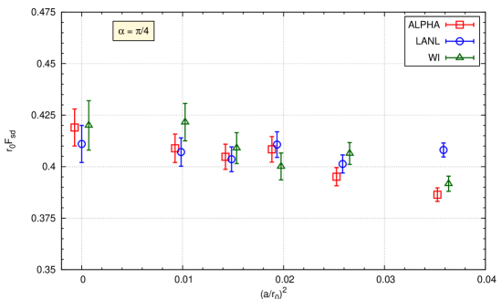
Figure 5: Pseudoscalar meson decay constants, obtained with ALPHA and LANL normalization and improvement coefficients at the physical kaon mass. The twist angle is $\pi/4$. The results for $r_{0}\tilde{F}_{ud}$ (based on a Ward identity) are also shown. The continuum extrapolation (linear in $\left(a/r_{0}\right)^{2}$) is obtained without the $\beta=6.0$ data. The ALPHA and Ward identity ordinates are slightly displaced for clarity.

5 Four-fermion operators

We now pass to the discussion of our tmQCD results concerning the matrix elements of the parity-odd four-fermion operators

$${\cal Q}^{\pm}_{1}=[\bar{\psi}_{1}\gamma_{\mu}\psi_{2}][\bar{\psi}_{3}\gamma_{\mu}\gamma_{5}\psi_{4}]+[\bar{\psi}_{1}\gamma_{\mu}\gamma_{5}\psi_{2}][\bar{\psi}_{3}\gamma_{\mu}\psi_{4}]\pm[2\leftrightarrow 4]$$ (5.37)

between pseudoscalar states. After attributing appropriate physical quark flavours to the four-quark fields $\psi_{k}(k=1,\cdots,4$), we compute the ratios

$${\cal R}_{\pm}=\dfrac{\langle\pi^{+}|{\cal Q}^{\pm}_{1}|K^{+}\rangle}{\langle\pi^{+}|A_{0,ud}|0\rangle\langle 0|A_{0,su}|K^{+}\rangle}\ .$$ (5.38)

These ratios are the core quantities for the calculation of the kaon-to-pion weak matrix elements related to the $\Delta I=1/2$ rule. Note that our computations do not directly provide the physical $K\rightarrow\pi$ matrix elements of interest, as our pseudoscalar mesons (pions and kaons) are degenerate and at best as light as the physical kaon. Nevertheless our results have been used in ref. [4] in order to obtain the renormalization constants of ${\cal Q}_{1}^{\pm}$ with Neuberger fermions. This is achieved through a matching procedure involving the corresponding RGI operators, computed with Wilson fermions. For details on the method and the notation, see ref. [4]. A different relabelling of the operator quarks $\psi_{k}(k=1,\cdots,4$), allows the identification of the matrix element of ${\cal Q}_{1}^{+}$ between pseudoscalar states with $\langle\bar{K}^{0}|Q^{\Delta S=2}|K^{0}\rangle$. Moreover, in the quenched approximation we have the identification $B_{K}=(3/4){\cal R_{+}}$; see refs. [20, 21, 1] for details. Our aim here is twofold: First, we wish to report our $B_{K}$ results at $\beta=6.1$, computed with the new value of $\kappa_{\rm cr}$. Second, we also list the values of ${\cal R_{-}}$ at all couplings; the analysis of ref. [4] was based on these results. As the continuum extrapolation of ${\cal R_{\pm}}$ has also been performed in ref. [4], it needs not to be repeated here. Nevertheless, we will discuss in some detail the continuum extrapolation of $B_{K}$ (which is that of ${\cal R_{+}}$, since $B_{K}=(3/4){\cal R_{+}}$), as this amounts to an update of our older $B_{K}$ result of ref. [1]. This new $B_{K}$ analysis has also been presented in ref. [6].

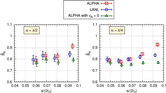
Figure 6: Uncertainties on $\hat{B}_{K}$ related to the $O(a)$ improvement of bilinears. The left panel displays $\pi/2$ data, while the right panel shows $\pi/4$ data.

All computational details are identical to those of ref. [1]. Following that work, we construct three versions of the ratio ${\cal R_{\pm}}$, differing in the structure of the $O(a)$ bilinear counterterm operators in its denominator. The results for ${\cal R_{+}}$ at $\beta=6.1$, are collected in Table 8; the corresponding RGI bag parameter $\hat{B}_{K}$ is shown, for all lattice spacings, in Table 9 and Fig. 6. The determination of $\hat{B}_{K}$ in the continuum limit involves a linear extrapolation in $a$, with the two different regularisations ($\pi/2$ and $\pi/4$) combined in a fit constrained to a common value at zero lattice spacing. It turned out that one of the most relevant sources of cutoff effects is related to the arbitrariness of the denominator $O(a)$ counterterms mentioned above. For instance, using either the values for $Z_{\rm\scriptscriptstyle A},Z_{\rm\scriptscriptstyle V},c_{\rm\scriptscriptstyle A}$ determined by the ALPHA Collaboration or those obtained by the LANL group [22] results in sizeable effects on $B_{K}$ at $\beta=6.0$. At $\beta=6.1$ we also discern discretization effects in the $\pi/4$ case (see Figure 6). This signals the presence of large $O(a^{2})$ ambiguities in $\hat{B}_{K}$ far from the continuum limit. Combined linear+quadratic extrapolation of the data proved to be unreliable, since the curvature of the quadratic term dominates the result also close to the continuum limit. Linear fits, excluding the $\beta=6.0$ data, give

$$\hat{B}_{K} =0.668(45)\,,\qquad {\rm with}\,\,c_{\rm\scriptscriptstyle A}^{\rm ALPHA}\ ;$$ (5.39)

$$\hat{B}_{K} =0.737(51)\,,\qquad {\rm with}\,\,c_{\rm\scriptscriptstyle A}^{\rm LANL}\ ;$$ (5.40)

$$\hat{B}_{K} =0.744(42)\,,\qquad {\rm with}\,\,c_{\rm\scriptscriptstyle A}=0\ ;$$ (5.41)

whereas once also $\beta=6.1$ is excluded we obtain

$$\hat{B}_{K} =0.735(71)\,,\qquad {\rm with}\,\,c_{\rm\scriptscriptstyle A}^{\rm ALPHA}\ ;$$ (5.42)

$$\hat{B}_{K} =0.771(80)\,,\qquad {\rm with}\,\,c_{\rm\scriptscriptstyle A}^{\rm LANL}\ ;$$ (5.43)

$$\hat{B}_{K} =0.780(67)\,,\qquad {\rm with}\,\,c_{\rm\scriptscriptstyle A}=0\ .$$ (5.44)

In the $\pi/2$ case, the error decrease in the extrapolations upon including the $\beta=6.1$ point (for which LANL and ALPHA data are fully compatible), is marginal. For instance, combined linear extrapolations with $c_{\rm\scriptscriptstyle A}^{\rm ALPHA}$, excluding only the $\beta=6.0$ data for $\pi/2$ and those at $\beta=6.0,6.1$ for $\pi/4$, yield $\hat{B}_{K}=0.739(66)$. The above results indicate that the extrapolation of the LANL data is the most stable. In spite of this, the ALPHA data is considered to be the best estimate, on grounds related to the systematic uncertainties in the derivation of $Z_{\rm\scriptscriptstyle A}$, $Z_{\rm\scriptscriptstyle V}$ and $c_{\rm\scriptscriptstyle A}$, as explained at length in ref. [1]. Since the difference between ALPHA and LANL results is only significant at $\beta=6.0$ and $\beta=6.1$, we have conservatively discarded these data points in the continuum extrapolation, illustrated in the left panel of Figure 7. The final results are:

$$\hat{B}_{K} =0.735(71)\,,$$ (5.45)

$$B_{K}^{\overline{\rm MS}}(2~{}{\rm GeV}) =0.534(52)\,.$$ (5.46)

When comparing with the result ($\hat{B}_{K}=0.789(46)$) quoted in [1], we must take into account that the revision of the $\beta=6.1$ data has important consequences for the continuum limit extrapolation. In the analysis of ref. [1] (cf. right panel of Figure 7), good scaling behaviour appeared to set-in rather abruptly at $\beta~{}=~{}6.1$, with continuum limit extrapolation becoming stable only once the $\beta=6.0$ points were discarded. On the contrary, the new $\beta=6.1$ data interpolate in a smoother way those at $\beta=6.0$ and $\beta=6.2$ (cf. left panel of Figure 7). This however, implies a worsening of the scaling behaviour, with continuum limit extrapolation becoming stable only upon discarding our $\beta=6.0$ and $\beta=6.1$ results, as detailed above.

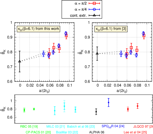
Figure 7: Left: Continuum limit extrapolation of $\hat{B}_{K}$. The $\pi/2$ ordinates have been slightly displaced for clarity. Right: Same as before, but with $\hat{B}_{K}(\beta=6.1)$ from [1]. Bottom: Comparison with other quenched results; different fermion discretizations are as follows (from left to right): [23, 24] domain wall; [25, 26, 27] overlap; [28] Wilson; [29, 30] staggered. The ALPHA point is that of the present work (Wilson tmQCD).

The value of $\hat{B}_{K}$ is shown in the bottom panel of Figure 7 alongside other representative results in quenched QCD found in the literature [23, 24, 25, 26, 27, 28, 29, 30]. Our result is the only quenched result which has simultaneously eliminated the systematic uncertainties related to renormalisation (both at a reference scale and from the point of view of RG running), ultraviolet cutoff dependences, and finite volume effects (within the available accuracy). On the other hand, the control of the mass dependence of $\hat{B}_{K}$ with Wilson fermions is still not as accurate as with e.g. Neuberger or domain wall fermions. The ${\cal R}_{-}$ results for all $\beta$ values are displayed in Tables 10 and 11. The extrapolation of this data to the continuum limit has been presented in ref. [4].

6 Conclusions

In this work we have completed our study of basic kaon weak matrix elements in quenched Wilson tmQCD. Our final value for $F_{K}$ is the best controlled quenched result obtained with Wilson fermions from the point of view of systematic uncertainties. We have also provided a final value for $B_{K}$, with an error that, in our view, reflects faithfully the best accuracy that can be expected for this quantity in the absence of full $O(a)$ improvement. Finally, we have performed a thorough study of flavour breaking in our version of tmQCD, confirming that it does not introduce any uncontrolled systematics in our results. The dominant source of uncertainty left in the quenched approximation (certainly so for $B_{K}$) is related to the lack of full $O(a)$ improvement, which amplifies the error of the continuum limit extrapolation. Thus, if Wilson fermions are to be used in the future in the determination of weak matrix elements, the use of tmQCD variants that embody automatic $O(a)$ improvement [31] may prove essential. Two important aspects of the tmQCD approach are crucial in the context of weak matrix elements: the tuning of mass parameters, in particular of the twist angle, has to be controlled to high precision; and flavour symmetry breaking effects should be reasonably small, as in the present study. In conclusion, the present work demonstrates that, once the tuning of the twisted angle and flavour symmetry breaking are under control, tmQCD may offer a convenient alternative to other discretizations. As we are entering the era of tmQCD simulations with dynamical quarks [32], it will be important to explore these issues in future unquenched studies.

A The effect of an offset in the $\kappa_{\rm cr}$ estimate

In this appendix we present the results for $\cot(\alpha)$, the pseudoscalar effective mass and the decay constant, computed with quark mass parameters tuned with the value of $\kappa_{\rm cr}(\beta=6.1)$ quoted in ref. [3]. As shown in Table 3, this value, obtained by interpolation over a range of $\kappa_{\rm cr}(\beta)$, is roughly only $0.1\%$ off the estimate of the present work, computed directly at $\beta=6.1$. This apparently small offset is nevertheless a discrepancy of 15 standard deviations and has significant consequences in the quantities of interest, which we now examine in some detail. We denote by $\kappa_{\rm cr}$ the value computed on the constant physics condition of ref. [12]; at $\beta=6.1$ this computation has been performed in the present work. The estimate at $\beta=6.1$, obtained through interpolation of data computed at several other gauge couplings [3], is parametrized as $\kappa_{\rm cr}^{\prime}=\kappa_{\rm cr}[1+\delta_{\rm cr}]$. Let us keep track of the effect of this offset in the tuning of the various quark masses, starting with the $\pi/2$ case. The tuning of the hopping parameter $\kappa_{\rm w}$ of the untwisted doublet is done in our simulations by requiring that the pseudoscalar meson made of the two untwisted flavours, has a mass $M^{\rm eff}_{sc}$ equal to a given value, fixed between $640~{}{\rm MeV}$ and $830~{}{\rm MeV}$. This procedure is unaffected by $\kappa_{\rm cr}$, as is the computation of purely untwisted quantities such as $r_{0}F_{sc}$. What is affected by the offset $\delta_{\rm cr}$ is our estimate of the subtracted masses, which now become

$$am_{{\rm q},f}^{\prime}=\dfrac{1}{2\kappa_{f}}-\dfrac{1}{2\kappa_{\rm cr}^{\prime}}=am_{{\rm q},f}+(\delta am_{\rm cr})\,,\qquad(f={\rm tw},{\rm w})\ ,$$ (A.47)

with

$$(\delta am_{\rm cr})\equiv\delta_{\rm cr}/(2\kappa_{\rm cr})+\cdots\,\,,$$ (A.48)

where terms of $O(\delta_{\rm cr}^{2})$ have been dropped. So now Eq. (2.4) becomes

$$am_{{\rm R},{\rm w}}^{\prime}=am_{{\rm R},{\rm w}}+Z_{\rm m}(\delta am_{\rm cr})+\cdots\,\,.$$ (A.49)

where $O(a)$ counterterms are dropped, when multiplied by $\delta am_{\rm cr}$. The requirement of quark mass degeneracy now reads $m_{{\rm R},{\rm w}}^{\prime}=\mu_{{\rm R},{\rm tw}}^{\prime}$; i.e. the offset filters through to the twisted mass, which now becomes

$$a\mu_{{\rm R},{\rm tw}}^{\prime}=a\mu_{{\rm R},{\rm tw}}+Z_{\rm m}(\delta am_{\rm cr})+\cdots\ .$$ (A.50)

This clearly induces an offset $Z_{\rm\scriptscriptstyle P}^{-1}Z_{\rm m}(\delta am_{\rm cr})$ in the tuning of the bare twisted mass parameter, which we therefore denote as $a\mu_{0,{\rm tw}}^{\prime}$. Finally, the hopping parameter of the twisted doublet is tuned to a value $\bar{\kappa}_{\rm tw}$, corresponding to

$$a\bar{m}_{{\rm q},{\rm tw}}^{\prime}=\dfrac{1}{2\bar{\kappa}_{\rm tw}}-\dfrac{1}{2\kappa_{\rm cr}^{\prime}}=a\bar{m}_{{\rm q},{\rm tw}}+(\delta am_{\rm cr})\,\,,$$ (A.51)

by requiring the vanishing of the renormalized light quark mass, which is now written as

$$a\bar{m}_{{\rm R},{\rm tw}}^{\prime}=Z_{\rm m}[a\bar{m}_{{\rm q},{\rm tw}}^{\prime}(1+b_{\rm m}a\bar{m}_{{\rm q},{\rm tw}}^{\prime})+\tilde{b}_{\rm m}(a\mu_{0,\rm tw}^{\prime})^{2}]\,\,.$$ (A.52)

It is important to note that the above quantity is not the true standard quark mass in the twisted sector. Considering that $\kappa_{\rm cr}$ (and not $\kappa_{\rm cr}^{\prime}$) is by definition the reliably estimated critical point, the true renormalized quark mass, for the hopping parameter $\bar{\kappa}_{\rm tw}$, is expressed in terms of $\bar{m}_{{\rm q},{\rm tw}}^{\prime}$ (cf. Eq. (A.51)) as $a\bar{m}_{{\rm q},{\rm tw}}=a\bar{m}_{{\rm q},{\rm}}^{\prime}-(\delta am_{\rm cr})$. It turns out to be non-zero:

$$a\bar{m}_{{\rm R},{\rm tw}}=Z_{\rm m}[a\bar{m}_{{\rm q},{\rm tw}}(1+b_{\rm m}a\bar{m}_{{\rm q},{\rm tw}})+\tilde{b}_{\rm m}(a\mu^{\prime}_{0,\rm tw})^{2}]=-Z_{\rm m}(\delta am_{\rm cr})\ .$$ (A.53)

The second expression has been derived by implementing the vanishing of Eq. (A.52). The bottom line is that we now have a theory characterized by the bare parameters $\kappa_{\rm w},\bar{\kappa}_{\rm tw},\mu_{\rm tw}^{\prime}$ (or, equivalently, $m_{{\rm q},\rm w},\bar{m}_{{\rm q},\rm tw},\mu_{0,\rm tw}^{\prime}$) which correspond to the same heavy quark mass $m_{{\rm R},{\rm w}}$, a small but non-zero light quark mass $\bar{m}_{{\rm R},{\rm tw}}$ and a twisted mass $\mu_{{\rm R},{\rm tw}}^{\prime}$. A twist angle defined through the ratio of mass parameters $a\mu_{{\rm R},{\rm tw}}^{\prime}$ and $a\bar{m}_{{\rm R},{\rm tw}}^{\prime}$, is tautologically equal to $\pi/2$. Instead, the true twist angle of the theory is given by

$$\tan(\bar{\alpha}^{\prime})=\dfrac{a\mu_{{\rm R},{\rm tw}}^{\prime}}{a\bar{m}_{{\rm R},{\rm tw}}}=\dfrac{am_{{\rm R},{\rm w}}^{\prime}}{a\bar{m}_{{\rm R,{\rm tw}}}}=-\dfrac{am_{{\rm q},{\rm w}}}{\delta am_{\rm cr}}+\cdots\ ,$$ (A.54)

which may differ significantly from the target value $\pi/2$. In Table 12, we show the values of $\cot(\alpha)$. It is clear that they are completely incompatible to the target value of $\pi/2$ (and $\pi/4$; see below), on which the mass parameter tuning is based. This is in contrast to the small deviation from the target values of the $\cot(\alpha)$ estimates given in Table 4, which simply reflects the presence of $O(a^{2})$ effects. In Table 13, the results for the various pseudoscalar effective masses and decay constants are presented for the $\pi/2$ case. The quantities $r_{0}M^{\rm eff}_{sc}$ and $r_{0}F_{sc}$ are not reported here, as they are identical to those of Tables 5 and 6. This is because they consist of untwisted flavours, the mass tuning of which is independent of $\kappa_{\rm cr}$. There is a rough check which enables us to “predict” the discrepancy in our results, induced by an offset $\delta\kappa_{\rm cr}$ in the critical point. The standard PCAC dependence of the squared pseudoscalar mass on the average valence quark masses implies that:

$$\left(aM^{\rm eff}_{sc}\right)^{2} \propto 2\,\,am_{{\rm R},{\rm w}}\ ,$$ (A.55)

$$\left(aM^{\rm eff}_{ud}\right)^{2} \propto 2[a\mu_{\rm R,{\rm tw}}+Z_{\rm m}(\delta am_{\rm cr})]\ ,$$ (A.56)

$$\left(aM^{\rm eff}_{sd}\right)^{2} \propto am_{{\rm R},{\rm w}}+a\mu_{{\rm R},{\rm tw}}+Z_{\rm m}(\delta am_{\rm cr})\ .$$ (A.57)

The above expressions have been obtained by keeping track of the offset in the various quark masses (cf. Eqs. (2.2), (A.50) and (A.53)) in the tuning procedure, through straightforward lowest order Taylor expansions in $\delta am_{\rm cr}$. Since, in the absence of offset $\delta am_{\rm cr}$, the quark masses are tuned to satisfy $am_{{\rm R},{\rm w}}=a\mu_{{\rm R},{\rm tw}}$, we easily derive

$$\left(\dfrac{aM^{\rm eff}_{sd}}{aM^{\rm eff}_{sc}}\right)^{2} =1+\dfrac{Z_{\rm m}(\delta am_{\rm cr})}{2am_{{\rm R},{\rm w}}}\ ,$$ (A.58)

$$\left(\dfrac{aM^{\rm eff}_{ud}}{aM^{\rm eff}_{sc}}\right)^{2} =1+\dfrac{Z_{\rm m}(\delta am_{\rm cr})}{am_{{\rm R},{\rm w}}}\,\,.$$ (A.59)

This means that the offset of the first ratio, due to $\delta\kappa_{\rm cr}$, is “predicted” to be half of that of the second. This is roughly confirmed by the data in the case of $\beta=6.1$ with the offset $\kappa_{\rm cr}$. The relevant results are gathered in Table 14. Clearly, as the whole procedure does not take into account higher order discretization effects, our expectations are confirmed at a qualitative level. We now turn to the $\pi/4$ case, in which the mass tuning proceeds in a different way (cf. ref. [1]). For a fixed bare twisted mass $a\mu_{0,{\rm tw}}$, the mass degeneracy condition $m_{{\rm R},{\rm tw}}=\mu_{{\rm R},{\rm tw}}$ fixes the subtracted mass $m_{{\rm q},{\rm tw}}$, in terms of Eqs. (2.5) and (2.6), to the value

$$am_{{\rm q},{\rm tw}}=\dfrac{1}{ZZ_{\rm\scriptscriptstyle A}}a\mu_{0,{\rm tw}}\left\{1+\left[\dfrac{1}{ZZ_{\rm\scriptscriptstyle A}}(b_{\mu}-b_{\rm m})-ZZ_{\rm\scriptscriptstyle A}\tilde{b}_{\rm m}\right]a\mu_{0,{\rm tw}}\right\}\ .$$ (A.60)

Now this value of $am_{{\rm q},{\rm tw}}$ induces fixing the hopping parameter to say, $\kappa$ or $\bar{\kappa}$, depending on whether we are working with $\kappa_{\rm cr}$ or $\kappa_{\rm cr}^{\prime}$:

$$am_{{\rm q},{\rm tw}}=\dfrac{1}{2\kappa}-\dfrac{1}{2\kappa_{\rm cr}}=\dfrac{1}{2\bar{\kappa}}-\dfrac{1}{2\kappa_{\rm cr}^{\prime}}\ .$$ (A.61)

When we perform simulations at hopping parameter $\bar{\kappa}$ (based on the tuning with $\kappa_{\rm cr}^{\prime}$), we are not really at subtracted quark mass $am_{{\rm q},{\rm tw}}$, but rather at $a\bar{m}_{{\rm q},{\rm tw}}=1/(2\bar{\kappa})-1/(2\kappa_{\rm cr})$. This implies the following offset in the subtracted quark mass:

$$a\bar{m}_{{\rm q},{\rm tw}}=am_{{\rm q},{\rm tw}}+\delta am_{\rm cr}\ .$$ (A.62)

The true untwisted quark masses of our simulation are then

$$a\bar{m}_{{\rm R},{\rm tw}} = am_{{\rm R},{\rm tw}}-Z_{\rm m}\delta am_{\rm cr}+\cdots\ ,$$ (A.63)

$$a\bar{\mu}_{{\rm R},{\rm tw}} = a\mu_{{\rm R},{\rm tw}}+\cdots\ ,$$ (A.64)

with higher orders omitted. Combining these two expressions, we finally arrive at the estimate for the twist angle

$$\cot(\alpha)=1-\dfrac{Z_{\rm m}\delta am_{\rm cr}}{a\mu_{{\rm R},{\rm tw}}}\ .$$ (A.65)

This is again the source of a significant deviation from the target twist angle $\pi/4$; the Ward identity results of Table 12 discussed above corroborate this conclusion. In Table 15 we list the results for the pseudoscalar masses and decay constants. They are significantly different to the ones obtained with the new $\kappa_{\rm cr}(\beta=6.1)$ (cf. Table 7). We also notice that the excellent agreement between $r_{0}M_{sd}^{\rm eff}$ and $r_{0}\tilde{M}_{sd}^{\rm eff}$ in Table 7 is lost in Table 15. Recalling that the two quantities in question, essentially being the two sides of a Ward identity, are equal up to discretization effects, we interpret this discrepancy as a signal of $O(a^{2})$ flavour symmetry violations. The comparison of $r_{0}F_{sd}$ to $r_{0}\tilde{F}_{sd}$ confirms these conclusions. The previous analysis of the mass offsets in the $\pi/4$ case suggests two rough checks of the observed discrepancies. First, we note that the twist angle “prediction” of Eq. (A.65) gives, for the three twisted bare masses used,

$$\cot(\alpha) \sim 1.50\ ,$$ (A.66)

$$\cot(\alpha) \sim 1.54\ ,$$ (A.67)

$$\cot(\alpha) \sim 1.64\ ,$$ (A.68)

which is in good qualitative agreement with the Ward identity estimates listed in Table 15. Second, we compare the pseudoscalar effective masses $M^{\rm eff}_{sd}$, computed with our hopping parameter $\kappa$ (tuned with $\kappa_{\rm cr}$) and listed in Table 7, to the ones computed with the hopping parameter $\bar{\kappa}$ (tuned with $\kappa_{\rm cr}^{\prime}$) of Table 15. Henceforth, the latter quantities are denoted as $\bar{M}^{\rm eff}_{sd}$. PCAC suggests that

$$aM^{\rm eff}_{sd} \propto 2aM_{{\rm R},{\rm tw}}\ ,$$ (A.69)

$$a\bar{M}^{\rm eff}_{sd} \propto 2a\bar{M}_{{\rm R},{\rm tw}}=2\sqrt{a\bar{m}_{{\rm R},{\rm tw}}^{2}+a\bar{\mu}_{{\rm R},{\rm tw}}^{2}}=2aM_{{\rm R},{\rm tw}}\Big{[}1-\dfrac{Z_{\rm m}\delta am_{\rm cr}}{2a\mu_{{\rm R},{\rm tw}}}\Big{]}.$$ (A.70)

A glance at Table 16 shows that the agreement between the measured quantity $\left(a\bar{M}^{\rm eff}_{sd}/aM^{\rm eff}_{sd}-1\right)$ and the “predicted” value $Z_{\rm m}\delta am_{\rm cr}/2a\mu_{{\rm R},{\rm tw}}$ exceeds expectations.

B Tables

$\beta$	$(\hbox{$L\over a$})^{3}\times\hbox{$T\over a$}$	$a\over 2r_{0}$	$L\over 2r_{0}$	$\kappa_{\rm w}$	$(\kappa_{\rm tw},a\mu_{0,{\rm tw}})$	$N_{\rm conf}$
6.0	$16^{3}\times 48$	0.0931	1.49	0.1335	(0.135169,0.03816)	402
				0.1338	(0.135178,0.03152)	398
				0.1340	(0.135183,0.02708)	402
				0.1342	(0.135187,0.02261)	400
6.1	$24^{3}\times 56$	0.0789	1.89	0.1343	(0.1356465, 0.031711)	100
				0.1345	(0.1356510, 0.027123)	100
				0.1347	(0.1356560, 0.022523)	122
6.2	$24^{3}\times 64$	0.0677	1.63	0.1346	(0.1357800,0.0283240)	200
				0.1347	(0.1357825,0.0259850)	201
				0.1349	(0.1357866,0.0212897)	214
6.3	$24^{3}\times 72$	0.0587	1.41	0.1348	(0.1358118,0.0246230)	200
				0.1349	(0.1358139,0.0222430)	205
				0.1350	(0.1358157,0.0198558)	175
				0.1351	(0.1358174,0.0174640)	201

Table 1: The parameters of the run at twist angle $\alpha=\pi/2$. The dataset at $\beta=6.1$ is a new run, while all other data are those of ref. [1].

$\beta$	$(\hbox{$L\over a$})^{3}\times\hbox{$T\over a$}$	$a\over 2r_{0}$	$L\over 2r_{0}$	$\kappa_{\rm tw}$	$a\mu_{0,{\rm tw}}$	$N_{\rm conf}$
6.0	$24^{3}\times 48$	0.0931	2.24	0.134739	0.010412	200
				0.134795	0.009142
				0.134828	0.008397
6.1	$24^{3}\times 60$	0.0789	1.89	0.135320	0.00810	196
				0.135358	0.00720
				0.135403	0.00615
6.2	$32^{3}\times 72$	0.0677	2.17	0.135477	0.007595	73
				0.135539	0.006125
6.3	$32^{3}\times 72$	0.0587	1.88	0.135509	0.0076	76
				0.135546	0.0067
				0.135584	0.0058
6.45	$32^{3}\times 86$	0.0481	1.54	0.135105	0.01459	105
				0.135218	0.01185
				0.135293	0.01002

Table 2: The parameters of the run at twist angle $\alpha=\pi/4$. The dataset at $\beta=6.1$ is a new run, while all other data are those of ref. [1].

$\beta$	$\kappa_{\rm cr}$	ref.
6.0	0.135196(14)	[12]
6.1	0.135496,	[3]
	0.135665(11)	this work
6.2	0.135795(13)	[12]
6.3	0.135823	ZeRo Coll.
6.4	0.135720(9)	[12]
6.45	0.135701	[3]

Table 3: The critical hopping parameter $\kappa_{\rm cr}$ at several $\beta$-values, obtained from several sources. At $\beta=6.1$ a second estimate has been computed in the present work. When available, errors have been quoted.

$\beta$	$a\mu_{{\rm R},{\rm tw}}$	$a\mu_{{\rm R},{\rm tw}}$	$am_{{\rm R},{\rm tw}}$	$\cot(\alpha)$	$\cot(\alpha)$
	Eq. (2.6)	Eq. (2.17)	Eq. (2.14)	Eq. (2.15)	Eq. (2.18)
6.0	0.07292	0.07458(2)	0.00427(15)	0.059 (2)	0.054 (2)
	0.06016	0.06129(2)	0.00255(15)	0.042 (3)	0.039 (2)
	0.05176	0.05245(2)	0.00141(16)	0.027 (3)	0.025 (3)
	0.04321	0.04360(2)	0.00026(16)	0.006 (4)	0.004 (4)
6.1	0.06097	0.06222(2)	0.00269(13)	0.044 (2)	0.041 (2)
	0.05216	0.05305(2)	0.00176(13)	0.034 (2)	0.031 (2)
	0.04332	0.04395(2)	0.00122(12)	0.028 (3)	0.026 (3)
6.2	0.05470	0.05545(1)	0.00043(09)	0.008 (2)	0.006 (2)
	0.05018	0.05080(1)	0.00025(09)	0.005 (2)	0.003 (2)
	0.04112	0.04152(1)	-0.00017(08)	-0.004 (2)	-0.006 (2)
6.3	0.04769	0.04833(1)	0.00109(07)	0.023 (2)	0.021 (2)
	0.04308	0.04364(1)	0.00100(08)	0.023 (2)	0.022 (2)
	0.03846	0.03890(1)	0.00072(09)	0.019 (2)	0.017 (2)
	0.03382	0.03418(1)	0.00054(08)	0.016 (2)	0.015 (2)
6.0	0.01986	0.020091(3)	0.01959(11)	0.980(6)	0.958(5)
	0.01744	0.017646(3)	0.01734(11)	0.989(7)	0.968(6)
	0.01602	0.016210(3)	0.01601(11)	0.994(7)	0.974(7)
6.1	0.01555	0.015718(2)	0.01482(10)	0.948(3)	0.933(6)
	0.01383	0.013974(2)	0.01317(10)	0.949(7)	0.934(7)
	0.01181	0.011938(2)	0.01120(11)	0.945(9)	0.931(9)
6.2	0.01465	0.014780(2)	0.01540(8)	1.047(5)	1.034(5)
	0.01182	0.011922(2)	0.01261(8)	1.064(7)	1.051(7)
6.3	0.01470	0.014809(2)	0.01436(9)	0.973(6)	0.963(6)
	0.01296	0.013056(2)	0.01266(9)	0.973(7)	0.964(7)
	0.01122	0.011303(2)	0.01091(10)	0.970(9)	0.960(8)
6.45	0.02823	0.028417(2)	0.02733(5)	0.962(2)	0.951(2)
	0.02294	0.023085(2)	0.02203(5)	0.956(2)	0.946(2)
	0.01940	0.019523(1)	0.01852(5)	0.950(2)	0.941(2)

Table 4: Renormalized quark masses $a\mu_{{\rm R},{\rm tw}}$ and $am_{{\rm R},{\rm tw}}$ and twist angles, computed from different procedures, indicated by the corresponding equations. Upper table: data for the $\pi/2$ case; lower table: data for the $\pi/4$ case.

$\beta$	$a\mu_{0,{\rm tw}}$	$r_{0}M^{\rm eff}_{sc}$	$r_{0}M^{\rm eff}_{sd}$	$r_{0}M^{\rm eff}_{ud}$	$r_{0}\tilde{M}^{\rm eff}_{ud}$
6.0	0.03816	2.089(6)	2.092(6)	2.054(5)	2.054(5)
	0.03152	1.900(7)	1.907(7)	1.865(6)	1.865(5)
	0.02708	1.771(7)	1.780(6)	1.738(5)	1.733(5)
	0.02261	1.620(7)	1.635(6)	1.594(5)	1.587(5)
6.1	0.0317110	2.024(6)	2.039(6)	2.027(5)	2.023(6)
	0.0271230	1.858(7)	1.874(7)	1.861(7)	1.860(6)
	0.0225230	1.693(7)	1.715(6)	1.703(6)	1.700(6)
6.2	0.0283240	2.080(6)	2.079(6)	2.062(6)	2.060(5)
	0.0259850	1.981(7)	1.980(7)	1.964(6)	1.959(6)
	0.0212897	1.792(7)	1.795(7)	1.779(7)	1.777(6)
6.3	0.0246230	2.042(9)	2.050(9)	2.049(9)	2.047(9)
	0.0222430	1.953(8)	1.962(8)	1.961(8)	1.958(7)
	0.0198558	1.830(11)	1.839(10)	1.839(10)	1.833(9)
	0.0174640	1.711(10)	1.722(9)	1.720(9)	1.720(8)

Table 5: The pseudoscalar meson effective masses in the $\pi/2$ case. The physical kaon in these units is $r_{0}M^{\rm phys}_{K}=1.2544$.

$\beta$	$a\mu_{0,{\rm tw}}$	$r_{0}F_{sc}$	$r_{0}F_{sd}$	$r_{0}F_{ud}$	$r_{0}\tilde{F}_{ud}$
6.0	0.03816	0.4279(48)	0.4543(52)	0.4833(52)	0.4818(57)
	0.03152	0.4203(40)	0.4478(49)	0.4753(51)	0.4732(57)
	0.02708	0.4123(39)	0.4370(43)	0.4629(43)	0.4617(49)
	0.02261	0.4006(33)	0.4269(41)	0.4495(42)	0.4491(47)
	*	0.3851(58)	0.4097(70)	0.4317(67)	0.4325(73)
6.1	0.0317110	0.4653(49)	0.4795(56)	0.4939(49)	0.4936(62)
	0.0271230	0.4417(48)	0.4559(50)	0.4731(53)	0.4716(62)
	0.0225230	0.4306(50)	0.4437(59)	0.4549(63)	0.4536(67)
	*	0.3919(112)	0.4009(136)	0.4121(134)	0.4093(151)
6.2	0.0283240	0.4706(54)	0.4817(58)	0.4898(59)	0.4890(66)
	0.0259850	0.4663(49)	0.4746(48)	0.4812(49)	0.4812(58)
	0.0212897	0.4491(49)	0.4553(53)	0.4611(53)	0.4600(63)
	*	0.4170(144)	0.4153(158)	0.4188(156)	0.4175(182)
6.3	0.0246230	0.4693(82)	0.4781(83)	0.4856(82)	0.4847(95)
	0.0222430	0.4632(58)	0.4695(64)	0.4764(68)	0.4758(80)
	0.0198558	0.4581(56)	0.4637(63)	0.4688(63)	0.4691(75)
	0.0174640	0.4380(56)	0.4450(57)	0.4517(58)	0.4501(69)
	*	0.4080(135)	0.4115(141)	0.4166(143)	0.4151(169)
		cont.	limit	extrap.
all beta		0.430(18)	0.412(19)	0.401(19)	0.396(22)
w/o $\beta=6.0$		0.437(32)	0.429(35)	0.424(35)	0.425(40)

Table 6: The pseudoscalar meson decay constants in the $\pi/2$ case. Each decay constant value at the physical kaon mass $r_{0}M_{K}^{\rm phys}=1.2544$ has been obtained by linear extrapolation in the corresponding pseudoscalar mass squared (in $r_{0}$ units) and is reported in the lines indicated by an asterisk. The continuum limit results are obtained from linear extrapolations in $(a/r_{0})^{2}$.

$\beta$		$r_{0}M^{\rm eff}_{sd}$	$r_{0}F_{sd}$	$r_{0}\tilde{M}^{\rm eff}_{sd}$	$r_{0}\tilde{F}_{sd}$
6.0		1.326(4)	0.3918(33)	1.319(4)	0.3979(37)
		1.253(4)	0.3861(33)	1.244(4)	0.3907(37)
		1.207(4)	0.3826(33)	1.198(4)	0.3864(38)
		1.2544	0.3864(33)	1.2544	0.3917(37)
6.1		1.235(6)	0.3938(44)	1.231(5)	0.4050(54)
		1.170(6)	0.3895(43)	1.166(5)	0.4006(54)
		1.088(6)	0.3844(42)	1.084(6)	0.3961(54)
		1.2544	0.3951(44)	1.2544	0.4064(53)
6.2		1.299(6)	0.4110(63)	1.295(6)	0.4032(68)
		1.182(6)	0.4044(63)	1.176(6)	0.3943(66)
		1.2544	0.4084(62)	1.2544	0.4001(65)
6.3		1.338(9)	0.4113(66)	1.337(9)	0.4160(81)
		1.259(9)	0.4051(63)	1.259(9)	0.4092(78)
		1.175(10)	0.3987(59)	1.176(9)	0.4029(76)
		1.2544	0.4048(61)	1.2544	0.4090(75)
6.45		2.054(10)	0.4776(66)	2.052(9)	0.4871(81)
		1.848(11)	0.4569(65)	1.847(9)	0.4673(81)
		1.702(11)	0.4433(63)	1.701(10)	0.4544(82)
		1.2544	0.4089(69)	1.2544	0.4216(91)
			cont.	limit	extrap.
all beta			0.420(6)		0.424(8)
w/o $\beta=6.0$			0.419(9)		0.420(12)

Table 7: The pseudoscalar meson effective mass and decay constant in the $\pi/4$ case. The decay constant values at the physical kaon mass $r_{0}M_{K}^{\rm phys}=1.2544$ have been obtained by linear interpolation (extrapolation at $\beta=6.45$) in $r_{0}M_{sd}^{2}$. The continuum limit results are obtained from linear extrapolations in $(a/r_{0})^{2}$.

$\beta$	$\left[\dfrac{x_{0}^{\rm min}}{2r_{0}},\dfrac{x_{0}^{\rm max}}{2r_{0}}\right]$	$r_{0}M_{sd}$	${\cal R}_{+}^{\rm ALPHA}$	${\cal R}_{+}^{\rm LANL}$	${\cal R}_{+}^{{\rm ALPHA;~{}w/o}~{}c_{\rm\scriptscriptstyle A}}$
6.1	$[1.34,3.08]$	2.039(6)	1.433(11)(10)(15)	1.403(11)(14)(18)	1.339(10)(8)(13)
		1.874(7)	1.380(13)(10)(16)	1.351(13)(14)(19)	1.290(12)(7)(14)
		1.715(6)	1.332(12)(9)(16)	1.305(12)(13)(18)	1.245(11)(7)(13)
		1.2544	1.219(28)(37)	1.194(28)(42)	1.140(25)(31)
6.1	$[1.18,3.55]$	1.233(6)	1.239(14)(9)(16)	1.204(13)(12)(18)	1.126(12)(6)(14)
	$[1.18,3.55]$	1.168(6)	1.218(15)(9)(17)	1.183(14)(12)(19)	1.106(13)(6)(15)
	$[1.26,3.47]$	1.086(6)	1.190(17)(8)(19)	1.156(16)(12)(20)	1.080(15)(6)(16)
		1.2544	1.247(12)(15)	1.211(12)(16)	1.134(11)(14)

Table 8: Results for the pseudoscalar mass and the various ratios ${\cal R}_{+}$ at $\beta=6.1$. The upper (lower) part of the table corresponds to the $\pi/2$ ($\pi/4$) case. The error in $r_{0}M_{sd}$ is statistical. The three errors of each ${\cal R}_{+}$ ratio are, in order of appearance: (i) due to the statistical fluctuations of the correlations; (ii) due to the errors of $Z_{\rm\scriptscriptstyle A}$ and $Z_{\rm\scriptscriptstyle V}$; (iii) the total error from the two previous ones. The results of the extrapolations to the physical kaon mass value are shown at the bottom of each $\beta$-dataset: the first error of the extrapolated ${\cal R}_{+}$ is that arising from type-(i) errors of the fitted values, while the second is from type-(iii) errors.

$\beta$	$\hat{B}_{K}(\alpha=\pi/2)$	$\hat{B}_{K}(\alpha=\pi/4)$
6.0	0.911(22)	0.926(13)
6.1	0.824(26)	0.843(13)
6.1	0.812(24)	0.779(13)
6.2	0.828(30)	0.798(14)
6.3	0.789(34)	0.775(15)
6.45	–	0.789(19)

Table 9: The RGI bag parameter $\hat{B}_{K}$ for all lattice spacings. The second (third) column displays data from $\alpha=\pi/2$ ($\alpha=\pi/4$) tmQCD. All results are from ref. [1], except those at $\beta=6.1$ in boldface, which have been obtained in the present work. The errors, which incorporate both statistical and systematic effects, have been estimated as described in ref. [1].

$\beta$	$\left[\dfrac{x_{0}^{\rm min}}{2r_{0}},\dfrac{x_{0}^{\rm max}}{2r_{0}}\right]$	$r_{0}M_{sd}$	${\cal R}_{-}^{\rm ALPHA}$	${\cal R}_{-}^{\rm LANL}$	${\cal R}_{-}^{{\rm ALPHA;~{}w/o}~{}c_{\rm\scriptscriptstyle A}}$
6.0	$[1.30,3.17]$	2.092(6)	2.632(32)(19)(37)	2.435(30)(25)(39)	2.293(28)(13)(31)
		1.907(7)	2.732(43)(19)(47)	2.528(40)(26)(48)	2.381(38)(14)(40)
		1.780(6)	2.809(45)(20)(49)	2.596(41)(27)(50)	2.443(40)(14)(42)
		1.635(6)	2.852(46)(20)(50)	2.635(42)(28)(51)	2.480(40)(14)(43)
		1.2544	3.009(66)(73)	2.778(61)(75)	2.614(58)(62)
6.1	$[1.34,3.08]$	2.039(6)	2.450(27)(17)(32)	2.400(27)(25)(36)	2.289(26)(13)(29)
		1.874(7)	2.627(32)(19)(37)	2.574(32)(26)(41)	2.457(30)(14)(33)
		1.715(6)	2.697(40)(19)(44)	2.641(39)(27)(48)	2.521(38)(14)(40)
		1.2544	3.010(83)(94)	2.95(8)(10)	2.817(79)(85)
6.2	$[1.29,3.05]$	2.079(6)	2.414(28)(17)(32)	2.400(27)(25)(37)	2.312(27)(13)(30)
		1.980(7)	2.449(30)(17)(34)	2.435(30)(25)(39)	2.347(29)(13)(32)
		1.795(7)	2.623(39)(19)(43)	2.608(39)(27)(47)	2.513(38)(14)(40)
		1.2544	2.92(10)(12)	2.91(10)(13)	2.80(10)(11)
6.3	$[1.23,3.00]$	2.050(9)	2.352(39)(17)(43)	2.366(39)(24)(46)	2.284(38)(13)(40)
		1.962(8)	2.506(45)(18)(49)	2.522(45)(26)(52)	2.433(44)(14)(46)
		1.839(10)	2.489(56)(18)(59)	2.504(56)(26)(62)	2.417(55)(14)(56)
		1.722(9)	2.661(58)(19)(61)	2.677(58)(27)(64)	2.584(56)(15)(58)
		1.2544	2.95(12)(12)	2.96(12)(13)	2.85(11)(12)

Table 10: Results for the pseudoscalar mass and the various ratios ${\cal R}_{-}$ for twist angle $\pi/2$. For an explanation of the errors, see the caption of Table 8.

$\beta$	$\left[\dfrac{x_{0}^{\rm min}}{2r_{0}},\dfrac{x_{0}^{\rm max}}{2r_{0}}\right]$	$r_{0}M_{sd}$	${\cal R}_{-}^{\rm ALPHA}$	${\cal R}_{-}^{\rm LANL}$	${\cal R}_{-}^{{\rm ALPHA;~{}w/o}~{}c_{\rm\scriptscriptstyle A}}$
6.0	$[1.30,3.17]$	1.326(4)	3.202(40)(23)(46)	2.880(37)(31)(48)	2.657(34)(16)(38)
	$[1.30,3.17]$	1.253(4)	3.306(47)(23)(53)	2.971(42)(32)(53)	2.739(40)(16)(43)
	$[1.30,3.17]$	1.207(4)	3.379(54)(24)(59)	3.035(48)(33)(58)	2.798(45)(17)(48)
		1.2544	3.304(46)(53)	2.968(41)(53)	2.738(38)(41)
6.1	$[1.18,3.55]$	1.233(6)	3.199(67)(23)(71)	3.112(65)(32)(73)	2.909(62)(17)(64)
	$[1.18,3.55]$	1.168(6)	3.296(77)(23)(80)	3.204(74)(33)(81)	2.995(70)(17)(72)
	$[1.26,3.47]$	1.086(6)	3.429(91)(24)(94)	3.330(88)(35)(95)	3.112(83)(18)(85)
		1.2544	3.160(62)(65)	3.077(60)(68)	2.875(57)(59)
6.2	$[1.35,3.52]$	1.299(6)	2.999(58)(21)(61)	2.976(57)(32)(65)	2.828(55)(16)(57)
	$[1.35,3.52]$	1.182(6)	3.127(72)(22)(75)	3.102(72)(33)(79)	2.945(68)(17)(70)
		1.2544	3.050(62)(65)	3.026(61)(68)	2.875(58)(60)
6.3	$[1.29,2.94]$	1.338(9)	2.964(64)(21)(68)	2.983(64)(31)(71)	2.848(62)(16)(64)
	$[1.35,2.88]$	1.259(9)	3.056(73)(22)(76)	3.081(73)(32)(80)	2.936(70)(17)(72)
	$[1.47,2.76]$	1.175(10)	3.164(85)(22)(88)	3.204(85)(33)(91)	3.040(82)(17)(84)
		1.2544	3.065(72)(76)	3.093(72)(79)	2.945(69)(71)
6.45	$[1.30,2.84]$	2.054(10)	2.262(41)(16)(44)	2.285(41)(23)(47)	2.203(40(12)(42)
	$[1.25,2.88]$	1.848(11)	2.384(53)(17)(56)	2.408(53)(24)(58)	2.322(52)(13)(54)
	$[1.30,2.84]$	1.702(11)	2.484(66)(18)(68)	2.508(66)(25)(70)	2.419(64)(13)(66)
		1.2544	2.700(93)(98)	2.725(93)(99)	2.630(90)(93)

Table 11: Results for the pseudoscalar mass and the various ratios ${\cal R}_{-}$ for twist angle $\pi/4$. For an explanation of the errors, see the caption of Table 8.

$a\mu_{0,{\rm tw}}$	$\cot(\alpha)$	$\cot(\alpha)$
	Eq. (2.15)	Eq. (2.18)
0.0317110	0.102(2)	0.103(2)
0.0271230	0.141(3)	0.143(3)
0.0225230	0.188(3)	0.191(3)
0.00810	1.435(6)	1.413(6)
0.00720	1.495(7)	1.473(6)
0.00615	1.583(8)	1.561(8)

Table 12: Twist angles, computed with an offset critical hopping parameter $\kappa_{\rm cr}^{\prime}(\beta=6.1)$ and from two different procedures, indicated by the corresponding equations. The upper (lower) part of the table corresponds to the $\pi/2$ ($\pi/4$) case.

$a\mu_{0,{\rm tw}}$	$r_{0}M^{\rm eff}_{sd}$	$r_{0}M^{\rm eff}_{ud}$	$r_{0}\tilde{M}^{\rm eff}_{ud}$	$r_{0}F_{sd}$	$r_{0}F_{ud}$	$r_{0}\tilde{F}_{ud}$
0.0317110	1.979(6)	1.910(6)	1.904(6)	0.4697(55)	0.4745(55)	0.4746(60)
0.0271230	1.812(7)	1.739(7)	1.735(6)	0.4462(48)	0.4509(49)	0.4502(57)
0.0225230	1.647(7)	1.575(6)	1.568(6)	0.4311(55)	0.4284(56)	0.4284(60)

Table 13: Pseudoscalar effective masses and decay constants, for the $\pi/2$ case, computed with the offset critical hopping parameter $\kappa_{\rm cr}^{\prime}(\beta=6.1)$.

$\beta$	$a\mu_{0,{\rm tw}}$	$\left(M^{\rm eff}_{sd}/M^{\rm eff}_{sc}\right)^{2}-1$	$\left(M^{\rm eff}_{ud}/M^{\rm eff}_{sc}\right)^{2}-1$	$Z_{\rm m}(\delta am_{\rm cr})/am_{{\rm R},{\rm w}}$
6.1	0.0317110	-0.044 (1)	-0.109 (2)	-0.06
	0.0271230	-0.050 (1)	-0.124 (3)	-0.07
	0.0225230	-0.053 (2)	-0.134 (4)	-0.09

Table 14: Comparison of the flavour breaking effects in the pseudoscalar masses, computed with the offset $\kappa_{\rm cr}^{\prime}(\beta=6.1)$. In the last column, we also show the results of the “prediction” based on Eq. (A.59).

$a\mu_{0,{\rm tw}}$	$r_{0}M^{\rm eff}_{sd}$	$r_{0}\tilde{M}^{\rm eff}_{sd}$	$r_{0}F_{sd}$	$r_{0}\tilde{F}_{sd}$
0.00810	1.382(5)	1.372(5)	0.4001(36)	0.3325(34)
0.00720	1.326(5)	1.316(5)	0.3944(36)	0.3196(33)
0.00615	1.257(5)	1.247(5)	0.3862(36)	0.3025(33)

Table 15: Pseudoscalar effective masses and decay constants, for the $\pi/4$ case, computed with the offset $\kappa_{\rm cr}^{\prime}(\beta=6.1)$.

$\beta$	$a\mu_{0,{\rm tw}}$	$\left(\bar{M}^{\rm eff}_{sd}/M^{\rm eff}_{sd}\right)^{2}-1$	$Z_{\rm m}(\delta am_{\rm cr})/2a\mu_{{\rm R},{\rm w}}$
6.1	0.00810	0.25 (2)	0.25
	0.00720	0.28 (2)	0.28
	0.00615	0.34 (2)	0.33

Table 16: Comparison of the effect of $\kappa_{\rm cr}^{\prime}(\beta=6.1)$ on the the pseudoscalar mass, measured in the simulation, with the “prediction” based on Eq. (A.70).

References

- [1] ALPHA Collaboration, P. Dimopoulos et. al., “A precise determination of in quenched QCD”, Nucl. Phys. B749 (2006) 69–108, [hep-ph/0601002].
- [2] ALPHA Collaboration, R. Frezzotti, P. A. Grassi, S. Sint, and P. Weisz, “Lattice QCD with a chirally twisted mass term”, JHEP 08 (2001) 058, [hep-lat/0101001].
- [3] ALPHA Collaboration, J. Rolf and S. Sint, “A precise determination of the charm quark’s mass in quenched QCD”, JHEP 12 (2002) 007, [hep-ph/0209255].
- [4] P. Dimopoulos et. al., “Non-perturbative renormalisation of left-left four-fermion operators with Neuberger fermions”, Phys. Lett. B641 (2006) 118–124, [hep-lat/0607028].
- [5] A. Shindler, “Twisted mass lattice QCD: Recent developments and results”, PoS LAT2005 (2006) 014, [hep-lat/0511002].
- [6] C. Pena, “Twisted mass QCD for weak matrix elements”, PoS LAT2006 (2006) 019, [hep-lat/0610109].
- [7] S. Sint, “Lattice QCD with a chiral twist”, [hep-lat/0702008].
- [8] ALPHA Collaboration, C. Pena, S. Sint, and A. Vladikas, “Twisted mass QCD and lattice approaches to the rule”, JHEP 09 (2004) 069, [hep-lat/0405028].
- [9] ALPHA Collaboration, R. Frezzotti, S. Sint, and P. Weisz, “ improved twisted mass lattice QCD”, JHEP 07 (2001) 048, [hep-lat/0104014].
- [10] M. Lüscher, S. Sint, R. Sommer, and P. Weisz, “Chiral symmetry and improvement in lattice QCD”, Nucl. Phys. B478 (1996) 365–400, [hep-lat/9605038].
- [11] LF Collaboration, K. Jansen, M. Papinutto, A. Shindler, C. Urbach, and I. Wetzorke, “Light quarks with twisted mass fermions”, Phys. Lett. B619 (2005) 184–191, [hep-lat/0503031].
- [12] M. Lüscher, S. Sint, R. Sommer, P. Weisz, and U. Wolff, “Non-perturbative improvement of lattice QCD”, Nucl. Phys. B491 (1997) 323–343, [hep-lat/9609035].
- [13] Zeuthen-Rome (ZeRo) Collaboration, M. Guagnelli et. al., “Non-perturbative pion matrix element of a twist-2 operator from the lattice”, Eur. Phys. J. C40 (2005) 69–80, [hep-lat/0405027].
- [14] A. M. Abdel-Rehim, R. Lewis, R. M. Woloshyn, and J. M. S. Wu, “Strange quarks in quenched twisted mass lattice QCD”, Phys. Rev. D74 (2006) 014507, [hep-lat/0601036].
- [15] D. Bećirević et. al., “Exploring twisted mass lattice QCD with the clover term”, Phys. Rev. D74 (2006) 034501, [hep-lat/0605006].
- [16] F. Farchioni, K. Jansen, C. McNeile, C. Michael, I. Montvay, K. Nagai, M. Papinutto, J. Pickavance, E. Scholz, L. Scorzato, A. Shindler, N. Ukita, C. Urbach, U. Wenger, and I. Wetzorke, “Twisted mass fermions: Neutral pion masses from disconnected contributions”, [hep-lat/0509036].
- [17] ALPHA Collaboration, M. Guagnelli, J. Heitger, R. Sommer, and H. Wittig, “Hadron masses and matrix elements from the QCD Schrodinger functional”, Nucl. Phys. B560 (1999) 465, [hep-lat/9903040].
- [18] ALPHA Collaboration, J. Garden, J. Heitger, R. Sommer, and H. Wittig, “Precision computation of the strange quark’s mass in quenched QCD”, Nucl. Phys. B571 (2000) 237–256, [hep-lat/9906013].
- [19] LF Collaboration, K. Jansen, M. Papinutto, A. Shindler, C. Urbach, and I. Wetzorke, “Quenched scaling of Wilson twisted mass fermions”, JHEP 09 (2005) 071, [hep-lat/0507010].
- [20] A. Donini, V. Giménez, G. Martinelli, M. Talevi, and A. Vladikas, “Non-perturbative renormalization of lattice four-fermion operators without power subtractions”, Eur. Phys. J. C10 (1999) 121–142, [hep-lat/9902030].
- [21] ALPHA Collaboration, M. Guagnelli, J. Heitger, C. Pena, S. Sint, and A. Vladikas, “Non-perturbative renormalization of left-left four-fermion operators in quenched lattice QCD”, JHEP 03 (2006) 088, [hep-lat/0505002].
- [22] T. Bhattacharya, R. Gupta, W.-J. Lee, and S. Sharpe, “Scaling behaviour of improvement and renormalization constants”, Nucl. Phys. Proc. Suppl. 106 (2002) 789–791, [hep-lat/0111001].
- [23] Y. Aoki et. al., “The kaon -parameter from quenched domain-wall QCD”, Phys. Rev. D73 (2006) 094507, [hep-lat/0508011].
- [24] CP-PACS Collaboration, A. Ali Khan et. al., “Kaon parameter from quenched domain-wall QCD”, Phys. Rev. D64 (2001) 114506, [hep-lat/0105020].
- [25] MILC Collaboration, T. A. DeGrand, “Kaon parameter in quenched QCD”, Phys. Rev. D69 (2004) 014504, [hep-lat/0309026].
- [26] N. Garron, L. Giusti, C. Hoelbling, L. Lellouch, and C. Rebbi, “ from quenched QCD with exact chiral symmetry”, Phys. Rev. Lett. 92 (2004) 042001, [hep-ph/0306295].
- [27] R. Babich et. al., “ anti- mixing beyond the standard model and CP- violating electroweak penguins in quenched QCD with exact chiral symmetry”, Phys. Rev. D74 (2006) 073009, [hep-lat/0605016].
- [28] D. Bećirević, P. Boucaud, V. Gimenez, V. Lubicz, and M. Papinutto, “ from the lattice with Wilson quarks”, Eur. Phys. J. C37 (2004) 315–321, [hep-lat/0407004].
- [29] W. Lee et. al., “Testing improved staggered fermions with and ”, Phys. Rev. D71 (2005) 094501, [hep-lat/0409047].
- [30] JLQCD Collaboration, S. Aoki et. al., “Kaon parameter from quenched lattice QCD”, Phys. Rev. Lett. 80 (1998) 5271–5274, [hep-lat/9710073].
- [31] R. Frezzotti and G. C. Rossi, “Chirally improving Wilson fermions. II: Four-quark operators”, JHEP 10 (2004) 070, [hep-lat/0407002].
- [32] ETM Collaboration, P. Boucaud et. al., “Dynamical twisted mass fermions with light quarks”, [hep-lat/0701012].