THE MONTE CARLO METHOD
IN QUANTUM FIELD THEORY

Abstract

This series of six lectures is an introduction to using the Monte Carlo method to carry out nonperturbative studies in quantum field theories. Path integrals in quantum field theory are reviewed, and their evaluation by the Monte Carlo method with Markov-chain based importance sampling is presented. Properties of Markov chains are discussed in detail and several proofs are presented, culminating in the fundamental limit theorem for irreducible Markov chains. The example of a real scalar field theory is used to illustrate the Metropolis-Hastings method and to demonstrate the effectiveness of an action-preserving (microcanonical) local updating algorithm in reducing autocorrelations. The goal of these lectures is to provide the beginner with the basic skills needed to start carrying out Monte Carlo studies in quantum field theories, as well as to present the underlying theoretical foundations of the method.

1 Introduction

Some of the most interesting features of quantum field theories, such as spontaneous symmetry breaking and bound states of particles, require computational treatments beyond ordinary perturbation theory. The Monte Carlo method using Markov-chain based importance sampling with a space-time lattice regulator is a powerful tool for carrying out such studies. One of the most prominent applications of such methods is hadron formation and quark confinement in quantum chromodynamics (QCD). This series of six lectures is an introduction to using the Monte Carlo method to carry out nonperturbative studies in quantum field theories.

In Sec. 2, the path integral method in nonrelativistic quantum mechanics is briefly reviewed and illustrated using several simple examples: a free particle in one dimension, the one-dimensional infinite square well, a free particle in one dimension with periodic boundary conditions, and the one-dimensional simple harmonic oscillator. The extraction of observables from correlation functions or vacuum expectation values is discussed, and the evaluation of these correlation functions using ratios of path integrals is described. The crucial trick of Wick rotating to imaginary time is introduced.

The evaluation of path integrals in the imaginary time formalism using the Monte Carlo method is discussed next in Sec. 3. After a brief review of probability theory in Sec. 3.1, simple Monte Carlo integration is described, and its justification by the law of large numbers and the central limit theorem is outlined. The need for clever importance sampling is then emphasized, leading to the use of stationary stochastic processes and the modification of the Monte Carlo method to take autocorrelations into account. Markov chains, one of the most convenient and useful of stationary stochastic processes, are introduced and their properties are discussed in detail in Sec. 3.4. This subsection is rather technical, containing a host of definitions, much mathematics, and many proofs of the properties of Markov chains, culminating in the fundamental limit theorem for irreducible Markov chains. The Metropolis-Hastings method of constructing a Markov chain appropriate to the path integral to be evaluated is then described.

Monte Carlo evaluations of the path integrals needed for correlation functions in a one-dimensional simple harmonic oscillator are presented in Sec. 4 as a first simple example, with particular attention paid to autocorrelations. Next, Sec. 5 is dedicated to Monte Carlo calculations in one of the simplest quantum field theories: a real scalar field in two spatial dimensions (three space-time dimensions). The theory is first formulated on a space-time lattice, then a simple Metropolis updating scheme is described. The Metropolis method is seen to be plagued by strong autocorrelations. An action-preserving (microcanonical) updating method is then described, and its effectiveness in reducing autocorrelations is demonstrated. Monte Carlo estimates in the free scalar field theory are compared with exactly known results, then a $\phi^{4}$ interaction term is included in the action. This section introduces correlated-$\chi^{2}$ fitting, as well as jackknife and bootstrap error estimates.

There is insufficient time in these six introductory lectures to describe lattice QCD in any detail. Only very brief comments about lattice QCD are made in Sec. 6 before concluding remarks are given in Sec. 7. The goal of these lectures is to provide the beginner with the basic skills needed to start carrying out Monte Carlo studies in quantum field theories, as well as to present the underlying theoretical foundations of the method. References for further reading are given at the end for those interesting in pursuing studies in lattice QCD.

2 Path integrals in quantum mechanics

2.1 Correlation functions and imaginary time

Consider a small particle of mass $m$ constrained to move only along the $x$-axis. Its trajectory is described by its $x$ location as a function of time, which we write as $x(t)$. A key quantity in the quantum mechanics of such a system is the transition amplitude

$$Z(b,a)\equiv\langle x_{b}(t_{b})\ |\ x_{a}(t_{a})\rangle,$$

where $Z(b,a)$ is the probability amplitude for a particle to go from point $x_{a}$ at time $t_{a}$ to point $x_{b}$ at time $t_{b}$. Here, we will work in the Heisenberg picture in which state vectors $|\Psi\rangle$ are stationary and operators and their eigenvectors evolve with time

$$x(t) = e^{iHt/\hbar}\ x(0)\ e^{-iHt/\hbar},$$

$$|x(t)\rangle = e^{iHt/\hbar}\ |x(0)\rangle.$$

We often will shift the Hamiltonian so the ground state energy is zero:

$$H\ |\phi_{n}(t)\rangle = E_{n}\ |\phi_{n}(t)\rangle,\qquad E_{0}=0,$$

$$|\phi_{0}(t)\rangle = |\phi_{0}(0)\rangle\equiv|0\rangle.$$

The transition amplitude contains information about all energy levels and all wavefunctions, as can be seen from its spectral representation. Insert a complete and discrete set of Heisenberg-picture eigenstates $|\phi_{n}(t)\rangle$ of the Hamiltonian $H$ into the transition amplitude,

$$Z(b,a)\equiv\langle x_{b}(t_{b})\ |\ x_{a}(t_{a})\rangle=\sum_{n}\langle x_{b}(t_{b})\ |\phi_{n}(t_{b})\rangle\langle\phi_{n}(t_{b})|\ x_{a}(t_{a})\rangle,$$

then use $|\phi_{n}(t)\rangle=e^{iHt/\hbar}|\phi_{n}(0)\rangle=e^{iE_{n}t/\hbar}|\phi_{n}(0)\rangle$ to obtain

$$Z(b,a)=\sum_{n}e^{-iE_{n}(t_{b}-t_{a})/\hbar}\langle x_{b}(t_{b})\ |\phi_{n}(t_{b})\rangle\langle\phi_{n}(t_{a})|\ x_{a}(t_{a})\rangle.$$

Since $\langle x(t)|\phi_{n}(t)\rangle\equiv\varphi_{n}(x)$ is the wavefunction in coordinate space of the $n$-th stationary state, one sees how the transition amplitude provides information about both the stationary state energies and their wavefunctions:

$$Z(b,a)=\sum_{n}\varphi_{n}(x_{b})\varphi_{n}^{\ast}(x_{a})\ e^{-iE_{n}(t_{b}-t_{a})/\hbar}.$$

Often, one is interested in evaluating the expectation value of observables in the ground state, or vacuum. The above transition amplitude can yield this information by taking $t_{a}=-T$ and $t_{b}=T$ in the limit $T\rightarrow(1-i\epsilon)\infty$:

$$\langle{\color[rgb]{0,0.6,0}x_{b}(T)}|{\color[rgb]{1,0,0}x_{a}(-T)}\rangle = \langle{\color[rgb]{0,0.6,0}x_{b}(0)}|e^{-iHT/\hbar}\ e^{iH(-T)/\hbar}|{\color[rgb]{1,0,0}x_{a}(0)}\rangle$$

$$= \sum_{n=0}^{\infty}\langle{\color[rgb]{0,0.6,0}x_{b}(0)}|\phi_{n}(0)\rangle\langle\phi_{n}(0)|{\color[rgb]{1,0,0}x_{a}(0)}\rangle\ e^{-2iE_{n}T/\hbar}$$

$$\rightarrow \langle{\color[rgb]{0,0.6,0}x_{b}(0)}|0\rangle\langle 0|{\color[rgb]{1,0,0}x_{a}(0)}\rangle,$$

which follows from inserting a complete set of energy eigenstates, using $E_{n+1}\geq E_{n},\ E_{0}=0$, and assuming a nondegenerate vacuum. This vacuum saturation trick allows the possibility of probing ground state (vacuum) properties. Now apply the limit $T\rightarrow(1-i\epsilon)\infty$ to a more complicated amplitude

$$\langle{\color[rgb]{0,0.6,0}x_{b}(T)}|{\color[rgb]{1,0,1}x(t_{2})x(t_{1})}|{\color[rgb]{1,0,0}x_{a}(-T)}\rangle$$

$$= \langle{\color[rgb]{0,0.6,0}x_{b}(0)}|e^{-iHT/\hbar}\ {\color[rgb]{1,0,1}x(t_{2})x(t_{1})}\ e^{-iHT/\hbar}|{\color[rgb]{1,0,0}x_{a}(0)}\rangle$$

$$= \sum_{n,{\color[rgb]{0.9,0,0.9}m}}\langle{\color[rgb]{0,0.6,0}x_{b}(0)}|\phi_{n}(0)\rangle\langle\phi_{n}(0)|{\color[rgb]{1,0,1}x(t_{2})x(t_{1})}|{\color[rgb]{0.9,0,0.9}\phi_{m}(0)}\rangle\langle{\color[rgb]{0.9,0,0.9}\phi_{m}(0)}|{\color[rgb]{1,0,0}x_{a}(0)}\rangle$$

$$\qquad\qquad\qquad\qquad\qquad\qquad\times e^{-i(E_{n}+{\color[rgb]{0.9,0,0.9}E_{m}})T/\hbar}$$

$$\rightarrow \langle{\color[rgb]{0,0.6,0}x_{b}(0)}|0\rangle\langle 0|{\color[rgb]{1,0,1}x(t_{2})x(t_{1})}|0\rangle\langle 0|{\color[rgb]{1,0,0}x_{a}(0)}\rangle.$$

Hence, the vacuum expectation value of $x(t_{2})x(t_{1})$ is obtained from

$$\langle 0|{\color[rgb]{1,0,1}x(t_{2})x(t_{1})}|0\rangle=\lim_{T\rightarrow(1-i\epsilon)\infty}\frac{\langle{\color[rgb]{0,0.6,0}x_{b}(T)}|{\color[rgb]{1,0,1}x(t_{2})x(t_{1})}|{\color[rgb]{1,0,0}x_{a}(-T)}\rangle}{\langle{\color[rgb]{0,0.6,0}x_{b}(T)}|{\color[rgb]{1,0,0}x_{a}(-T)}\rangle}.$$

This result generalizes to higher products of the position operator.

A key point to keep in mind is that all observables can be extracted from the correlation functions (vacuum expectation values) of the position operator $x(t)$. For example, the energies of the stationary states can be obtained from

$$\langle 0|x(t)x(0)|0\rangle = \langle 0|e^{iHt/\hbar}x(0)e^{-iHt/\hbar}x(0)|0\rangle$$

$$= \sum_{n}\langle 0|x(0)e^{-iHt/\hbar}|\phi_{n}(0)\rangle\langle\phi_{n}(0)|x(0)|0\rangle$$

$$= \sum_{n}|\langle 0|x(0)|\phi_{n}(0)\rangle|^{2}e^{-iE_{n}t/\hbar},$$

and similarly for more complicated correlation functions:

$$\langle 0|x^{2}(t)x^{2}(0)|0\rangle = \langle 0|e^{iHt/\hbar}x^{2}(0)e^{-iHt/\hbar}x^{2}(0)|0\rangle$$

$$= \sum_{n}|\langle 0|x^{2}(0)|\phi_{n}(0)\rangle|^{2}e^{-iE_{n}t/\hbar}.$$

But it is difficult to extract the energies $E_{n}$ from such oscillatory functions. It would be much easier if we had decaying exponentials. We can get decaying exponentials if we rotate from the real to the imaginary axis in time (Wick rotation) $t\rightarrow-i\tau$

$$\langle 0|x(t)x(0)|0\rangle = \sum_{n}|\langle 0|x(0)|\phi_{n}(0)\rangle|^{2}e^{-E_{n}\tau/\hbar}$$

$$\stackrel{{\scriptstyle\tau\rightarrow\infty}}{{\longrightarrow}} |\langle 0|x(0)|0\rangle|^{2}+|\langle 0|x(0)|\phi_{1}(0)\rangle|^{2}e^{-E_{1}\tau/\hbar}.$$

Later, we will see that this imaginary time formalism provides another important advantage for Monte Carlo applications.

2.2 Path integrals

The evaluation of the quantum-mechanical transition amplitude can be accomplished in several ways. In the 1940s, Richard Feynman developed an alternative formulation[1] of quantum mechanics as the topic of his Ph.D. thesis. In his formulation, the quantum mechanical law of motion expresses the transition amplitude as a sum over histories or a path integral:

$$Z(b,a)\sim\sum_{\stackrel{{\scriptstyle\mbox{all paths }\displaystyle x(t)}}{{\mbox{from $a$ to $b$}}}}\exp\left(iS[x(t)]/\hbar\right).$$

All paths contribute to the probability amplitude, but with different phases determined by the action $S[x(t)]$. Evaluating the transition amplitude in this formalism requires computing a multi-dimensional integral, but no differential equations need to be solved and no large matrices need to be diagonalized. His approach also has a conceptual advantage: the classical limit clearly emerges when small changes in the path yield changes in the action large compared to $\hbar$, causing the phases to cancel out so that only the path of least action $\delta S=0$ dominates the sum over histories.

For a single particle constrained to move only along the $x$-axis, the action, being the time integral of the Lagrangian (kinetic minus potential energy), is given by

$$S=\int\!dt\ L(x,\dot{x})=\int\!dt\ \Bigl{(}K-U\Bigr{)}.$$

To define the path integral needed to evaluate the transition amplitude, one first divides time into small steps of width $\varepsilon$, where $N\varepsilon=t_{b}-t_{a}$ for large integer $N$. The path integral is defined as

$$Z(b,a)=\lim_{N\rightarrow\infty}\frac{1}{A}\int_{-\infty}^{\infty}\frac{dx_{1}}{A}\frac{dx_{2}}{A}\cdots\frac{dx_{N-1}}{A}\ e^{iS[x(t)]/\hbar},$$

where $A$ is a normalization factor depending on $\varepsilon=(t_{b}-t_{a})/N$ and chosen so that the path integral is well-defined (see later). In a nonrelativistic theory, paths cannot double-back in time, so a typical path looks like the one shown in Fig. 1.

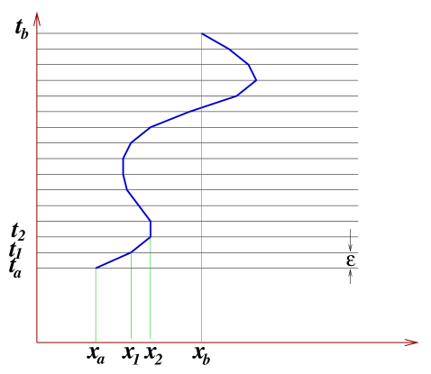
Figure 1: A typical path in the path integral for a nonrelativistic particle moving in one dimension.

2.3 Relationship to the Schrödinger equation

It is interesting to show how the above expression is equivalent to the familiar Schrödinger equation. The probability amplitude $\psi(x_{b},t_{b})$ at time $t_{b}$, assuming an amplitude $\psi(x_{a},t_{a})$ at an earlier time $t_{a}$, is given by

$$\psi(x_{b},t_{b})=\int Z(b,a)\ \psi(x_{a},t_{a})\ dx_{a}.$$

Take $t_{a}=t$ and $t_{b}=t+\varepsilon$ one time slice away, then

$$\psi(x_{b},t+\varepsilon)=\frac{1}{A}\int_{-\infty}^{\infty}\exp\left[\frac{i\varepsilon}{\hbar}L\left(\frac{x_{b}+x_{a}}{2},\frac{x_{b}-x_{a}}{\varepsilon}\right)\right]\psi(x_{a},t)\ dx_{a},$$

where in $L(x,\dot{x})$, the speed is $\dot{x}=(x_{b}-x_{a})/\varepsilon$ and the mid-point prescription $x\rightarrow(x_{b}+x_{a})/2$ is used. If the particle is subject to a potential energy, then $L=\frac{1}{2}m\dot{x}^{2}\!-\!V(x,t)$, and it is convenient to write $x_{b}=x,\ x_{a}=x+\eta$ so that

$$\psi(x,t+{\color[rgb]{1,0,0}\varepsilon})=\frac{1}{A}\int_{-\infty}^{\infty}e^{im{\color[rgb]{0,0.6,0}\eta}^{2}/(2\hbar{\color[rgb]{1,0,0}\varepsilon})}e^{-i{\color[rgb]{1,0,0}\varepsilon}V(x+{\color[rgb]{0,0.6,0}\eta}/2,t)/\hbar}\psi(x+{\color[rgb]{0,0.6,0}\eta},t)\ d{\color[rgb]{0,0.6,0}\eta}.$$

The rapid oscillation of $e^{im\eta^{2}/(2\hbar\varepsilon)}$ except when $\eta\sim O(\sqrt{\varepsilon})$ leads to the fact that the integral is dominated by contributions from $\eta$ having values of this order. Given this, we can expand all expressions to $O({\color[rgb]{1,0,0}\varepsilon})$ and $O({\color[rgb]{0,0.6,0}\eta}^{2})$, except $e^{im\eta^{2}/(2\hbar{\color[rgb]{1,0,0}\varepsilon})}$ ($\psi$ refers to $\psi(x,t)$), yielding

$$\psi+{\color[rgb]{1,0,0}\varepsilon}\frac{\partial\psi}{\partial t} = \frac{1}{A}\int_{-\infty}^{\infty}\!\!e^{im{\color[rgb]{0,0.6,0}\eta}^{2}/(2\hbar{\color[rgb]{1,0,0}\varepsilon})}\Bigl{[}1\!-\!\frac{i{\color[rgb]{1,0,0}\varepsilon}}{\hbar}V(x,t)\Bigr{]}\Bigl{[}\psi\!+\!{\color[rgb]{0,0.6,0}\eta}\frac{\partial\psi}{\partial x}+\frac{{\color[rgb]{0,0.6,0}\eta}^{2}}{2}\frac{\partial^{2}\psi}{\partial x^{2}}\Bigl{]}d{\color[rgb]{0,0.6,0}\eta},$$

$$= \frac{1}{A}\int_{-\infty}^{\infty}\!\!e^{im{\color[rgb]{0,0.6,0}\eta}^{2}/(2\hbar{\color[rgb]{1,0,0}\varepsilon})}\Bigl{[}\psi-\frac{i{\color[rgb]{1,0,0}\varepsilon}}{\hbar}V(x,t)\psi+{\color[rgb]{0,0.6,0}\eta}\frac{\partial\psi}{\partial x}+\frac{{\color[rgb]{0,0.6,0}\eta}^{2}}{2}\frac{\partial^{2}\psi}{\partial x^{2}}\Bigl{]}d{\color[rgb]{0,0.6,0}\eta}.$$

Matching the leading terms on both sides determines $A$ (using analytic continuation to evaluate the integral):

$$1=\frac{1}{A}\int_{-\infty}^{\infty}e^{im\eta^{2}/(2\hbar\varepsilon)}d\eta=\frac{1}{A}\left(\frac{2\pi i\hbar\varepsilon}{m}\right)^{1/2}\quad\Rightarrow\quad A=\left(\frac{2\pi i\hbar\varepsilon}{m}\right)^{1/2}.$$

Given the following integrals,

$$\frac{1}{A}\int_{-\infty}^{\infty}\!\!e^{im\eta^{2}/(2\hbar\varepsilon)}\,\eta\ d\eta=0,\qquad\frac{1}{A}\int_{-\infty}^{\infty}\!\!e^{im\eta^{2}/(2\hbar\varepsilon)}\,\eta^{2}d\eta=\frac{i\hbar\varepsilon}{m},$$

then the $O(\varepsilon)$ part of the equation yields

$$-\frac{\hbar}{i}\frac{\partial\psi}{\partial t}=-\frac{\hbar^{2}}{2m}\frac{\partial^{2}\psi}{\partial x^{2}}+V(x,t)\psi.$$

This is the Schrödinger equation!

2.4 Example: free particle in one dimension

Now let us explicitly evaluate the path integrals for several simple examples. First, consider a free particle of mass $m$ in one dimension. The Lagrangian of a free particle in one dimension is

$$L=\frac{1}{2}m\dot{x}^{2},$$

so the amplitude for the particle to travel from $x_{a}$ at time $t_{a}$ to location $x_{b}$ at later time $t_{b}$ is

$$\langle x_{b}(t_{b})|x_{a}(t_{a})\rangle=\int_{a}^{b}{\cal D}x(t)\exp(iS[b,a]/\hbar),$$

summing over all allowed paths with $x(t_{a})=x_{a}$ and $x(t_{b})=x_{b}$. The classical path $x_{\rm cl}(t)$ is obtained from $\delta S=0$ and boundary conditions:

$$\ddot{x}_{\rm cl}(t)=0,\qquad x_{\rm cl}(t)=x_{a}+(x_{b}-x_{a})\frac{(t-t_{a})}{(t_{b}-t_{a})},$$

and the classical action is

$$S_{\rm cl}[b,a]=\int_{t_{a}}^{t_{b}}\!\!dt\ \textstyle\frac{1}{2}m\dot{x}_{\rm cl}^{2}=\displaystyle\frac{m(x_{b}-x_{a})^{2}}{2(t_{b}-t_{a})}.$$

Write $x(t)=x_{\rm cl}(t)+\chi(t)$ with $\chi(t_{a})=\chi(t_{b})=0$, then

$$S[b,a]=S_{\rm cl}[b,a]+\int_{t_{a}}^{t_{b}}\!\!dt\ \textstyle\frac{1}{2}m\dot{\chi}^{2},$$

where $S_{\rm cl}[b,a]$ is the classical action. Notice that there are no terms linear in $\chi(t)$ since $S_{\rm cl}$ is an extremum. The transition amplitude becomes

$$Z(b,a) = F(T)\exp(iS_{\rm cl}/\hbar),$$

$$F(T) = \int_{0}^{0}\!\!{\cal D}\chi\ \exp\left\{\frac{im}{2\hbar}\int_{0}^{T}\!dt\ \dot{\chi}^{2}\right\},$$

where $T=t_{b}-t_{a}$. Partition time into discrete steps of length $\varepsilon$, use the midpoint prescription, and note that $\chi_{0}=\chi_{N}=0$:

$$\int_{0}^{0}{\cal D}\chi = \frac{1}{A}\int_{-\infty}^{\infty}\!\!\left(\prod_{l=1}^{N-1}\frac{d\chi_{l}}{A}\right),\qquad A=\left(\frac{2\pi i\hbar\varepsilon}{m}\right)^{1/2},$$

$$\int_{0}^{T}\!\!\!\!dt\ \dot{\chi}^{2} = \frac{1}{\varepsilon}\!\sum_{j=0}^{N-1}(\chi_{j+1}\!-\!\chi_{j})^{2},$$

$$F(T) = \left(\frac{m}{2\pi i\hbar\varepsilon}\right)^{N/2}\!\!\int_{-\infty}^{\infty}\!\!\left(\prod_{l=1}^{N-1}d\chi_{l}\right)\exp\left\{\frac{im}{2\hbar\varepsilon}\chi_{j}M_{jk}\chi_{k}\right\}.$$

A multivariate Gaussian integral remains:

$$F(T)=\left(\frac{m}{2\pi i\hbar\varepsilon}\right)^{N/2}\int_{-\infty}^{\infty}\!\!\left(\prod_{l=1}^{N-1}d\chi_{l}\right)\exp\left\{\frac{im}{2\hbar\varepsilon}\chi_{j}M_{jk}\chi_{k}\right\},$$

where $M$ is a symmetric $(N-1)\times(N-1)$ matrix

$$M=\left[\begin{array}[]{rrrrr}2&-1&0&0&\cdots\\ -1&2&-1&0&\cdots\\ 0&-1&2&-1&\cdots\\ \vdots&\vdots&\vdots&\vdots&\ddots\end{array}\right].$$

Gaussian integrals of a symmetric matrix $A$ are easily evaluated,

$$\int_{-\infty}^{\infty}\!\!\left(\prod_{i=1}^{n}d\chi_{i}\right)\exp\Bigl{(}-\chi_{j}A_{jk}\chi_{k}\Bigr{)}=\left(\frac{\pi^{n}}{\det A}\right)^{1/2},$$

so the result for $F(T)$ is

$$F(T)=\left(\frac{m}{2\pi i\hbar\varepsilon\det M}\right)^{1/2}.$$

We now need to compute $\det(M)$. Consider an $n\times n$ matrix $B_{n}$ of form

$$B_{n}=\left(\begin{array}[]{rrrrr}2b&-b&0&0&\cdots\\ -b&2b&-b&0&\cdots\\ 0&-b&2b&-b&\cdots\\ \vdots&\vdots&\vdots&\vdots&\ddots\end{array}\right)_{n,n}.$$

Notice that

$$\det B_{n} = 2b\det B_{n-1}+b\det\left(\begin{array}[]{c|ccc}-b&-b&0&\cdots\\ \hline\cr\begin{array}[]{c}0\\ \vdots\end{array}&\lx@intercol\hfil B_{n-2}\hfil\lx@intercol\end{array}\right),$$

$$= 2b\det B_{n-1}-b^{2}\det B_{n-2}.$$

Define $I_{n}=\det B_{n}$, then we have the recursion relation

$$I_{n+1}=2bI_{n}-b^{2}I_{n-1},\qquad I_{-1}=0,\quad I_{0}=1,\qquad n=0,1,2,\dots.$$

Rewrite $I_{n+1}=2bI_{n}-b^{2}I_{n-1},\ I_{-1}=0,\ I_{0}=1$ as

$$\left(\begin{array}[]{c}I_{n+1}\\ I_{n}\end{array}\right)=\left(\begin{array}[]{cc}2b&-b^{2}\\ 1&0\end{array}\right)\left(\begin{array}[]{c}I_{n}\\ I_{n-1}\end{array}\right)=\left(\begin{array}[]{cc}2b&-b^{2}\\ 1&0\end{array}\right)^{n}\left(\begin{array}[]{c}I_{1}\\ I_{0}\end{array}\right).$$

It is then straightforward to show that

$$\left(\begin{array}[]{cc}2b&-b^{2}\\ 1&0\end{array}\right)^{n}=\left(\begin{array}[]{cc}(n+1)b^{n}&-nb^{n+1}\\ nb^{n-1}&-(n-1)b^{n}\end{array}\right),$$

so that

$$\left(\begin{array}[]{c}I_{n+1}\\ I_{n}\end{array}\right)=\left(\begin{array}[]{cc}(n+1)b^{n}&-nb^{n+1}\\ nb^{n-1}&-(n-1)b^{n}\end{array}\right)\left(\begin{array}[]{c}2b\\ 1\end{array}\right),$$

and thus, $I_{n}=\det B_{n}=(n+1)b^{n}$. Here, $b=1$ and $n=N-1$ so $\det M=N$, and using $N\varepsilon=t_{b}-t_{a}$, we obtain

$$F(t_{b},t_{a})=\left(\frac{m}{2\pi i\hbar(t_{b}\!-\!t_{a})}\right)^{1/2}.$$

The final result for the transition amplitude for a free particle in one dimension is

$$\langle x_{b}(t_{b})|x_{a}(t_{a})\rangle=\left(\frac{m}{2\pi i\hbar(t_{b}\!-\!t_{a})}\right)^{1/2}\ \exp\left\{\frac{im(x_{b}-x_{a})^{2}}{2\hbar(t_{b}-t_{a})}\right\}.$$

2.5 Infinite square well

As a second example, consider one of the first systems usually studied when learning quantum mechanics: the infinite square well. This is a particle moving in one dimension under the influence of a potential given by

$$V(x)=\left\{\begin{array}[]{ll}0&\mbox{for $0<x<L$},\\ \infty&\mbox{for $x\leq 0$ and $x\geq L$}.\end{array}\right.$$

The path integral for the transition amplitude in this case is given by

$$Z(b,a)=\lim_{N\rightarrow\infty}\frac{1}{A}\int_{0}^{L}\!\!\!\frac{dx_{1}}{A}\cdots\int_{0}^{L}\!\!\!\frac{dx_{N-1}}{A}\ \exp\left\{\frac{im}{2\varepsilon\hbar}\sum_{j=0}^{N-1}(x_{j+1}\!-\!x_{j})^{2}\right\},$$

where the paths are limited to $0<x<L$. Gaussian integrals over bounded domains produce error functions ($\mathrm{erf}$), making direct evaluation in closed form difficult. A simple trick[2] to evaluate the path integral in this case is to extend the regions of integration to $-\infty<x<\infty$, but subtract off all forbidden paths. In so doing, we express the square well amplitude as an infinite sum of free particle amplitudes.

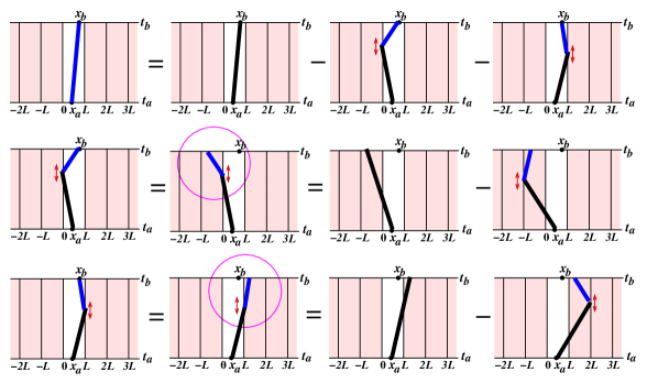
Figure 2: Expressing the set of confined paths (solid lines) of the infinite square well in terms of sets of free paths (dashed lines). The minus signs are set difference operators. Details are described in the text. The circles indicate the applications of reflections which preserve the free-particle action.

To help describe these path cancellations, let us refer to unbounded paths which can visit any value of $x$ as free paths, and we shall refer to paths which never cross an $x=nL$ boundary, for integer $n$, as confined paths. The set $S_{C}$ of all confined paths from $x_{a}$ at time $t_{a}$ to $x_{b}$ at later time $t_{b}$ is given by the set $S_{F}$ of all free paths from $x_{a}$ to $x_{b}$, excluding all free paths which cross the $x=0$ or $x=L$ boundary at least once. The set of free paths which cross the $x=0$ or $x=L$ boundary at least once can be partitioned into two non-intersecting subsets: the set $S_{1L}$ of paths whose last boundary crossing occurs at the $x=0$ boundary at time $t_{1}$, and the set $S_{1R}$ of paths whose last boundary crossing occurs at the $x=L$ boundary at time $t_{1}$, for all possible values of $t_{1}$. For a particular $t_{1}$, each subset is the set of all free paths from $x_{a}$ at $t_{a}$ to $x=0$ (or $x=L$) at time $t_{1}$ with all confined paths from $x=0$ (or $x=L)$ at $t_{1}$ to $x_{b}$ at $t_{b}$. The set expression $S_{C}=S_{F}-S_{1R}-S_{1L}$ is illustrated graphically in the top row of Fig. 2. In this figure, the solid lines represent all confined paths between the end points of the line (those that do not cross an $nL$ boundary, for integer $n$), and the dashed lines represent all free paths between the end points of the line. Remember that there is no doubling back in time. The minus signs are set difference operators.

Next, consider a particular path in set $S_{1L}$. The section of the path from $x=0$ at $t_{1}$ to $x_{b}$ at $t_{b}$ can be reflected $x\rightarrow-x$ without changing the free-particle action. This is because the free-particle Lagrangian depends only on the square of the speed which is left unchanged except at a finite number of points, a set of measure zero. Hence, as far as the path integral is concerned, the set $S_{1L}$ can be replaced by the set $S_{1L}^{\prime}$ of all free paths from $x_{a}$ at $t_{a}$ to $x=0$ at $t_{1}$ with all confined paths from $x=0$ at $t_{1}$ to $-x_{b}$ at $t_{b}$, for all possible $t_{1}$. With a little thought, one can see that $S_{1L}^{\prime}$ is the set $S_{F1L}$ of all free paths from $x_{a}$ at $t_{a}$ to $-x_{b}$ at $t_{b}$, excluding the set $S_{2L}$ of all free paths from $x_{a}$ at $t_{a}$ to $x=-L$ at $t_{1}$ with all confined paths from $x=-L$ at $t_{1}$ to $-x_{b}$ at $t_{b}$. The set expression $S_{1L}^{\prime}=S_{F1L}-S_{2L}$ is illustrated in the second row of Fig. 2.

Consider a particular path in the set $S_{1R}$. The section of the path from $x=L$ at $t_{1}$ to $x_{b}$ at $t_{b}$ can be reflected $x\rightarrow 2L-x$ without changing the free-particle action, so $S_{1R}$ can be replaced by the set $S_{1R}^{\prime}$ of all free paths from $x_{a}$ at $t_{a}$ to $x=L$ at $t_{1}$ with all confined paths from $x=L$ at $t_{1}$ to $2L-x_{b}$ at $t_{b}$, for all possible $t_{1}$. Again, it is not difficult to see that $S_{1R}^{\prime}$ is the set $S_{F1R}$ of all free paths from $x_{a}$ at $t_{a}$ to $2L-x_{b}$ at $t_{b}$, excluding the set $S_{2R}$ of all free paths from $x_{a}$ at $t_{a}$ to $x=2L$ at $t_{1}$ with all confined paths from $x=2L$ at $t_{1}$ to $2L-x_{b}$ at $t_{b}$, as illustrated in the third row of Fig. 2.

This procedure can be iterated again and again until one obtains the final result as a sum of free propagators to an infinite number of mirror points:

$$\langle x_{b},t_{b}|x_{a},t_{a}\rangle_{\rm conf}=\langle x_{b},t_{b}|x_{a},t_{a}\rangle_{\rm free}$$

$$\qquad-\langle-x_{b},t_{b}|x_{a},t_{a}\rangle_{\rm free}-\langle 2L-x_{b},t_{b}|x_{a},t_{a}\rangle_{\rm free}$$

$$\qquad+\langle-2L+x_{b},t_{b}|x_{a},t_{a}\rangle_{\rm free}+\langle 2L+x_{b},t_{b}|x_{a},t_{a}\rangle_{\rm free}+\cdots,$$

$$= \sum_{n=-\infty}^{\infty}\Bigl{\{}\langle 2nL+x_{b},t_{b}|x_{a},t_{a}\rangle_{\rm free}-\langle 2nL-x_{b},t_{b}|x_{a},t_{a}\rangle_{\rm free}\Bigr{\}}.$$

Substituting the amplitude for a free particle into this expression yields

$$\langle x_{b}(t_{b})|x_{a}(t_{a})\rangle_{\rm conf}=\left(\frac{m}{2\pi i\hbar(t_{b}-t_{a})}\right)^{1/2}$$

$$\times\sum_{n=-\infty}^{\infty}\!\!\left(\!\exp\left\{\frac{im(2nL\!+\!x_{b}\!-\!x_{a})^{2}}{2\hbar(t_{b}-t_{a})}\right\}\!-\!\ \exp\left\{\frac{im(2nL\!-\!x_{b}\!-\!x_{a})^{2}}{2\hbar(t_{b}-t_{a})}\right\}\right).$$

Apply Poisson summation and integrate the Gaussian

$$\sum_{n=-\infty}^{\infty}f(n)=\sum_{j=-\infty}^{\infty}\int_{-\infty}^{\infty}\!ds\ f(s)e^{2\pi ijs},$$

$$\int_{-\infty}^{\infty}\!\!ds\exp\Bigl{(}-i\alpha s^{2}\pm i\beta s\Bigr{)}=\sqrt{\frac{\pi}{i\alpha}}\exp\left(\frac{i\beta^{2}}{4\alpha}\right),$$

to finally obtain the spectral representation of the transition amplitude for an infinite square well:

$$\langle x_{b}(t_{b})|x_{a}(t_{a})\rangle_{\rm well}=\sum_{n=1}^{\infty}\varphi_{n}(x_{b})\varphi^{\ast}_{n}(x_{a})e^{-iE_{n}(t_{b}-t_{a})/\hbar},$$

$$E_{n}=\frac{n^{2}\pi^{2}\hbar^{2}}{2mL^{2}},\qquad\varphi_{n}(x)=\sqrt{\frac{2}{L}}\sin\left(\frac{n\pi x}{L}\right).$$

The familiar energy levels and wavefunctions have been obtained using only path integrals.

2.6 Free particle in 1D periodic box

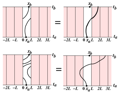
Figure 3: Each path in the periodic box is equivalent to a free path leading to an appropriate mirror point. The equivalent free path is found by horizontally translating sections of the periodic path to form a continuous free path.

For our third example, consider a particle moving in one dimension with periodic boundary conditions at $x=0$ and $x=L$. Once again, directly enforcing boundary conditions on the path integrals is difficult, so it is best to proceed by using a trick similar to that used for the infinite square well, that is, to express the set of allowed paths in terms of an equivalent set of unrestricted paths. Each path in the periodic box is equivalent to a free path leading to an appropriate mirror point. The equivalent free path is found by horizontally translating sections of the periodic path to form a continuous free path, as shown in Fig. 3. The resulting amplitude is a sum of free amplitudes to an infinite number of mirror points:

$$\langle x_{b},t_{b}|x_{a},t_{a}\rangle_{\rm periodic}=\sum_{n=-\infty}^{\infty}\langle x_{b}+nL,t_{b}|x_{a},t_{a}\rangle_{\rm free}.$$

Substitute the amplitude for a free particle,

$$\langle x_{b}(t_{b})|x_{a}(t_{a})\rangle=\left(\frac{m}{2\pi i\hbar(t_{b}-t_{a})}\right)^{1/2}\sum_{n=-\infty}^{\infty}\!\!\exp\left\{\frac{im(nL\!+\!x_{b}\!-\!x_{a})^{2}}{2\hbar(t_{b}-t_{a})}\right\},$$

apply Poisson summation, and integrate the Gaussian,

$$\sum_{n=-\infty}^{\infty}f(n)=\sum_{j=-\infty}^{\infty}\int_{-\infty}^{\infty}\!ds\ f(s)e^{2\pi ijs},$$

$$\int_{-\infty}^{\infty}\!\!ds\exp\Bigl{(}-i\alpha s^{2}\pm i\beta s\Bigr{)}=\sqrt{\frac{\pi}{i\alpha}}\exp\left(\frac{i\beta^{2}}{4\alpha}\right),$$

to obtain the spectral representation of the transition amplitude:

$$\langle x_{b}(t_{b})|x_{a}(t_{a})\rangle=\sum_{n=-\infty}^{\infty}\varphi_{n}(x_{b})\varphi^{\ast}_{n}(x_{a})e^{-iE_{n}(t_{b}-t_{a})/\hbar},$$

$$E_{n}=\frac{p_{n}^{2}}{2m},\qquad p_{n}=\frac{2\pi n\hbar}{L},\qquad\varphi_{n}(x)=\frac{1}{\sqrt{L}}e^{ip_{n}x/\hbar}.$$

The quantization of the momentum, and the familiar energy levels and wavefunctions have once again emerged using only path integrals.

2.7 Simple harmonic oscillator in 1D

The one-dimensional simple harmonic oscillator is our last example. The kinetic and potential energies of a simple harmonic oscillator of mass $m$ and frequency $\omega$ are given by

$$K=\textstyle\frac{1}{2}m\dot{x}^{2},\qquad U=\frac{1}{2}m\omega^{2}x^{2},$$

so the action is

$$S[x(t)]=\int_{t_{a}}^{t_{b}}\!dt\ \left(\textstyle\frac{1}{2}m\dot{x}^{2}-\frac{1}{2}m\omega^{2}x^{2}\right).$$

The classical equations of motion are

$$\delta S=0\quad\Rightarrow\quad\ddot{x}_{\rm cl}+\omega^{2}x_{\rm cl}=0,$$

and the value of action for the classical path is

$$S_{\rm cl}=\frac{m\omega}{2\sin(\omega T)}\Biggl{[}(x_{a}^{2}+x_{b}^{2})\cos(\omega T)-2x_{a}x_{b}\Biggr{]},$$

where $T=t_{b}-t_{a}$. To calculate the amplitude $Z(b,a)=\langle x_{b}(t_{b})|x_{a}(t_{a})\rangle_{\rm sho}$, write the path as a deviation from the classical path:

$$x(t)=x_{\rm cl}(t)+\chi(t),\qquad\chi(t_{a})=\chi(t_{b})=0.$$

The amplitude can then be written as

$$Z(b,a) = F(T)\exp(iS_{\rm cl}/\hbar),$$

$$F(T) = \int_{0}^{0}\!\!{\cal D}\chi\ \exp\left\{\frac{im}{2\hbar}\int_{0}^{T}\!dt\ (\dot{\chi}^{2}-\omega^{2}\chi^{2})\right\}.$$

Partition time into discrete steps of length $\varepsilon$ and use a midpoint prescription:

$$\int_{0}^{0}{\cal D}\chi\!\! = \frac{1}{A}\int_{-\infty}^{\infty}\!\!\left(\prod_{l=1}^{N-1}\frac{d\chi_{l}}{A}\right),\qquad A=\left(\frac{2\pi i\hbar\varepsilon}{m}\right)^{1/2},$$

$$\int_{0}^{T}\!\!dt(\dot{\chi}^{2}\!-\!\omega^{2}\chi^{2}) = \frac{1}{\varepsilon}\!\sum_{j=0}^{N-1}\left[(\chi_{j+1}\!-\!\chi_{j})^{2}\!-\!\frac{\varepsilon^{2}\omega^{2}}{4}(\chi_{j+1}\!+\!\chi_{j})^{2}\right],$$

$$F(T) = \left(\frac{m}{2\pi i\hbar\varepsilon}\right)^{N/2}\!\!\!\int_{-\infty}^{\infty}\!\!\left(\prod_{l=1}^{N-1}d\chi_{l}\right)\exp\left\{\frac{im}{2\hbar\varepsilon}\chi_{j}M_{jk}\chi_{k}\right\}.$$

A multivariate Gaussian integral remains:

$$F(T)=\left(\frac{m}{2\pi i\hbar\varepsilon}\right)^{N/2}\int_{-\infty}^{\infty}\!\!\left(\prod_{l=1}^{N-1}d\chi_{l}\right)\exp\left\{\frac{im}{2\hbar\varepsilon}\chi_{j}M_{jk}\chi_{k}\right\},$$

where $M$ is a symmetric $(N-1)\times(N-1)$ matrix

$$M=\left[\begin{array}[]{rrrrr}2&-1&0&0&\cdots\\ -1&2&-1&0&\cdots\\ 0&-1&2&-1&\cdots\\ \vdots&\vdots&\vdots&\vdots&\ddots\end{array}\right]-\frac{\varepsilon^{2}\omega^{2}}{4}\left[\begin{array}[]{rrrrr}2&1&0&0&\cdots\\ 1&2&1&0&\cdots\\ 0&1&2&1&\cdots\\ \vdots&\vdots&\vdots&\vdots&\ddots\end{array}\right].$$

Such Gaussian integrals are easily evaluated:

$$F(T)=\left(\frac{m}{2\pi i\hbar\varepsilon\det M}\right)^{1/2}.$$

Now we must compute $\det M$. Consider $\det(B_{n})$, where the $n\times n$ matrix $B_{n}$ has the form

$$B_{n}=\left(\begin{array}[]{ccccc}a&b&0&0&\cdots\\ b&a&b&0&\cdots\\ 0&b&a&b&\cdots\\ \vdots&\vdots&\vdots&\vdots&\ddots\end{array}\right)_{n,n}.$$

$B_{n}$ matches $M$ for $n=N-1$, $a=2(1-\epsilon^{2}\omega^{2}/4)$, and $b=-(1+\epsilon^{2}\omega^{2}/4)$. Notice that

$$\det B_{n} = a\det B_{n-1}-b\det\left(\begin{array}[]{c|ccc}b&b&0&\cdots\\ \hline\cr\begin{array}[]{c}0\\ \vdots\end{array}&\lx@intercol\hfil B_{n-2}\hfil\lx@intercol\end{array}\right),$$

$$= a\det B_{n-1}-b^{2}\det B_{n-2}.$$

Define $I_{n}=\det B_{n}$ to obtain the recursion relation

$$I_{n+1}=aI_{n}-b^{2}I_{n-1},\qquad I_{-1}=0,\quad I_{0}=1,\qquad n=0,1,2,\dots.$$

Rewrite this recursion relation as

$$\left(\begin{array}[]{c}I_{n+1}\\ I_{n}\end{array}\right)=\left(\begin{array}[]{cc}a&-b^{2}\\ 1&0\end{array}\right)\left(\begin{array}[]{c}I_{n}\\ I_{n-1}\end{array}\right)=\left(\begin{array}[]{cc}a&-b^{2}\\ 1&0\end{array}\right)^{n}\left(\begin{array}[]{c}I_{1}\\ I_{0}\end{array}\right),$$

diagonalize as follows,

$$\left(\begin{array}[]{cc}a&-b^{2}\\ 1&0\end{array}\right)={\cal S}\ \left(\begin{array}[]{cc}\lambda_{+}&0\\ 0&\lambda_{-}\end{array}\right)\ {\cal S}^{-1},$$

$$\lambda_{\pm}=\frac{1}{2}\Bigl{(}a\pm\sqrt{a^{2}-4b^{2}}\Bigr{)},$$

$${\cal S}=\left(\begin{array}[]{cc}\lambda_{+}&\lambda_{-}\\ 1&1\end{array}\right),\quad{\cal S}^{-1}=\frac{1}{\lambda_{+}-\lambda_{-}}\left(\begin{array}[]{cc}1&-\lambda_{-}\\ -1&\lambda_{+}\end{array}\right),$$

then we have

$$\left(\begin{array}[]{c}I_{n+1}\\ I_{n}\end{array}\right)={\cal S}\left(\begin{array}[]{cc}\lambda_{+}^{n}&0\\ 0&\lambda_{-}^{n}\end{array}\right){\cal S}^{-1}\left(\begin{array}[]{c}a\\ 1\end{array}\right).$$

Thus,

$$I_{n}=\det B_{n}=\frac{\lambda_{+}^{n+1}-\lambda_{-}^{n+1}}{\lambda_{+}-\lambda_{-}},\qquad(\lambda_{+}\neq\lambda_{-}).$$

Using $\lambda_{\pm}=1\pm i\omega\epsilon+O(\varepsilon^{2})$ yields

$$\lim_{\genfrac{}{}{0.0pt}{}{\varepsilon\rightarrow 0}{N\rightarrow\infty}}\varepsilon\det M = \lim_{\genfrac{}{}{0.0pt}{}{\varepsilon\rightarrow 0}{N\rightarrow\infty}}\varepsilon\frac{1}{2i\omega\varepsilon}\Bigl{(}(1+i\omega\varepsilon)^{N}-(1-i\omega\varepsilon)^{N}\Bigr{)},$$

$$= \lim_{\genfrac{}{}{0.0pt}{}{\varepsilon\rightarrow 0}{N\rightarrow\infty}}\frac{1}{2i\omega}\left(\left(1+\frac{i\omega T}{N}\right)^{N}-\left(1-\frac{i\omega T}{N}\right)^{N}\right),$$

$$= \frac{1}{2i\omega}\left(e^{i\omega T}-e^{-i\omega T}\right)=\frac{\sin\omega T}{\omega}.$$

The final result for the path integral is

$$\langle x_{b}(t_{b})|x_{a}(t_{a})\rangle_{\rm sho}=\left(\frac{m\omega}{2\pi i\hbar\sin\bigl{(}\omega(t_{b}\!-\!t_{a})\bigr{)}}\right)^{1/2}\ \exp\Bigl{\{}iS_{\rm cl}/\hbar\Bigr{\}}.$$

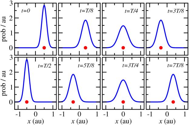
Figure 4: Time evolution of a Gaussian wave packet for a simple harmonic oscillator of mass $m=1\mathrm{g/mol}=1.66\times 10^{-27}\mathrm{kg}$ and frequency $\omega=3\times 10^{14}\mathrm{radians/sec}$. The initial wave packet at $t=0$ is centered at 0.5 au and has initial width $\sigma=$0.14 au. Note that 1 au (atomic unit) = 0.529 angstrom. The dot indicates the location of a classical oscillator of the same mass and frequency. The probabilities are shown for times $t=nT/8$ for $n=0,1,2,\dots,7$, where $T$ is the period.

Consider the temporal evolution of a Gaussian wave packet for this system. If the probability distribution corresponding to the initial wave packet at time $t_{a}=0$ is a Gaussian:

$$|\phi(x_{a},t_{a})|^{2}=\frac{1}{\sigma\sqrt{2\pi}}\exp\left(-\frac{(x_{a}-\bar{x})^{2}}{2\sigma^{2}}\right),$$

then the probability amplitude at a later time $t_{b}$ is

$$\phi(x_{b},t_{b}) = \int_{-\infty}^{\infty}\!\!\!\!\!dx_{a}\ Z(b,a)\ \phi(x_{a},0),$$

$$= \left(\frac{-im\omega(2\pi)^{-3/2}}{\hbar\sigma\sin(\omega t_{b})}\right)^{1/2}\!\!\!\!\int_{-\infty}^{\infty}\!\!\!\!\!dx_{a}\ e^{iS_{\rm cl}/\hbar}\ e^{-(x_{a}-\bar{x})^{2}/(4\sigma^{2})},$$

so the probability distribution remains a Gaussian but with a varying width $s(t)$:

$$|\phi(x_{b},t_{b})|^{2}=\frac{1}{s(t_{b})\sqrt{2\pi}}\exp\left(-\frac{(x_{b}-\bar{x}\cos(\omega t_{b}))^{2}}{2s^{2}(t_{b})}\right),$$

where the width is given by

$$s(t_{b})=\sigma\left\{\cos^{2}(\omega t_{b})+\frac{\hbar^{2}}{4m^{2}\omega^{2}\sigma^{4}}\sin^{2}(\omega t_{b})\right\}^{1/2}.$$

The time evolution of such a Gaussian wave packet for a simple harmonic oscillator is shown in Fig. 4. Note that this evolution was completely calculated above using path integrals; the Schrödinger equation was not used.

2.8 Correlation functions and observables

We have so far seen that path integrals give us simple transition amplitudes, such as

$$\langle x_{b}(t_{b})|x_{a}(t_{a})\rangle=\int_{a}^{b}\!\!{\cal D}x\ \exp\left\{\frac{i}{\hbar}\int_{t_{a}}^{t_{b}}\!\!dt\ L(x,\dot{x})\right\},$$

but this important result generalizes to more complicated amplitudes:

$$\langle x_{b}(t_{b})|\ x(t_{2})\ x(t_{1})\ |x_{a}(t_{a})\rangle,$$

$$= \int_{a}^{b}\!\!{\cal D}x\ x(t_{2})x(t_{1})\ \exp\left\{\frac{i}{\hbar}\int_{t_{a}}^{t_{b}}\!\!dt\ L(x,\dot{x})\right\},$$

for $t_{a}<t_{1}<t_{2}<t_{b}$. In the imaginary time formalism, paths contribute to the sum over histories with real exponential weights (not phases):

$$\langle x_{b}(\tau_{b})|\ x(\tau_{2})\ x(\tau_{1})\ |x_{a}(\tau_{a})\rangle$$

$$= \int_{a}^{b}\!\!{\cal D}x\ x(\tau_{2})x(\tau_{1})\ \exp\left\{-\frac{1}{\hbar}\int_{\tau_{a}}^{\tau_{b}}\!\!d\tau\ L(x,\dot{x})\right\}.$$

Now the classical path gets the highest weighting. Note that weights are all real and positive since the action is real. This fact will be crucial for the Monte Carlo method.

Another important fact is that correlation functions (vacuum expectation values) can be obtained from ratios of path integrals. For example, a two-point function can be obtained from

$$\langle 0|{\color[rgb]{1,0,1}x(t_{2})x(t_{1})}|0\rangle=\lim_{T\rightarrow\infty}\frac{\langle{\color[rgb]{0,0.6,0}x_{b}(T)}|{\color[rgb]{1,0,1}x(t_{2})x(t_{1})}|{\color[rgb]{1,0,0}x_{a}(-T)}\rangle}{\langle{\color[rgb]{0,0.6,0}x_{b}(T)}|{\color[rgb]{1,0,0}x_{a}(-T)}\rangle},$$

$$= \frac{\displaystyle\int_{a}^{b}{\cal D}x\ {\color[rgb]{1,0,1}x(t_{2})x(t_{1})}\exp\left\{-\frac{1}{\hbar}\int_{-\infty}^{\infty}\!d\tau L(x,\dot{x})\right\}}{\displaystyle\int_{a}^{b}{\cal D}x\ \exp\left\{-\frac{1}{\hbar}\int_{-\infty}^{\infty}\!d\tau L(x,\dot{x})\right\}},$$

and more complicated correlation functions can similarly be obtained. In fact, any correlation function can be computed using path integrals.

For example, consider the simple harmonic oscillator. Evaluating path integrals as before, the following correlation functions can be obtained:

$$\langle 0|x(\tau_{1})|0\rangle = 0,$$

$$\langle 0|x(\tau_{2})x(\tau_{1})|0\rangle = \frac{\hbar}{2m\omega}e^{-\omega(\tau_{2}\!-\!\tau_{1})},$$

$$\langle 0|x(\tau_{4})x(\tau_{3})x(\tau_{2})x(\tau_{1})|0\rangle = \left(\frac{\hbar}{2m\omega}\right)^{2}e^{-\omega(\tau_{4}\!-\!\tau_{1})}\Bigl{[}e^{-\omega(\tau_{2}\!-\!\tau_{3})}+2e^{-\omega(\tau_{3}\!-\!\tau_{2})}\Bigr{]},$$

where $\tau_{1}\leq\tau_{2}\leq\tau_{3}\leq\tau_{4}$. Comparison with the spectral representations tells us

$$\langle 0|x(\tau)x(0)|0\rangle=\frac{\hbar}{2m\omega}e^{-\omega\tau}\ \Rightarrow\ E_{1}-E_{0}=\hbar\omega,\quad|\langle 1|x(0)|0\rangle|^{2}=\frac{\hbar}{2m\omega}.$$

As another example in the SHO case, consider exciting the vacuum with the $x(\tau)^{2}$ operator:

$$\langle 0|x^{2}(\tau)x^{2}(0)|0\rangle=\left(\frac{\hbar}{2m\omega}\right)^{2}\biggl{(}1+2e^{-2\omega\tau}\biggr{)}.$$

Compare with the spectral representation at large time separations,

$$\lim_{\tau\rightarrow\infty}\langle 0|x^{2}(\tau)x^{2}(0)|0\rangle = |\langle 0|x^{2}(0)|0\rangle|^{2}+|\langle 2|x^{2}(0)|0\rangle|^{2}\ e^{-(E_{2}-E_{0})t/\hbar}+\dots,$$

$$= \left(\frac{\hbar}{2m\omega}\right)^{2}\biggl{(}1+2e^{-2\omega\tau}\biggr{)},$$

to arrive at the following interpretation:

$$E_{2}-E_{0}=2\hbar\omega,$$

$$|\langle 0|x^{2}(0)|0\rangle|^{2}=\left(\frac{\hbar}{2m\omega}\right)^{2},\qquad|\langle 2|x^{2}(0)|0\rangle|^{2}=2\left(\frac{\hbar}{2m\omega}\right)^{2}.$$

One last example in the SHO: to determine the expectation value of $x(0)^{2}$ in first-excited state, evaluate

$$\langle 0|x(\tau)\ x^{2}({\textstyle\frac{1}{2}}\tau)\ x(0)|0\rangle=3\left(\frac{\hbar}{2m\omega}\right)^{2}\ e^{-\omega\tau},$$

and compare with its spectral interpretation at large times:

$$\lim_{\tau\rightarrow\infty}\langle 0|x(\tau)x^{2}(\textstyle\frac{1}{2}\tau)x(0)|0\rangle$$

$$\qquad=|\langle 0|x(0)|1\rangle|^{2}\langle 1|x^{2}(0)|1\rangle\ e^{-(E_{1}-E_{0})\tau/\hbar}+\cdots,$$

since $\langle 0|x(0)|0\rangle=\langle 0|x(\tau)|0\rangle=0$. By inspection and using previously derived results, one concludes that

$$\langle 1|x^{2}(0)|1\rangle=\frac{3\hbar}{2m\omega}.$$

Now pause for reflection. We have seen that observables in quantum mechanics can be extracted from correlation functions (vacuum expectation values), and that the imaginary time formalism is a great trick for assisting in such extractions. Correlation functions can be computed via ratios of path integrals

$$\langle 0|{\color[rgb]{1,0,1}x(t_{2})x(t_{1})}|0\rangle$$

$$= \frac{\displaystyle\int_{a}^{b}{\cal D}x\ {\color[rgb]{1,0,1}x(t_{2})x(t_{1})}\exp\left\{-\frac{1}{\hbar}\int_{-\infty}^{\infty}\!d\tau L(x,\dot{x})\right\}}{\displaystyle\int_{a}^{b}{\cal D}x\ \exp\left\{-\frac{1}{\hbar}\int_{-\infty}^{\infty}\!d\tau L(x,\dot{x})\right\}}.$$

3 Monte Carlo integration and Markov chains

In rare situations, the path integrals in transition amplitudes can be computed exactly, such as the simple harmonic oscillator and a free particle. Sometimes the action can be written $S=S_{0}+gS_{I}$, where $S_{0}$ describes the free motion of the particles and $S_{I}$ describes the interactions of the particles, but the coupling $g$ is small. Typically, the path integrals using $S_{0}$ are Gaussian and can be exactly computed, and the interactions can be taken into account using perturbation theory as an expansion in $g$. However, if the interactions are not weak, such as in quantum chromodynamics, one must somehow numerically evaluate the needed path integrals with powerful computers.

The trapezoidal rule and Simpson’s rule are not feasible for integrals of very large dimension. These methods require far too many function evaluations. One of the most productive ways of proceeding is to start gambling! The Monte Carlo method comes to our rescue. The basic theorem of Monte Carlo integration is

$$\int_{\cal V}f(\vec{x})\ d^{D}x\approx{\cal V}\langle f\rangle\pm{\cal V}\sqrt{\frac{\langle f^{2}\rangle-\langle f\rangle^{2}}{N}},$$

$$\langle f\rangle\equiv\frac{1}{N}\sum_{i=1}^{N}f(\vec{x}_{i}),\qquad\qquad\langle f^{2}\rangle\equiv\frac{1}{N}\sum_{i=1}^{N}f(\vec{x}_{i})^{2},$$

where the $N$ points $\vec{x}_{1},\dots,\vec{x}_{N}$ are chosen independently and randomly with a uniform probability distribution throughout the $D$-dimensional volume ${\cal V}$. The method is justified by the law of large numbers and the central limit theorem. In the limit $N\rightarrow\infty$, the above Monte Carlo estimate tends to a normal distribution and the uncertainty tends to a standard deviation.

The above method sounds too good to be true. Although the above method should work in principle, it is impractical for evaluating quantum mechanical path integrals, unless suitably modified to incorporate importance sampling. Before discussing this, a closer look at the simple Monte Carlo method is warranted, and this can be facilitated with a quick review of probability theory.

3.1 Quick review of probabilities

Consider an experiment whose outcome depends on chance. Represent an outcome by $X$ called a random variable, and the sample space $\Omega$ of the experiment is the set of all possible outcomes. $X$ is called discrete if $\Omega$ is finite or countably infinite, and continuous otherwise. The probability distribution for discrete $X$ is a real-valued function $p_{X}$ on the domain $\Omega$ satisfying $p_{X}(x)\geq 0$ for all $x\in\Omega$ and $\sum_{x\in\Omega}p_{X}(x)=1$. For any subset $E$ of $\Omega$, the probability of $E$ is $P(E)=\sum_{x\in E}p_{X}(x)$. A sequence of random variables $X_{1},X_{2},\dots,X_{N}$ that are mutually independent and have the same probability distribution is called an independent trials process.

For a continuous real-valued $X$, the real-valued function $p_{X}$ is a probability density and the probability of an outcome between real values $a$ and $b$ is $P(a\leq X\leq b)=\int_{a}^{b}p_{X}(s)ds$. The cumulative distribution is $F_{X}(x)=P(X\leq x)=\int_{-\infty}^{x}p_{X}(s)ds$. A common probability density is the normal distribution $p_{X}(x)=\displaystyle\frac{1}{\sqrt{2\pi}\sigma}e^{-(x-\mu)^{2}/(2\sigma^{2})}$.

The expected value of $X$ is

$$E(X)=\sum_{x\in\Omega}x\ p_{X}(x)\qquad\left(=\int_{-\infty}^{\infty}s\ p_{X}(s)ds\right).$$

The expected value satisfies $E(X+Y)=E(X)+E(Y)$ and $E(cX)=cE(X)$, and for independent random variables $X,Y$ one has $E(XY)=E(X)E(Y)$. One can show that $E(X)$ is the average of outcomes if repeated many times. For a continuous real-valued function $f$, one can also show that

$$E(f(X))=\sum_{x\in\Omega}f(x)\ p_{X}(x)\qquad\left(=\int_{-\infty}^{\infty}f(s)\ p_{X}(s)\,ds\right).$$

To see this, group together terms in $\sum_{x}\!f(x)p_{X}(x)$ having same $f(x)$ value. Denote the set of different $f(x)$ values by ${\cal F}$, and the subset of $\Omega$ leading to same value of $f(x)$ by $\Omega_{f(x)}$, then

$$\sum_{x\in\Omega}f(x)p_{X}(x)=\sum_{y\in{\cal F}}\sum_{x\in\Omega_{f(x)}}\!\!f(x)p_{X}(x)=\sum_{y\in{\cal F}}y\,(\!\!\sum_{x\in\Omega_{f(x)}}\!\!\!p_{X}(x))$$

$$=\sum_{y\in{\cal F}}yp(y)=E(f(x)).$$

The variance of $X$ is $V(X)=E(\ (X-E(X))^{2}\ )$, and the standard deviation of $X$ is $\sigma(X)=\sqrt{V(X)}$. The variance satisfies $V(cX)=c^{2}V(X)$ and $V(X+c)=V(X)$, and for independent random variables $X,Y$, one has $V(X+Y)=V(X)+V(Y)$. Let $X_{1},\dots,X_{N}$ be an independent trials process with $E(X_{j})=\mu$ and $V(X_{j})=\sigma^{2}$, and define $A_{N}=(X_{1}+X_{2}+\dots+X_{N})/N$, then one can easily show

$$E(A_{N})=\mu,\qquad V(A_{N})=\sigma^{2}/N.$$

An important theorem in probability and statistics is known as Chebyshev’s inequality: Let $X$ be a random variable (discrete or continuous) with $E(X)=\mu$ and let $\epsilon>0$ be any positive real number, then

$$P(|X-\mu|\geq\epsilon)\leq\frac{V(X)}{\epsilon^{2}}.$$

Proof 3.1.

Let $p_{X}(x)$ denote the probability distribution of $X$, then the probability that $X$ differs from $\mu$ by at least $\epsilon$ is

$$\qquad\qquad P(|X-\mu|\geq\epsilon)=\sum_{|x-\mu|\geq\epsilon}p_{X}(x).$$

Considering the ranges of summation and that we have positive summands,

$$V(X)=\sum_{x}(x-\mu)^{2}p_{X}(x)\geq\sum_{|x-\mu|\geq\epsilon}(x-\mu)^{2}p_{X}(x)\geq\sum_{|x-\mu|\geq\epsilon}\epsilon^{2}p_{X}(x),$$

but the rightmost expression is

$$\epsilon^{2}\sum_{|x-\mu|\geq\epsilon}p_{X}(x)=\epsilon^{2}P(|X-\mu|\geq\epsilon).$$

Thus, we have shown $V(x)\geq\epsilon^{2}P(|X-\mu|\geq\epsilon)$.

An important consequence of Chebyshev’s inequality is the weak law of large numbers: Let $X_{1},X_{2},\dots,X_{N}$ be an independent trials process with $E(X_{j})=\mu$ and $V(X_{j})=\sigma^{2}$, where $\mu,\sigma$ are finite, and let $A_{N}=(X_{1}+X_{2}+\dots+X_{N})/N$. Then for any $\epsilon>0$,

$$\lim_{N\rightarrow\infty}P(|A_{N}-\mu|\geq\epsilon)=0,\qquad\lim_{N\rightarrow\infty}P(|A_{N}-\mu|<\epsilon)=1.$$

Proof 3.2.

We previously stated that $E(A_{N})=\mu$ and $V(A_{N})=\sigma^{2}/N$, and from the Chebyshev inequality,

$$P(|A_{N}-\mu|\geq\epsilon)\leq\frac{V(A_{N})}{\epsilon^{2}}=\frac{\sigma^{2}}{N\epsilon^{2}}\stackrel{{\scriptstyle N\rightarrow\infty}}{{\longrightarrow}}0.$$

This is also known as the law of averages, and applies to continuous random variables as well.

A different version of the above law is known as the strong law of large numbers: Let $X_{1},X_{2},\dots,X_{N}$ be an independent trials process with $E(X_{j})=\mu$ and $V(X_{j}^{2})=\sigma^{2}$, where $\mu,\sigma$ are finite, then

$$P\left(\lim_{N\rightarrow\infty}(X_{1}+X_{2}+\dots+X_{N})/N=\mu\right)=1.$$

Proof 3.3.

We shall assume that the random variables $X_{j}$ have a finite fourth moment $E(X_{j}^{4})=K<\infty$. The finiteness of $E(X_{j}^{4})$ is not needed, but simplifies the proof. For a proof without this assumption, see Ref. etemadi.

Define $Y_{j}=X_{j}-\mu$ so $E(Y_{j})=0$. Define $B=E(Y_{i}^{2})<\infty$ and $C=E(Y_{j}^{4})<\infty$, then define $A_{N}=(Y_{1}+Y_{2}+\dots+Y_{N})/N$. Consider

$$N^{4}E(A_{N}^{4})=E(\,(Y_{1}+Y_{2}+\cdots+Y_{N})^{4}\,).$$

Expanding $A_{N}^{4}$ yields terms of the form $Y_{i}^{4}$, $Y_{i}^{3}Y_{j}$, $Y_{i}^{2}Y_{j}^{2}$, $Y_{i}^{2}Y_{j}Y_{k}$, and $Y_{i}Y_{j}Y_{k}Y_{l}$, where $i,j,k,l$ are all different. Given that $E(Y_{j})=0$ and all $Y_{j}$ are independent, then

$$E(Y_{i}^{3}Y_{j}) = E(Y_{i}^{3})E(Y_{j})=0,\qquad\mbox{($i,j,k,l$ all different)}$$

$$E(Y_{i}^{2}Y_{j}Y_{k}) = E(Y_{i}^{2})E(Y_{j})E(Y_{k})=0,$$

$$E(Y_{i}Y_{j}Y_{k}Y_{l}) = E(Y_{i})E(Y_{j})E(Y_{k})E(Y_{l})=0,$$

$$E(Y_{i}^{2}Y_{j}^{2}) = E(Y_{i}^{2})E(Y_{j}^{2})=B^{2}.$$

Since the random variables are identically distributed, then $E(Y_{i}^{4})$ and $E(Y_{i}^{2}Y_{j}^{2})$ are independent of $i,j$, so we have

$$N^{4}E(A_{N}^{4})=NE(Y_{j}^{4})+6\textstyle\genfrac{(}{)}{0.0pt}{}{N}{2}E(Y_{i}^{2}Y_{j}^{2})=NC+3N(N-1)B^{2}.$$

Since $0\leq V(Y_{j}^{2})=E((Y_{j}^{2}-E(Y_{j}^{2})^{2})=E(Y_{j}^{4})-E(Y_{j}^{2})^{2}$ then $B^{2}=E(Y_{j}^{2})^{2}\leq E(Y_{j}^{4})=C$ so $E(A_{N}^{4})\leq C/N^{3}+3C/N^{2}$, which means

$$E\left(\sum_{N=1}^{\infty}A_{N}^{4}\right)=\sum_{N=1}^{\infty}E(A_{N}^{4})\leq\sum_{N=1}^{\infty}\left(\frac{C}{N^{3}}+\frac{3C}{N^{2}}\right)<\infty.$$

This implies $\sum_{N=1}^{\infty}A_{N}^{4}<\infty$ with unit probability, and convergence of this series implies $\lim_{N\rightarrow\infty}A_{N}^{4}=0$, which means that $\lim_{N\rightarrow\infty}A_{N}=0$.

This proves that $E(X)$ is the average of outcomes for many repetitions.

Uncertainties in Monte Carlo estimates depend upon the celebrated central limit theorem: Let $X_{1},X_{2},\dots,X_{N}$ be independent random variables with common distribution having $E(X_{j})=\mu$ and $V(X_{j})=\sigma^{2}$, where $\mu,\sigma$ are finite, and let $A_{N}=(X_{1}+X_{2}+\dots+X_{N})/N$. Then for $a<b$,

$$\lim_{N\rightarrow\infty}P\left(\frac{a\sigma}{\sqrt{N}}<(A_{N}-\mu)<\frac{b\sigma}{\sqrt{N}}\right)=\frac{1}{\sqrt{2\pi}}\int_{a}^{b}e^{-x^{2}/2}dx.$$

Alternatively, the distribution of $(X_{1}+\dots+X_{N}-N\mu)/(\sigma\sqrt{N})$ tends to the standard normal (zero mean, unit variance).

Proof 3.4.

Define $S_{N}=N(A_{N}-\mu)/(\sigma\sqrt{N})$, and if $t$ is a real-valued parameter, then

$$E\left(e^{tS_{N}}\right) = E\left(e^{t(X_{1}-\mu)/(\sigma\sqrt{N})}e^{t(X_{2}-\mu)/(\sigma\sqrt{N})}\cdots e^{t(X_{N}-\mu)/(\sigma\sqrt{N})}\right),$$

$$= E\left(\!e^{t(X_{1}-\mu)/(\sigma\sqrt{N})}\!\right)E\left(\!e^{t(X_{2}-\mu)/(\sigma\sqrt{N})}\!\right)\cdots E\left(\!e^{t(X_{N}-\mu)/(\sigma\sqrt{N})}\!\right),$$

$$= \left[E\left(e^{t(X_{1}-\mu)/(\sigma\sqrt{N})}\right)\right]^{N},$$

where, in the last two steps above, we used, respectively, the facts that the $X_{j}$ are independent and are identically distributed. Now carry out a Taylor series expansion about $t=0$:

$$E\left(\!e^{t(X_{1}\!-\!\mu)/(\sigma\sqrt{N})}\!\right) = E\left(1+\frac{t(X_{1}-\mu)}{\sigma\sqrt{N}}\ +\frac{t^{2}(X_{1}-\mu)^{2}}{2\sigma^{2}N}+\cdots\right),$$

$$= E(1)+\frac{t}{\sigma\sqrt{N}}E(X_{1}\!-\!\mu)+\frac{t^{2}}{2\sigma^{2}N}E\left((X_{1}\!-\!\mu)^{2}\right)+\cdots,$$

$$= 1+\frac{t}{\sigma\sqrt{N}}(0)+\frac{t^{2}}{2\sigma^{2}N}\sigma^{2}+\cdots=1+\frac{t^{2}}{2N}+\cdots.$$

From this, one sees that

$$\lim_{N\rightarrow\infty}E\left(\!e^{t(X_{1}\!-\!\mu)/(\sigma\sqrt{N})}\!\right)=\lim_{N\rightarrow\infty}\left(1+\frac{t^{2}}{2N}+\cdots\right)^{N}=e^{t^{2}/2}.$$

This is the moment generating function of the standardized normal distribution. The moment generating function of a random variable $X$ is defined by $M_{X}(t)=E(e^{tX})$. If $X$ and $Y$ are random variables having moment generating functions $M_{X}(t)$ and $M_{Y}(t)$, respectively, then there is a uniqueness theorem that states that $X$ and $Y$ have the same probability distribution if and only if $M_{X}(t)=M_{Y}(t)$ identically. The use of this theorem completes the proof of the central limit theorem.

3.2 Simple Monte Carlo integration

Recall that for a continuous real-valued function $f(X)$ of a continuous random variable $X$ having probability distribution $p_{X}(s)$, the expected value of $f(X)$ is

$$E(\,f(X)\,)=\int_{-\infty}^{\infty}\!\!f(s)\,p_{X}(s)\,ds.$$

Now consider a uniform probability density

$$p_{X}(x)=\left\{\begin{array}[]{l@{\hspace{4mm}}l}1/(b-a),\hfil\hskip 11.38109pt&a\leq x\leq b,\\ 0,\hfil\hskip 11.38109pt&\mbox{otherwise}.\end{array}\right.$$

If one uses this probability density to obtain $N$ outcomes $X_{1},X_{2},\dots,X_{N}$, and applies the function $f$ to obtain random variables $Y_{j}=f(X_{j})$, then the law of large numbers tell us that

$$\frac{1}{N}\sum_{j=1}^{N}Y_{j}\stackrel{{\scriptstyle N\rightarrow\infty}}{{\longrightarrow}}E(Y)=E(f(X))=\frac{1}{(b-a)}\int_{a}^{b}f(s)ds.$$

Define

$$\langle f\rangle\equiv\frac{1}{N}\sum_{j=1}^{N}f(X_{j}),$$

then

$$(b-a)\lim_{N\rightarrow\infty}\langle f\rangle=\int_{a}^{b}f(s)ds.$$

It is straightforward to generalize this result to multiple dimensions. Naturally, a key question is then: how good is such an estimate for finite $N$?

For large $N$, the central limit theorem tells us that the error one makes in approximating $E(X)$ by $A_{N}$ is $\sigma/\sqrt{N}=\sqrt{V(X)/N}$. For $Y=f(X)$ as before, the error in approximating $E(f(X))$ by $\sum_{j}f(X_{j})/N$ is $\sqrt{V(f(X))/N}$. One can then use the Monte Carlo method to estimate the variance $V(f(X))$:

$$V(Y)=E((Y-E(Y))^{2})\approx\langle(f-\langle f\rangle)^{2}\rangle=\langle f^{2}\rangle-\langle f\rangle^{2}.$$

If $p_{X}(x)$ is not uniform but can be easily sampled, then one can use $p_{X}(x)$ to obtain $N$ outcomes $X_{1},X_{2},\dots,X_{N}$, then apply the function $f$ to obtain random variables $Y_{j}=f(X_{j})$, and the law of large numbers tell us that

$$\frac{1}{N}\sum_{j=1}^{N}Y_{j}\stackrel{{\scriptstyle N\rightarrow\infty}}{{\longrightarrow}}E(Y)=E(f(X))=\int_{a}^{b}\!\!p_{X}(s)\ f(s)ds.$$

To summarize, simple Monte Carlo integration is accomplished using

$$\int_{\cal V}p(\vec{x})\ f(\vec{x})\ d^{D}x\approx\langle f\rangle\pm\sqrt{\frac{\langle f^{2}\rangle-\langle f\rangle^{2}}{N}},$$

$$\langle f\rangle\equiv\frac{1}{N}\sum_{i=1}^{N}f(\vec{x}_{i}),\qquad\qquad\langle f^{2}\rangle\equiv\frac{1}{N}\sum_{i=1}^{N}f(\vec{x}_{i})^{2},$$

where the $N$ points $\vec{x}_{1},\dots,\vec{x}_{N}$ are chosen independently and randomly with probability distribution $p(\vec{x})$ throughout the $D$-dimensional volume ${\cal V}$, and this density satisfies the normalization condition $\int_{\cal V}p(\vec{x})d^{D}x=1$. The law of large numbers justifies the correctness of this estimate, and the central limit theorem gives an estimate of the statistical uncertainty in the estimate. In the limit $N\rightarrow\infty$, the Monte Carlo estimate will tend to be gaussian distributed and the uncertainty tends to a standard deviation.

Monte Carlo integration requires random numbers, but computers are deterministic. However, clever algorithms can produce sequences of numbers which appear to be random; such numbers are called pseudorandom. Devising a good random number generator is a science in itself, which will not be discussed here. Random number generators often utilize the modulus function, bit shifting, and shuffling to produce random 32-bit or 64-bit integers which can be converted to approximate uniform deviates between 0 and 1. The Mersenne twister[4] is an example of a very good random number generator. It is very fast, passes all standard tests, such as the Diehard suite, and has an amazingly long period of $2^{19937}-1$.

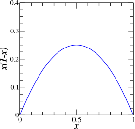
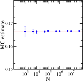
Figure 5: A simple one-dimensional Monte Carlo integration. The integrand $x(1-x)$ is shown on the left, while Monte Carlo estimates, with error bars, are shown on the right for several values of $N$, the number of random points used.

To see the method in action, consider a simple one-dimensional example:

$$\int_{0}^{1}x(1-x)\ dx=\frac{1}{6}=0.166666\cdots.$$

The integrand is plotted in Fig. 5. Various Monte Carlo estimates, including error bars, for different values of $N$, the number of random points used, are also shown in this figure. One sees the error decreasing as $N$ increases, but notice that the method is not particularly efficient in this simple case.

The Monte Carlo method works best for flat functions, and is most problematic when the integrand is sharply peaked or rapidly oscillates. Importance sampling can greatly improve the efficiency of Monte Carlo integration by dramatically reducing the variance in the estimates. Recall that a simple Monte Carlo integration is achieved by

$$\int_{a}^{b}f(x)\ dx\approx\frac{(b-a)}{N}\sum_{j=1}^{N}f(x_{j}),$$

where the $x_{j}$ are chosen with uniform probability between $a$ and $b$. Suppose that one could find a function $g(x)>0$ with $\int_{a}^{b}g(x)dx=1$ such that $h(x)=\dfrac{f(x)}{g(x)}$ is as close as possible to a constant. The integral can then be evaluated by

$$\int_{a}^{b}f(x)dx=\int_{a}^{b}h(x)g(x)dx\approx\frac{(b-a)}{N}\sum_{j=1}^{N}h(x_{j}),$$

where the $x_{j}$ are now chosen with probability density $g(x)$. Since the function $h(x)$ is fairly flat, the Monte Carlo method can do a much better job estimating the integral in this way. The function $g(x)$ accomplishes the importance sampling, causing more points to be chosen near peaked regions. Of course, one must be able to sample with probability density $g(x)$. Also, how can one find such a suitable function $g(x)$, especially for complicated multi-dimensional integrals?

Random number generators generally produce uniform deviates. To sample other probability densities, a transformation must be applied. Consider a random variable $U$ with uniform density $p_{U}(u)=1$ for $0\leq x\leq 1$, and another random variable $Y=\phi(U)$, where $\phi$ is a strictly increasing function. A strictly increasing function ensures that the inverse function is single-valued, and also ensures that if $u+du>u$, then $y+dy>y$ for $y=\phi(u)$. The probability density $p_{Y}$ associated with the random variable $Y$ can be determined using the conservation of probability:

$$p_{Y}(y)dy=p_{U}(u)du,\qquad p_{Y}(y)=p_{U}(u)\frac{du}{dy}=p_{U}(\phi^{-1}(y))\frac{d\phi^{-1}(y)}{dy}.$$

Usually the desired density $p_{Y}$ is known, so the function $\phi$ must be determined. For a uniform deviate $p_{U}(u)=1$, then $du=p_{Y}(y)dy$, and integrating yields

$$\int_{0}^{u}\!\!du^{\prime}=\int_{\phi(0)}^{\phi(u)}\!\!\!\!\!\!p_{Y}(y)\,dy\quad\Rightarrow\quad u=F_{Y}(\phi(u))\quad\Rightarrow\quad\phi(u)=F_{Y}^{-1}(u).$$

$F^{-1}$ is unique since $F$ is a strictly increasing function. In summary: a random variable $Y$ with probability density $p_{Y}(y)$ and cumulative distribution $F_{Y}(y)=\int_{-\infty}^{y}p_{Y}(s)\,ds$ can be sampled by first choosing $U$ with uniform probability in some interval, then applying the transformation

$$Y=F_{Y}^{-1}(U).$$

This transformation method is only applicable for probability densities whose indefinite integral can be obtained and inverted. Thus, the method is useful for only a handful of density functions. One such example is the exponential distribution:

$$p_{Y}(y)=\frac{e^{-y}}{1-e^{-b}},\qquad\mbox{for $0\leq y\leq b$}.$$

The cumulative distribution and its inverse are

$$F_{Y}(y) = \int_{0}^{y}p_{Y}(s)ds=\frac{(1-e^{-y})}{(1-e^{-b})},$$

$$F^{-1}_{Y}(u) = -\ln\Bigl{(}1-(1-e^{-b})u\Bigr{)}.$$

Now consider the integral

$$\int_{0}^{3}\frac{e^{-s}\ ds}{1+s/9}\approx 0.873109.$$

The integrand is shown in Fig. 6, and various Monte Carlo estimates with and without importance sampling of the integral are also shown in the figure. Estimates using importance sampling (triangles) are seen to have much smaller statistical uncertainties for a given value of $N$, the number of random points used.

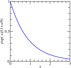
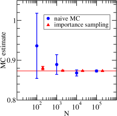
Figure 6: Plot of the integrand $e^{-s}/(1+s/9)$ on the left, and Monte Carlo estimates of the integral on the right. Circles show estimates without importance sampling, whereas triangles show estimates using importance sampling. Statistical uncertainties using importance sampling are dramatically smaller for a given value of $N$, the number of random points used.

Probability densities whose cumulative distributions are not easily calculable and invertible can be sampled using the rejection method. This method exploits the fact that sampling from a density $p_{X}(x)$ for $a\leq x\leq b$ is equivalent to choosing a random point in two dimensions with uniform probability in the area under the curve $p_{X}(x)$.

For example, one can pick a random point with uniform probability in a box $a\leq x\leq b$ horizontally and $0\leq y\leq\max(p_{X}(x))$ vertically; the result is accepted if it lies below the curve, but if above the curve, the result is rejected and the procedure repeated until an acceptance occurs. If $p_{X}(x)$ is sharply peaked, then a more efficient implementation of the method uses a comparison function $f(x)$ satisfying $f(x)\geq p_{X}(x)$ for all $a\leq x\leq b$ and which can be sampled by the transformation method.

3.3 Monte Carlo using stationary stochastic processes

The sampling methods described so far work well in one-dimension, but for multi-dimensional integrals, the transformation and rejection methods are usually not feasible. Fortunately, highly multi-dimensional integrals can be handled by exploiting stationary stochastic processes.

A stochastic process is a sequence of events $X_{t},\ t=0,1,2,\dots$ governed by probabilistic laws (we shall limit our attention to discrete “time” $t$). Consider a system which can be in one of $R$ discrete states $s_{1},s_{2},\dots,s_{R}$ (generalization to a continuum of states is usually straightforward). The system moves or steps successively from one state to another. Given previous states of the system $X_{0},X_{1},\dots,X_{t-1}$, the conditional probability to find the system in state $X_{t}$ at time $t$ is denoted by $P(X_{0},\dots,X_{t-1}|X_{t})$ and may depend on previous states of the system and possibly $t$.

A stochastic process is stationary when the probabilistic laws remain unchanged through shifts in time. In other words, the joint probability distribution of $(X_{t},X_{t+j_{1}},\dots,X_{t+j_{n}})$ is the same as that of $(X_{t+h},X_{t+h+j_{1}},\dots,X_{t+h+j_{n}})$ for any $h$. For such processes, the mean $E(X_{t})=\mu$ is independent of $t$ (if it exists) and the variance $E((X_{t}-\mu)^{2})=\sigma^{2}$ is independent of $t$ if $E(X_{t}^{2})$ is finite. However, the $X_{t}$ are usually not independent random variables, but the autocovariance $E((X_{t}-\mu)(X_{s}-\mu))=R(|t-s|)$ depends only on the time difference $|t-s|$. The autocorrelation function is defined by $\rho(t)=R(t)/R(0)$ so that $\rho(0)=1$ and $-1\leq\rho(t)\leq 1$ for all $t$ (from Schwartz’s inequality).

The Monte Carlo method described so far requires statistically independent random points. In order to use points generated by a stationary stochastic process, we must revisit the law of large numbers and the central limit theorem for the case of dependent random variables.

The law of large numbers for stationary stochastic processes: Consider a stationary stochastic process $X_{1},X_{2},\dots$ with $E(X_{k})=\mu$ and autocovariance $R(s)=E((X_{k}-\mu)(X_{k+s}-\mu))$ satisfying $\sum_{s=0}^{\infty}|R(s)|<\infty$, and define $\overline{X}_{N}=(X_{1}+X_{2}+\dots+X_{N})/N$, then

$$\lim_{N\rightarrow\infty}P(|\overline{X}_{N}-\mu|\geq\varepsilon)=0,\quad\mbox{for any $\varepsilon>0$}.$$

Proof 3.5.

Define $Y_{n}=X_{n}-\mu$ and $\overline{Y}_{N}=(Y_{1}+\dots+Y_{N})/N$, then

$$E(\overline{Y}_{N}^{2}) = \frac{1}{N^{2}}E\Bigl{(}\sum_{k=1}^{N}Y_{k}^{2}\!+\!2\sum_{k<l}Y_{k}Y_{l}\Bigr{)}=\frac{1}{N^{2}}\Bigl{(}NR(0)\!+\!2\sum_{k<l}R(l\!-\!k)\Bigr{)},$$

$$= \frac{R(0)}{N}+\frac{2}{N^{2}}\sum_{k=1}^{N-1}(N-k)\ R(k),$$

so that

$$NE(\overline{Y}_{N}^{2}) = \Bigl{|}R(0)+\textstyle\sum_{k=1}^{N-1}2R(k)(N-k)/N\Bigr{|},$$

$$\leq |R(0)|+\textstyle\sum_{k=1}^{N-1}2|R(k)|\ (N-k)/N,$$

$$\leq |R(0)|+\textstyle\sum_{k=1}^{N-1}2|R(k)|.$$

Since $\sum_{j}|R(j)|<\infty$, then $NE(\overline{Y}_{N}^{2})<\infty$ so $\lim_{N\rightarrow\infty}E(\overline{Y}_{N}^{2})=0$. The Chebyshev inequality tells us that $P(|\overline{X}_{N}-\mu|\geq\varepsilon)\leq E((\overline{X}_{N}-\mu)^{2})/\varepsilon^{2}$ so

$$\lim_{N\rightarrow\infty}E((\overline{X}_{N}-\mu)^{2})=0\ \mbox{implies}\ \lim_{N\rightarrow\infty}P(|\overline{X}_{N}-\mu|\geq\varepsilon)=0,$$

which proves the weak law of large numbers for a stationary stochastic process with an absolutely summable autocovariance.

One can show that the limiting value of the variance is

$$\lim_{N\rightarrow\infty}NE((\overline{X}_{N}-\mu)^{2})=\sum_{k=-\infty}^{\infty}R(k).$$

Proof 3.6.

Since the autocovariance is absolutely summable $\sum_{k}|R(k)|<\infty$, then for any $\varepsilon>0$ there exists a $q$ such that $\sum_{k=1}^{\infty}2|R(q+k)|<\varepsilon/2$. Hence,

$$\Bigl{|}\!\!\!\!\!\sum_{j=-(N\!-\!1)}^{N\!-\!1}\!\!\!\!\!\!R(j)\!-\!NE(\overline{Y}_{N}^{2})\Bigr{|} = \Bigl{|}R(0)\!+\!2\!\!\sum_{j=1}^{N-1}\!R(j)\!-\!\Bigl{(}\!R(0)\!+\!\sum_{k=1}^{N-1}\!\!2R(k)(N\!-\!k)/N\Bigr{)}\Bigr{|}$$

$$= \Bigl{|}\textstyle\sum_{k=1}^{N-1}2kR(k)/N\Bigr{|}\leq\sum_{k=1}^{N-1}2k|R(k)|\ /N$$

$$= \textstyle\sum_{k=1}^{q}2k|R(k)|\ /N+\sum_{k=q+1}^{N-1}2k|R(k)|\ /N$$

$$\leq \textstyle\sum_{k=1}^{q}2k|R(k)|\ /N+\sum_{k=q+1}^{N-1}2|R(k)|$$

$$\leq \textstyle\sum_{k=1}^{q}2k|R(k)|\ /N+\varepsilon/2.$$

Since $q$ fixed and finite, we can always increase $N$ so that $\sum_{k=1}^{q}2k|R(k)|\ /N<\varepsilon/2$ which holds as $N\rightarrow\infty$. Thus,

$$\Bigl{|}\!\!\!\!\!\sum_{j=-(N\!-\!1)}^{N\!-\!1}\!\!\!\!\!\!R(j)\!-\!NE(\overline{Y}_{N}^{2})\Bigr{|}<\varepsilon,$$

which proves the required result in the limit as $N\rightarrow\infty$.

The $M$-dependent central limit theorem states the following: Let $X_{1},X_{2},\dots,X_{N}$ be a stationary $M$-dependent sequence of random variables ($X_{t}$ and $X_{t+s}$ are independent for $s>M$) such that $E(X_{t})=E(X_{1})=\mu$ and $E((X_{1}\!-\!\mu)^{2})<\infty$, and define $\overline{X}_{N}=(X_{1}+X_{2}+\dots+X_{N})/N$ and $\sigma^{2}=E((X_{1}\!-\!\mu)^{2})+2\sum_{h=1}^{M}E((X_{1}\!-\!\mu)(X_{h+1}\!-\!\mu))$. Then for $a<b$,

$$\lim_{N\rightarrow\infty}P\left(\frac{a\sigma}{\sqrt{N}}<(\overline{X}_{N}-\mu)<\frac{b\sigma}{\sqrt{N}}\right)=\frac{1}{\sqrt{2\pi}}\int_{a}^{b}e^{-x^{2}/2}dx.$$

In other words, the distribution of $(X_{1}+\dots+X_{N}-N\mu)/(\sigma\sqrt{N})$ tends to a standard normal distribution (zero mean, unit variance). For the proof of this very important theorem, see Ref. Hoeffding or Ref. anderson. One version of the proof relies upon splitting the summation into blocks in such a way that the resulting variables are essentially independent. Note that

$$\sigma^{2}=\sum_{h=-M}^{M}R(h)=NE((\overline{X}_{N}-\mu)^{2})\ \ \mbox{for $N\gg M$},$$

where the autocovariance $R(h)=R(-h)=E((X_{t}\!-\!\mu)(X_{t+|h|}\!-\!\mu))$ as usual.

Monte Carlo integration using a stationary stochastic process is summarized by the following formula:

$$\displaystyle\int_{\cal V}p(\vec{x})\ f(\vec{x})\ d^{D}x\approx\langle f\rangle\pm\sqrt{\frac{R_{0}(f)+2\sum_{h\geq 1}R_{h}(f)}{N}},$$

$$\displaystyle\langle f\rangle\equiv\frac{1}{N}\!\sum_{i=1}^{N}f(\vec{x}_{i}),\quad R_{h}(f)\equiv\frac{1}{N\!-\!h}\sum_{i=1}^{N-h}\Bigl{(}f(\vec{x}_{i})\!-\!\langle f\rangle\!\Bigr{)}\Bigl{(}f(\vec{x}_{i+h})\!-\!\langle f\rangle\!\Bigr{)},$$

where the $N$ points $\vec{x}_{1},\dots,\vec{x}_{N}$ are elements of a stationary stochastic process with stationary probability distribution $p(\vec{x})$ throughout the $D$-dimensional volume ${\cal V}$, which satisfies the normalization condition $\int_{\cal V}p(\vec{x})d^{D}x=1$. One requires that the autocovariance is absolutely summable, that is, $\sum_{h=0}^{\infty}|R_{h}(f)|<\infty$. The law of large numbers justifies the correctness of the estimate, and the $M$-dependent central limit theorem gives an estimate of the statistical uncertainty.

3.4 Markov chains

Markov chains are one of the simplest types of stochastic processes. Markov chains were introduced by the Russian mathematician Andrei Markov (1856-1922) in 1906. In this section, we will discuss Markov chains in great detail.

A Markov chain is a stochastic process which generates a sequence of states with probabilities depending only on the current state of the system. Consider a system which can be in one of $R$ states $s_{1},s_{2},\dots,s_{R}$ (again, generalization to a continuum of states is usually straightforward). The system moves or steps successively from one state to another (we shall only consider discrete “time” Markov chains). If the current state is $s_{i}$, then the chain moves to state $s_{j}$ at the next step with probability $p_{ij}$ which does not depend on any previous states of the chain. The probabilities $p_{ij}$ are called the transition probabilities. The square $R\times R$ real-valued matrix $\mathbf{P}$ whose elements are $p_{ij}$ is called the transition matrix or the Markov matrix. Furthermore, we shall only deal with time homogeneous chains in which the transition probabilities $p_{ij}$ are independent of “time” or their position in chain.

Let us start with some basic properties of Markov chains.

• The transition matrix $\mathbf{P}$ has only non-negative entries $p_{ij}\geq 0$.

• Since the probability of going from $s_{i}$ to any state must be unity, then matrix elements must satisfy $\sum_{j=1}^{R}p_{ij}=1$ (rows sum to unity).

• If the columns also sum to unity, then $\mathbf{P}$ is called a doubly stochastic matrix.

• If $\mathbf{P}_{1}$ and $\mathbf{P}_{2}$ are Markov matrices, then the matrix product $\mathbf{P}_{1}\mathbf{P}_{2}$ is also a Markov matrix.

• Every eigenvalue $\lambda$ of a Markov matrix satisfies $|\lambda|\leq 1$.

• Every Markov matrix has at least one eigenvalue equal to unity.

It may be helpful at this point to review the properties of the eigenvalues and eigenvectors of real square matrices.

• For a square matrix $\mathbf{P}$, a nonzero column vector $\mathbf{v}$ which satisfies $\mathbf{P}\mathbf{v}=\lambda\mathbf{v}$ for complex scalar $\lambda$ is known as a right eigenvector corresponding to eigenvalue $\lambda$. Often, “right eigenvectors” are simply called “eigenvectors”.

• A nonzero vector $\mathbf{v}$ satisfying $\mathbf{v}^{T}\mathbf{P}=\lambda\mathbf{v}^{T}$, where $T$ indicates transpose, is known as a left eigenvector.

• Every square $R\times R$ matrix has $R$ complex eigenvalues, counting multiple roots according to their multiplicity.

• For a real square matrix, the eigenvalues are either real or come in complex conjugate pairs.

• Eigenvectors for distinct eigenvalues are linearly independent.

• A degenerate eigenvalue may not have distinct eigenvectors.

• $R$ linearly independent eigenvectors are guaranteed only if all $R$ eigenvalues are distinct.

• A matrix $\mathbf{P}$ and its transpose $\mathbf{P}^{T}$ have the same eigenvalues.

Now let us look at the last two properties of Markov matrices above in more detail.

• Every eigenvalue $\lambda$ of Markov matrix $\mathbf{P}$ satisfies $|\lambda|\leq 1$.

Proof 3.7.

Suppose that a complex number $\lambda$ is an eigenvalue of $\mathbf{P}$ with corresponding eigenvector $\mathbf{v}$ so that $\mathbf{P}\mathbf{v}=\lambda\mathbf{v}$. Let $k$ be such that $|v_{k}|\geq|v_{j}|$ for all $j$, then the $k$-th component of the eigenvalue equation gives us $\sum_{j}p_{kj}v_{j}=\lambda v_{k}$. Use the generalized triangle inequality for complex numbers $|\sum_{k}z_{k}|\leq\sum_{k}|z_{k}|$ to show

$$|\lambda v_{k}|=|\textstyle\sum_{j}p_{kj}v_{j}|\leq\sum_{j}p_{kj}|v_{j}|\leq\sum_{j}p_{kj}|v_{k}|=|v_{k}|$$

Thus, $|\lambda v_{k}|=|\lambda||v_{k}|\leq|v_{k}|$ implying $|\lambda|\leq 1$, which completes the proof.

• Every Markov matrix $\mathbf{P}$ has at least one eigenvalue equal to unity.

Proof 3.8.

Let $\mathbf{v}$ be a vector satisfying $v_{j}=1$ for all $j$, then $\sum_{j}p_{ij}v_{j}=\sum_{j}p_{ij}=1=v_{i}$. Hence, $\mathbf{v}$ is an eigenvector corresponding to eigenvalue $1$, so every Markov matrix has at least one eigenvalue equal to unity.

Multi-step probabilities are determined from powers of the Markov matrix. The $ij$-th element $p^{(n)}_{ij}$ of the matrix $\mathbf{P}^{n}$ is the probability that a Markov chain, starting in state $s_{i}$, will be in state $s_{j}$ after $n$ steps; this is usually called the $n$-step transition probability. For example, the probability to go from $s_{i}$ to $s_{j}$ in 2 steps is $\sum_{k=1}^{R}p_{ik}p_{kj}$. For a starting probability vector $\mathbf{u}$, the probability that the chain is in state $s_{j}$ after $n$ steps is $u_{j}^{(n)}=\sum_{i=1}^{R}u_{i}p^{(n)}_{ij}$. Note that $u_{i}$ is the probability that the starting state is $s_{i}$. The previous expression can be written in matrix form by $\mathbf{u}^{(n)T}=\mathbf{u}^{T}\mathbf{P}^{n}$.

Another important concept is the first visit probability, which is the probability that a Markov chain, starting in state $s_{i}$, is found for the first time in state $s_{j}$ after $n$ steps. This first visit probability is here denoted by $f_{ij}^{(n)}$. We define $f_{ij}^{(0)}=0$, and for one step, $f_{ij}^{(1)}=p_{ij}$. For two steps, $f_{ij}^{(2)}=\sum_{k\neq j}p_{ik}p_{kj}$ which generalizes to $n$-steps as

$$f_{ij}^{(n)}=\sum_{k\neq j}p_{ik}\ f_{kj}^{(n-1)}.$$

An important relation for later use is

$$p_{ij}^{(n)}=\displaystyle\sum_{m=1}^{n}f_{ij}^{(m)}p_{jj}^{(n-m)}.$$

The total visit probability $f_{ij}$ is the probability that, starting from state $s_{i}$, the chain will ever visit state $s_{j}$:

$$f_{ij}=\sum_{n=1}^{\infty}f_{ij}^{(n)}.$$

The mean first passage time $m_{ij}$ from $s_{i}$ to $s_{j}$ is the expected number of steps to reach state $s_{j}$ in a Markov chain for the first time, starting from state $s_{i}$ (by convention, $m_{ii}=0$):

$$m_{ij}=\sum_{n=1}^{\infty}n\ f_{ij}^{(n)}.$$

The mean recurrence time $\mu_{i}$ of state $s_{i}$ is the expected number of steps to return to state $s_{i}$ for the first time in a Markov chain starting from $s_{i}$:

$$\mu_{i}=\sum_{n=1}^{\infty}n\ f_{ii}^{(n)}.$$

Classes are an important concept in studying Markov chains. State $s_{j}$ is called accessible from state $s_{i}$ if $p_{ij}^{(n)}>0$ for some finite $n$. This is often denoted by $s_{i}\rightarrow s_{j}$. Note that if $s_{i}\rightarrow s_{j}$ and $s_{j}\rightarrow s_{k}$, then $s_{i}\rightarrow s_{k}$. States $s_{i}$ and $s_{j}$ are said to communicate if $s_{i}\rightarrow s_{j}$ and $s_{j}\rightarrow s_{i}$; this is denoted by $s_{i}\leftrightarrow s_{j}$. Note that $s_{i}\leftrightarrow s_{j}$ and $s_{j}\leftrightarrow s_{k}$ implies $s_{i}\leftrightarrow s_{k}$. A class is a set of states that all communicate with one another. If $C_{1}$ and $C_{2}$ are communicating classes, then either $C_{1}=C_{2}$ or $C_{1}$ and $C_{2}$ are disjoint. To see this, start by noting that if $C_{1}$ and $C_{2}$ have a common state $s_{i}$, then $s_{i}\leftrightarrow s_{j1}$ for all $s_{j1}\in C_{1}$ and $s_{i}\leftrightarrow s_{j2}$ for all $s_{j2}\in C_{2}$, so $s_{j1}\leftrightarrow s_{j2}$, implying $C_{1}=C_{2}$. This means that the set of all states can be partitioned into separate non-intersecting classes. Also, if a transition from class $C_{1}$ to a different class $C_{2}$ is possible, then a transition from $C_{2}$ to $C_{1}$ must not be possible, since this would imply $C_{1}=C_{2}$.

A Markov chain is called irreducible if the probability to go from every state to every state (not necessarily in one step) is greater than zero. All states in an irreducible chain are in one single communicating class.

States in a Markov chain can be classified according to whether they are (a) positive recurrent (persistent), (b) null recurrent, or (c) transient. A recurrent or persistent state has $f_{ii}=\sum_{n=1}^{\infty}f_{ii}^{(n)}=1$, that is, there is unit probability of returning to the state after a finite length of time in the chain. A transient state has $f_{ii}=\sum_{n=1}^{\infty}f_{ii}^{(n)}<1$. A recurrent state is positive if its mean recurrence time is finite $\mu_{i}<\infty$; otherwise, it is called null.

In addition, states in a Markov chain can be classified according to whether they are periodic (cyclic) or aperiodic. The period of a state in a Markov chain is the greatest common divisor of all $n\geq 0$ for which $p^{(n)}_{ii}>0$. In other words, the transition $s_{i}$ to $s_{i}$ is not possible except for time intervals which are multiples of the period $d(i)$. A periodic state $s_{i}$ has period $d(i)>1$, whereas an aperiodic state $s_{i}$ has period $d(i)=1$.

For a recurrent state, $\sum_{n=1}^{\infty}p^{(n)}_{ii}=\infty$, whereas for a transient state, $\sum_{n=1}^{\infty}p^{(n)}_{ii}<\infty$.

Proof 3.9.

Start with the following:

$$\sum_{n=1}^{N}p_{ij}^{(n)}=\sum_{n=1}^{N}\sum_{m=1}^{n}f_{ij}^{(m)}p_{jj}^{(n-m)}=\sum_{m=1}^{N}f_{ij}^{(m)}\sum_{n=0}^{N-m}p_{jj}^{(n)}\leq\sum_{m=1}^{N}f_{ij}^{(m)}\sum_{n=0}^{N}p_{jj}^{(n)},$$

since $p_{jj}^{(n)}\geq 0$, but for $N>N^{\prime}$, we also have

$$\sum_{n=1}^{N}p_{ij}^{(n)}=\sum_{m=1}^{N}f_{ij}^{(m)}\sum_{n=0}^{N-m}p_{jj}^{(n)}\geq\sum_{m=1}^{N^{\prime}}f_{ij}^{(m)}\sum_{n=0}^{N-m}p_{jj}^{(n)}\geq\sum_{m=1}^{N^{\prime}}f_{ij}^{(m)}\sum_{n=0}^{N-N^{\prime}}p_{jj}^{(n)},$$

again since the $p_{jj}^{(n)}\geq 0$ and $f_{ij}^{(m)}\geq 0$. Putting together the above results yields

$$\sum_{m=1}^{N^{\prime}}f_{ij}^{(m)}\sum_{n=0}^{N-N^{\prime}}p_{jj}^{(n)}\leq\sum_{n=1}^{N}p_{ij}^{(n)}\leq\sum_{m=1}^{N}f_{ij}^{(m)}\sum_{n=0}^{N}p_{jj}^{(n)}.$$

Take $N\rightarrow\infty$ first, then $N^{\prime}\rightarrow\infty$ to get

$$f_{ij}\sum_{n=0}^{\infty}p_{jj}^{(n)}\leq\sum_{n=1}^{\infty}p_{ij}^{(n)}\leq f_{ij}\sum_{n=0}^{\infty}p_{jj}^{(n)}\quad\Rightarrow\quad f_{ij}\sum_{n=0}^{\infty}p_{jj}^{(n)}=\sum_{n=1}^{\infty}p_{ij}^{(n)}.$$

Set $i=j$ and use $p_{jj}^{(0)}=1$ to see that $f_{ii}(1+\sum_{n=1}^{\infty}p_{ii}^{(n)})=\sum_{n=1}^{\infty}p_{ii}^{(n)}$, so

$$\sum_{n=1}^{\infty}p_{ii}^{(n)}=\frac{f_{ii}}{1-f_{ii}}.$$

Now use the facts that $f_{ii}=1$ for a recurrent state and $f_{ii}<1$ for a transient state to complete the proof of the above statements.

Note that the above results also imply

$$\sum_{n=1}^{\infty}p_{ij}^{(n)}=\frac{f_{ij}}{1-f_{ii}}.$$

A Markov chain returns to a recurrent state infinitely often and returns to a transient state only a finite number of times.

Proof 3.10.

Let $g_{ij}(m)$ denote the probability that a Markov chain enters state $s_{j}$ at least $m$ times, starting from $s_{i}$. Clearly $g_{ij}(1)=f_{ij}$. One also sees that $g_{ij}(m+1)=f_{ij}g_{jj}(m)$, so $g_{ij}(m)=\left(f_{ij}\right)^{m}$. The probability of entering $s_{j}$ infinitely many times is $g_{ij}=\lim_{m\rightarrow\infty}g_{ij}(m)=\lim_{m\rightarrow\infty}(f_{ij})^{m}$, so starting in $s_{j}$, then

$$g_{jj}=\lim_{m\rightarrow\infty}(f_{jj})^{m}=\left\{\begin{array}[]{l@{\hspace{4mm}}l}1,\hfil\hskip 11.38109pt&\mbox{for recurrent state since $f_{jj}=1$,}\\ 0,\hfil\hskip 11.38109pt&\mbox{for transient state since $f_{jj}<1$,}\end{array}\right.$$

which completes the proof.

Another important result for recurrent states is as follows: if $s_{i}$ is recurrent and $s_{i}\rightarrow s_{j}$, then $f_{ji}=1$.

Proof 3.11.

Let $\alpha$ denote the probability to reach $s_{j}$ from $s_{i}$ without previously returning to $s_{i}$, and since $s_{i}\rightarrow s_{j}$ we know that $\alpha>0$. The probability of never returning to $s_{i}$ from $s_{j}$ is $1-f_{ji}$, and the probability of never returning to $s_{i}$ from $s_{i}$ is at least $\alpha(1-f_{ji})$. But $s_{i}$ is recurrent so the probability of no return is zero; thus, $f_{ji}=1$. For two communicating states $s_{i}\leftrightarrow s_{j}$ that are each recurrent, it follows that $f_{ij}=f_{ji}=1$.

All states in a class of a Markov chain are of the same type, and if periodic, all have the same period.

Proof 3.12.

For any two states $s_{i}$ and $s_{j}$ in a class, there exists integers $r$ and $s$ such that $p^{(r)}_{ij}=\alpha>0$ and $p_{ji}^{(s)}=\beta>0$ so

$$p_{ii}^{(n+r+s)}=\sum_{kl}p^{(r)}_{ik}p^{(n)}_{kl}p_{li}^{(s)}\geq\sum_{k}p^{(r)}_{ik}p^{(n)}_{kk}p_{ki}^{(s)}\geq p^{(r)}_{ij}p^{(n)}_{jj}p_{ji}^{(s)}=\alpha\beta p^{(n)}_{jj}.$$

If $s_{i}$ is transient, then the left-hand side is a term of a convergent series $\sum_{k}p_{ii}^{(k)}<\infty$, so the same must be true for $p_{jj}^{(k)}$, and if $p_{ii}^{(k)}\rightarrow 0$, then $p_{jj}^{(k)}\rightarrow 0$. The same statements remain true if the roles of $i$ and $j$ are reversed, so either both $s_{i}$ and $s_{j}$ are transient, or neither is. If $s_{j}$ is null (infinite mean recurrence time $\mu_{j}=\sum_{n=1}^{\infty}n\ f_{jj}^{(n)}=\infty$), then $s_{i}$ must be null as well. The same statements are true if $i,j$ are reversed, so if one is a null state, then so is the other. Similarly, we can also conclude that if either $s_{i}$ or $s_{j}$ is positive recurrent (finite mean recurrence time), then so is the other. Thus, we have shown that all states in a class are of the same type (positive recurrent, null recurrent, or transient).

Suppose $s_{i}$ has period $t$, then for $n=0$, the right-hand side of the above equation is positive, so $p_{ii}^{(r+s)}>0$, which means that $r+s$ must be a multiple of $t$. Hence, the left-hand side vanishes unless $n$ is multiple of $t$, so $p_{jj}^{(n)}$ can be nonzero only if $n$ is multiple of $t$, which means that $s_{i}$ and $s_{j}$ have the same period. Note that the chain is aperiodic if $p_{ii}>0$ for at least one $s_{i}$.

States in an irreducible chain with period $d$ can be partitioned into $d$ mutually exclusive subsets $G_{0},\cdots,G_{d-1}$ such that if state $s_{k}\in G_{\alpha}$, then $p_{1k}^{(n)}=0$ unless $n=\alpha+\nu d$.

Proof 3.13.

Since irreducible, all states have the same period $d$ and every state can be reached from every other state. There exist for every state $s_{k}$ two integers $a$ and $b$ such that $p_{1k}^{(a)}>0$ and $p_{k1}^{(b)}>0$, but $p_{11}^{(a+b)}=\sum_{j}p_{1j}^{(a)}p_{j1}^{(b)}\geq p_{1k}^{(a)}p_{k1}^{(b)}>0$, so $a+b$ divisible by $d$. Thus, $a+b=md$ for integer $m$, or $a=-b+md$. Rewrite this as $a=\alpha+\nu d$ for integer $\nu$ and $0\leq\alpha<d$. The parameter $\alpha$ is characteristic of state $s_{k}$ so all states are partitioned into $d$ mutually exclusive subsets $G_{0},G_{1},\cdots,G_{d-1}$.

With proper ordering of the $G_{\alpha}$ subsets, a one-step transition from a state in $G_{\alpha}$ always leads to a state in $G_{\alpha+1}$, or from $G_{d-1}$ to $G_{0}$. Each subset $G_{\alpha}$ can be considered states in an aperiodic Markov chain with transition matrix $\mathbf{P}^{d}$.

As an aside, consider the following fact concerning finite Markov chains: in an irreducible chain having a finite number $R$ of states, there are no null states and it is impossible that all states are transient.

Proof 3.14.

All rows of the matrix $\mathbf{P}^{n}$ must add to unity. Since each row contains a finite number of non-negative elements, it is impossible that $p_{ij}^{(n)}\rightarrow 0$ for all $i,j$ pairs. Thus, it is impossible that all states are transient, so at least one state must be non-null. But since the chain is irreducible (one class), all states must be non-null.

In fact, in an $R$-state irreducible Markov chain, it is possible to go from any state to any other state in at most $R-1$ steps.

We now need to consider a very important theorem (often referred to as the basic limit theorem of the renewal equation) about two sequences. Given a sequence $f_{0},f_{1},f_{2},\dots$ such that

$$f_{0}=0,\qquad 0\leq f_{n}\leq 1,\qquad\sum_{n=0}^{\infty}f_{n}=1,$$

and greatest common divisor of those $n$ for which $f_{n}>0$ is $d\geq 1$, and another sequence $u_{0},u_{1},u_{2},\dots$ defined by

$$u_{0}=1,\qquad u_{n}=\sum_{m=1}^{n}f_{m}u_{n-m},\qquad(n\geq 1),$$

then

$$\lim_{n\rightarrow\infty}u_{nd}=\left\{\begin{array}[]{l@{\hspace{5mm}}l}d\mu^{-1}\hfil\hskip 14.22636pt&\mbox{if $\displaystyle\mu=\sum_{n=1}^{\infty}nf_{n}<\infty$,}\\[5.0pt] 0\hfil\hskip 14.22636pt&\mbox{if $\mu=\infty$.}\end{array}\right.$$

Proof 3.15.

See Refs. feller, karlin for a complete proof. Here, we shall only provide a sketch of the proof of this theorem. First, note some key properties of these sequences. We know that $0\leq f_{n}\leq 1$ for all $n$ since $f_{n}\geq 0$ and $\sum_{n=0}^{\infty}f_{n}=1$. Also, $0\leq u_{n}\leq 1$ for all $n$ can be established inductively. To do this, first note that $u_{0}=1,\ u_{1}=f_{1},\ u_{2}=f_{2}+f_{1}^{2}$ satisfy the above bounds. Assume $0\leq u_{k}\leq 1$ for all $0\leq k\leq n$. Since $f_{m}\geq 0$ and $\sum_{m=1}^{\infty}f_{m}=1$, then $u_{n+1}=\sum_{m=1}^{n+1}f_{m}u_{n+1-m}\geq 0$ since it is a sum of nonnegative terms, and $u_{n+1}=\sum_{m=1}^{n+1}f_{m}u_{n+1-m}\leq\sum_{m=1}^{n+1}f_{m}\leq 1$, which completes the induction.

Next, limit our attention to $d=1$ (the nonperiodic case). Since $u_{n}$ is a bounded sequence, $\lambda\equiv\limsup_{n\rightarrow\infty}u_{n}$ is finite, and there exists a subsequence $n_{1}<n_{2}<\cdots$ tending to infinity such that $\lim_{j\rightarrow\infty}u_{n_{j}}=\lambda$. The next step in the proof is to show that $\lim_{j\rightarrow\infty}u_{n_{j}-q}=\lambda$ for any integer $q\geq 0$ when $f_{1}>0$ (we skip this here).

Now define a new sequence $r_{n}=\sum_{k>n}f_{k}$. Some important properties of this sequence are $r_{n}\geq 0$ for all $n$, $r_{0}=1$, $r_{n-1}-r_{n}=f_{n}$ for $n\geq 1$, and $\sum_{n=0}^{\infty}r_{n}=\sum_{n=1}^{\infty}nf_{n}\equiv\mu$. One very crucial identity is

$$\sum_{k=0}^{N}r_{k}u_{N-k}=1,\qquad\mbox{for all $N\geq 0$}.$$

To see this, define $A_{N}=\sum_{k=0}^{N}r_{k}u_{N-k}$. Start with

$$u_{N}=\sum_{m=1}^{N}f_{m}u_{N-m}=\sum_{m=1}^{N}(r_{m-1}-r_{m})u_{N-m},$$

use $r_{0}=1$, and rearrange to get

$$r_{0}u_{N}+\sum_{m=1}^{N}r_{m}u_{N-m}=\sum_{m=1}^{N}r_{m-1}u_{N-m}.$$

Take $m\rightarrow k+1$ on the right:

$$\sum_{m=0}^{N}r_{m}u_{N-m}=\sum_{k=0}^{N-1}r_{k}u_{N-1-k},$$

which shows $A_{N}=A_{N-1}$ for all $N$. Thus, $A_{N}=A_{N-1}=A_{N-2}=\cdots=A_{0}=r_{0}u_{0}=1$.

Recall that $n_{1}<n_{2}<\cdots$ is a subsequence such that $\lim_{j\rightarrow\infty}u_{n_{j}-q}=\lambda$ for any integer $q\geq 0$. Since $\sum_{k=0}^{n_{j}}r_{k}u_{n_{j}-k}=1$ for all $n_{j}$ and $r_{k}\geq 0,\ u_{k}\geq 0$ for all $k$, then $\sum_{k=0}^{N}r_{k}u_{n_{j}-k}\leq 1$ for fixed $N<n_{j}$. Take the limit $j\rightarrow\infty$ so

$$\lim_{j\rightarrow\infty}\sum_{k=0}^{N}r_{k}u_{n_{j}-k}=\lambda\sum_{k=0}^{N}r_{k}\leq 1.$$

We already know that $\lambda\geq 0$, so take $N\rightarrow\infty$ to have

$$0\leq\lambda\leq 1/(\sum_{k=0}^{\infty}r_{k}).$$

If $\sum_{k=0}^{\infty}r_{k}=\infty$ then $\lim_{n\rightarrow\infty}u_{n}=\lambda=0$. If $\mu=\sum_{k=0}^{\infty}r_{k}$ is finite, $N\rightarrow\infty$ gives $\mu\lambda\leq 1$. Define $M=\sup_{n\geq 0}u_{n}$ so $0\leq u_{k}\leq M\leq 1$ for all $k$, and define $g(D)=\sum_{k=D+1}^{\infty}r_{k}$, noting that $g(D)\geq 0$ for all $D$ and $\lim_{D\rightarrow\infty}g(D)=0$. Consider

$$\sum_{k=0}^{D}r_{k}u_{n_{j}-k}+\sum_{k=D+1}^{n_{j}}r_{k}u_{n_{j}-k}=1,\quad\mbox{for $D<n_{j}$}.$$

Thus

$$\sum_{k=0}^{D}r_{k}u_{n_{j}-k}+Mg(D)\geq 1\quad\mbox{for $D<n_{j}$}.$$

Take $j\rightarrow\infty$ to conclude

$$\lambda\left(\sum_{k=0}^{D}r_{k}\right)+Mg(D)\geq 1.$$

Take the limit $D\rightarrow\infty$ to obtain $\lambda\mu\geq 1$. We have now shown $1\leq\mu\lambda\leq 1$ so $\mu\lambda=1$. The proof for the nonperiodic $(d=1)$ case is now complete.

When $d>1$, we know $f_{m}=0$ unless $m=nd$ for integer $n$. One can then show $u_{m}=0$ unless $m=nd$. Define new sequences $f^{\prime}_{n}=f_{nd}$ and $u^{\prime}_{n}=u_{nd}$ for $n=0,1,2,\dots$. Since the new sequence is aperiodic, we know $\lim_{n\rightarrow\infty}u^{\prime}_{n}=1/\mu^{\prime}$ where $\mu^{\prime}=\sum_{n=0}^{\infty}nf^{\prime}_{n}$. Since $f_{m}=0$ when $m\neq nd$, then

$$\mu^{\prime}=\sum_{n=0}^{\infty}nf_{nd}=d^{-1}\sum_{m=0}^{\infty}mf_{m}=\mu/d.$$

Thus, $\lim_{n\rightarrow\infty}u_{nd}=d\mu^{-1}$ as required.

An important feature of a Markov chain is the asymptotic behavior of its $n$-step probabilities as $n$ becomes large. First, consider $p_{jj}^{(n)}$, the $n$-step probability to go from state $s_{j}$ back to $s_{j}$ as $n$ becomes large. This behavior can be summarized as

$$\lim_{n\rightarrow\infty}p_{jj}^{(dn)}=\left\{\begin{array}[]{l@{\hspace{5mm}}l}0,\hfil\hskip 14.22636pt&\mbox{$s_{j}$ transient or null recurrent,}\\ \mu_{j}^{-1},\hfil\hskip 14.22636pt&\mbox{$s_{j}$ aperiodic positive recurrent,}\\ d\mu_{j}^{-1},\hfil\hskip 14.22636pt&\mbox{$s_{j}$ positive recurrent with period $d$.}\end{array}\right.$$

Proof 3.16.

If $s_{j}$ is transient, then $\sum_{n}p_{jj}^{(n)}$ is finite (converges), requiring $p_{jj}^{(n)}\rightarrow 0$. For a recurrent $s_{j}$, let $f_{n}=f_{jj}^{(n)}$ and $u_{n}=p_{jj}^{(n)}$. The sequences $f_{n},u_{n}$ so defined satisfy the conditions of the basic limit theorem of the renewal equation previously discussed, which tells us that $p_{jj}^{(dn)}\rightarrow d\mu_{j}^{-1}$ where $\mu_{j}=\sum_{n}nf_{jj}^{(n)}$ is the mean recurrence time. Of course, the aperiodic case applies when $d=1$. If $s_{j}$ is null recurrent, then $\mu_{j}=\infty$ so $p_{jj}^{(n)}\rightarrow\mu_{j}^{-1}=0$.

Next, the asymptotic behavior of $p_{ij}^{(n)}$ can be summarized as

$$\lim_{n\rightarrow\infty}p_{ij}^{(n)}=\left\{\begin{array}[]{l@{\hspace{5mm}}l}0,\hfil\hskip 14.22636pt&\mbox{$s_{j}$ transient or null recurrent,}\\ f_{ij}\mu_{j}^{-1},\hfil\hskip 14.22636pt&\mbox{$s_{j}$ aperiodic positive recurrent.}\end{array}\right.$$

Here, we will ignore the periodic case.

Proof 3.17.

Start by noting that

$$p_{ij}^{(n)}=\sum_{m=1}^{n}f_{ij}^{(m)}p_{jj}^{(n-m)}=\sum_{m=1}^{n^{\prime}}f_{ij}^{(m)}p_{jj}^{(n-m)}\!\!+\!\!\sum_{m=n^{\prime}+1}^{n}f_{ij}^{(m)}p_{jj}^{(n-m)}\quad(n^{\prime}<n).$$

Since $0\leq\sum_{m=n^{\prime}+1}^{n}f_{ij}^{(m)}p_{jj}^{(n-m)}\leq\sum_{m=n^{\prime}+1}^{n}f_{ij}^{(m)}$, then

$$\textstyle 0\leq\Bigl{(}p_{ij}^{(n)}-\sum_{m=1}^{n^{\prime}}f_{ij}^{(m)}p_{jj}^{(n-m)}\Bigr{)}\leq\sum_{m=n^{\prime}+1}^{n}f_{ij}^{(m)}\quad(n^{\prime}<n).$$

Take $n\rightarrow\infty$, then $n^{\prime}\rightarrow\infty$ above, and denote $p_{jj}=\lim_{n\rightarrow\infty}p_{jj}^{(n)}$ to deduce

$$\textstyle 0\leq\Bigl{(}\lim_{n\rightarrow\infty}p_{ij}^{(n)}-p_{jj}f_{ij}\Bigr{)}\leq 0\quad\Rightarrow\quad\lim_{n\rightarrow\infty}p_{ij}^{(n)}=p_{jj}\,f_{ij}.$$

For the case of $s_{j}$ transient or null recurrent, $p_{jj}=0$ and $f_{ij}$ finite, so $\lim_{n\rightarrow\infty}p_{ij}^{(n)}=0$. For $s_{j}$ aperiod and positive recurrent, $p_{jj}=\mu_{j}^{-1}$ so $p_{ij}^{(n)}\rightarrow f_{ij}\mu_{j}^{-1}$.

The above information will be needed in proving a very important property of irreducible aperiodic Markov chains. Before getting to this property, it is convenient to introduce a few definitions and remind the reader of two lemmas concerning sequences.

A probability vector $\mathbf{w}$ is called stationary or invariant or a fixed-point if $\mathbf{w}^{T}=\mathbf{w}^{T}\mathbf{P}$. Clearly, one also has $\mathbf{w}^{T}=\mathbf{w}^{T}\mathbf{P}^{n}$. If one starts a Markov chain with an initial probability vector that is stationary, then the probability vector is always the same (stationary) for the chain. When this occurs, the Markov chain is said to be in equilibrium.

Fatou’s lemma and the dominated convergence theorem will be needed in demonstrating an important property of Markov chains, so these theorems are briefly recapped next.

Fatou’s lemma: Let $a_{n}(t)$ for $n=1,2,\dots$ be a function on a discrete set $T=\{1,2,\dots\}$, assume $\lim_{n\rightarrow\infty}a_{n}(t)$ exists for each $t$ in $T$, and suppose $a_{n}(t)\geq 0$ for all $t,n$, then

$$\sum_{t\in T}\left(\lim_{n\rightarrow\infty}a_{n}(t)\right)\leq\lim_{n\rightarrow\infty}\sum_{t\in T}a_{n}(t).$$

Proof 3.18.

For any integer $M$

$$\sum_{t=1}^{M}\left(\lim_{n\rightarrow\infty}a_{n}(t)\right)=\lim_{n\rightarrow\infty}\sum_{t=1}^{M}a_{n}(t)\leq\lim_{n\rightarrow\infty}\sum_{t=1}^{\infty}a_{n}(t),$$

since all $a_{n}(t)\geq 0$. Take the limit $M\rightarrow\infty$ to obtain required result.

This lemma shows that taking the limit then summing the sequence is not the same as summing the sequence, then taking the limit. For example, consider $a_{n}(t)=n/(n^{2}+t^{2})$. For $n>t$ then $\lim_{n\rightarrow\infty}a_{n}(t)=0$ so $\sum_{t=1}^{\infty}\left(\lim_{n\rightarrow\infty}a_{n}(t)\right)=0$. But

$$\sum_{t=1}^{\infty}a_{n}(t)=\frac{\pi}{2}\coth(n\pi)-\frac{1}{2n}\quad\mbox{so}\quad\lim_{n\rightarrow\infty}\sum_{t=1}^{\infty}a_{n}(t)=\frac{\pi}{2}.$$

The dominated convergence theorem: Let $a_{n}(t)$ for $n=1,2,\dots$ be a function on a discrete set $T=\{1,2,\dots\}$, assume $\lim_{n\rightarrow\infty}a_{n}(t)$ exists for each $t$ in $T$, and suppose a function $B(t)$ exists such that $|a_{n}(t)|\leq B(t)$ for all $t,n$ and $\sum_{t\in T}B(t)<\infty$, then

$$\sum_{t\in T}\left(\lim_{n\rightarrow\infty}a_{n}(t)\right)=\lim_{n\rightarrow\infty}\sum_{t\in T}a_{n}(t).$$

Proof 3.19.

Let $a(t)\!=\!\displaystyle\lim_{n\rightarrow\infty}a_{n}(t)$ and given $|a(t)|\leq B(t)$, then $\sum_{t=1}^{\infty}a(t)$ converges since $\sum_{t=1}^{\infty}B(t)$ converges. For any integer $M$,

$$\Bigl{|}\sum_{t=1}^{\infty}a_{n}(t)-\sum_{t=1}^{\infty}a(t)\Bigr{|}\leq\sum_{t=1}^{M}|a_{n}(t)-a(t)|\!+\!\sum_{t=M+1}^{\infty}\Bigl{(}|a_{n}(t)|+|a(t)|\Bigr{)}.$$

Next, take the limit $n\rightarrow\infty$, and for a finite sum of positive terms, the summation and limit can be taken in any order:

$$\lim_{n\rightarrow\infty}\sum_{t=1}^{M}|a_{n}(t)\!-\!a(t)|=\sum_{t=1}^{M}\Bigl{(}\lim_{n\rightarrow\infty}|a_{n}(t)\!-\!a(t)|\Bigr{)}=0.$$

We also have

$$\sum_{t=M+1}^{\infty}\Bigl{(}|a_{n}(t)|\!+\!|a(t)|\Bigr{)}\leq 2\sum_{t=M+1}^{\infty}B(t),$$

so for any integer $M$,

$$\Bigl{|}\lim_{n\rightarrow\infty}\sum_{t=1}^{\infty}a_{n}(t)-\sum_{t=1}^{\infty}\lim_{n\rightarrow\infty}a_{n}(t)\Bigr{|}\leq 2\sum_{t=M+1}^{\infty}B(t).$$

The right-hand side is the remainder of a convergent series, which means that it must equal zero in the $M\rightarrow\infty$ limit. The equality to be shown easily follows.

The dominated convergence theorem essentially specifies the conditions under which the order of taking an asymptotic limit and summing a sequence does not matter.

And now, without further adieu, we state the very important fundamental limit theorem for irreducible Markov chains: An irreducible aperiodic Markov chain with transition matrix $\mathbf{P}$ has a stationary distribution $\mathbf{w}$ satisfying $w_{j}>0$, $\sum_{j}w_{j}=1$, and $\mathbf{w}^{T}=\mathbf{w}^{T}\mathbf{P}$ if, and only if, all its states are positive recurrent, and this stationary distribution is unique and identical to the limiting distribution $w_{j}=\lim_{n\rightarrow\infty}p_{ij}^{(n)}$ independent of initial state $s_{i}$.

Proof 3.20.

For an irreducible aperiodic chain, the following possibilities exist:
     (a) all states are positive recurrent (an ergodic chain),
     (b) all states are null recurrent,
     (c) all states are transient.
If all states are transient or null recurrent, then $\lim_{n\rightarrow\infty}p_{ij}^{(n)}=0$. If all states are positive recurrent, then since all states communicate, $f_{ij}=1$ for all $i,j$ and the basic limit theorem of the renewal equation tells us that $\lim_{n\rightarrow\infty}p_{ij}^{(n)}=\mu_{j}^{-1}$. Let us define $w_{j}=\lim_{n\rightarrow\infty}p_{ij}^{(n)}=\mu_{j}^{-1}$ which is independent of the initial state $s_{i}$. For all states positive recurrent, then $0<\mu_{j}<\infty$ so $w_{j}>0$ for all $j$. We have $p_{ij}^{(m+n)}=\sum_{k=1}^{\infty}p_{ik}^{(n)}p_{kj}^{(m)}$ so using Fatou’s lemma:

$$\lim_{n\rightarrow\infty}p_{ij}^{(m+n)}=\lim_{n\rightarrow\infty}\sum_{k=1}^{\infty}p_{ik}^{(n)}p_{kj}^{(m)}\geq\sum_{k=1}^{\infty}\lim_{n\rightarrow\infty}p_{ik}^{(n)}p_{kj}^{(m)}.$$

Taking the limit $n\rightarrow\infty$ yields $w_{j}\geq\sum_{k=1}^{\infty}w_{k}\ p^{(m)}_{kj}$. Define $s\equiv\sum_{k=1}^{\infty}w_{k}$, then sum the above equation over $j$:

$$s=\sum_{j=1}^{\infty}w_{j}\geq\sum_{j=1}^{\infty}\sum_{k=1}^{\infty}w_{k}\ p^{(m)}_{kj}=\sum_{k=1}^{\infty}w_{k}\sum_{j=1}^{\infty}p^{(m)}_{kj}=\sum_{k=1}^{\infty}w_{k}=s,$$

where we used the fact that the rows of the Markov matrix and its powers sum to unity. Interchanging the order of the two infinite summations above is possible since all summands are non-negative (Fubini’s theorem). We have shown that $s\geq s$, which means that the equality must hold:

$$\sum_{j=1}^{\infty}w_{j}=\sum_{j=1}^{\infty}\sum_{k=1}^{\infty}w_{k}\ p_{kj}^{(m)}.$$

But for each term, we have already shown that $w_{j}\geq\sum_{k=1}^{\infty}w_{k}\ p^{(m)}_{kj}$. Since each one of the terms in the summation is known to be greater than or equal to zero, we must conclude that the equality holds term by term for every $j$:

$$w_{j}=\sum_{k=1}^{\infty}w_{k}\ p_{kj}^{(m)}.$$

For $m=1$, we see that the limiting vector $\mathbf{w}$ satisfies the criteria for a stationary vector. Next, use $\sum_{j=1}^{\infty}p_{ij}^{(n)}=1$ and Fatou’s lemma to show that

$$1=\lim_{n\rightarrow\infty}\sum_{j=1}^{\infty}p_{ij}^{(n)}\geq\sum_{j=1}^{\infty}\lim_{n\rightarrow\infty}p_{ij}^{(n)}=\sum_{j=1}^{\infty}w_{j}.$$

Given $\sum_{j}w_{j}\leq 1$, then consider the limit $m\rightarrow\infty$ of

$$w_{j}=\lim_{m\rightarrow\infty}\sum_{k=1}^{\infty}w_{k}\ p_{kj}^{(m)}.$$

Since $0\leq p_{kj}^{(m)}\leq 1$, then $|w_{k}p_{kj}^{(m)}|\leq w_{k}$ and $\sum_{k=1}^{\infty}w_{k}<\infty$ so the dominated convergence theorem can be applied:

$$w_{j}=\lim_{m\rightarrow\infty}\sum_{k=1}^{\infty}w_{k}\ p_{kj}^{(m)}=\sum_{k=1}^{\infty}w_{k}\lim_{m\rightarrow\infty}p_{kj}^{(m)}=\Bigl{(}\sum_{k=1}^{\infty}w_{k}\Bigr{)}w_{j}.$$

We can at last conclude that $\sum_{j=1}^{\infty}w_{j}=1$.

Only the uniqueness of the stationary state is left to show. If another stationary vector $\mathbf{v}$ existed, it would have to satisfy $v_{j}>0$, $\sum_{j=1}^{\infty}v_{j}=1$, and $v_{j}=\sum_{i=1}^{\infty}v_{i}p_{ij}^{(n)}$. Conditions for the dominated convergence theorem again apply, so taking the $n\rightarrow\infty$ limit gives

$$v_{j}=\lim_{n\rightarrow\infty}\sum_{i=1}^{\infty}v_{i}p_{ij}^{(n)}=\sum_{i=1}^{\infty}v_{i}\lim_{n\rightarrow\infty}p_{ij}^{(n)}=\Bigl{(}\sum_{i=1}^{\infty}v_{i}\Bigr{)}w_{j}=w_{j}.$$

Since $\mathbf{v}=\mathbf{w}$, then $\mathbf{w}$ is unique.

A simple example may help to understand the above result. Consider the following transition matrix

$$\mathbf{P}=\left[\begin{array}[]{ccc}\frac{3}{4}&\frac{1}{4}&0\\[4.0pt] 0&\frac{2}{3}&\frac{1}{3}\\[4.0pt] \frac{1}{4}&\frac{1}{4}&\frac{1}{2}\end{array}\right].$$

Since $\mathbf{P}^{2}$ has all positive entries (greater than zero), this Markov chain is irreducible. The eigenvalues of $\mathbf{P}$ are $1,\frac{1}{2},\frac{5}{12}$, and the unnormalized right and left eigenvectors are

$$\mbox{right:}\begin{array}[]{c}1\\[6.0pt] \left[\begin{array}[]{r}1\\ 1\\ 1\end{array}\right]\end{array}\begin{array}[]{c}\frac{1}{2}\\[6.0pt] \left[\begin{array}[]{r}2\\ -2\\ 1\end{array}\right]\end{array}\begin{array}[]{c}\frac{5}{12}\\[6.0pt] \left[\begin{array}[]{r}3\\ -4\\ 3\end{array}\right]\end{array}\qquad\mbox{left:}\begin{array}[]{c}1\\[6.0pt] \left[\begin{array}[]{r}2\\ 3\\ 2\end{array}\right]\end{array}\begin{array}[]{c}\frac{1}{2}\\[6.0pt] \left[\begin{array}[]{r}-1\\ 0\\ 1\end{array}\right]\end{array}\begin{array}[]{c}\frac{5}{12}\\[6.0pt] \left[\begin{array}[]{r}-3\\ -1\\ 4\end{array}\right]\end{array}.$$

The left fixed-point probability vector and $\lim_{n\rightarrow\infty}\mathbf{P}^{n}$ are

$$\mathbf{w}=\frac{1}{7}\left[\begin{array}[]{r}2\\ 3\\ 2\end{array}\right],\quad\lim_{n\rightarrow\infty}\mathbf{P}^{n}=\mathbf{W}=\frac{1}{7}\left[\begin{array}[]{ccc}2&3&2\\ 2&3&2\\ 2&3&2\end{array}\right].$$

A positive recurrent chain guarantees the existence of at least one invariant probability vector. Irreducibility guarantees the uniqueness of the invariant probability vector. Aperiodicity guarantees that the limit distribution coincides with the invariant distribution.

Suppose a Markov chain is started with a probability vector given by $\mathbf{w}$, the left fixed-point vector of the transition matrix $\mathbf{P}$. This means that the probability of starting in state $s_{i}$ is $w_{i}$. Then the probability of being in state $s_{j}$ after $n$ steps is $(\mathbf{w}^{T}\mathbf{P}^{n})_{j}$, but $\mathbf{w}^{T}\mathbf{P}^{n}=\mathbf{w}^{T}$, so this probability is $w_{j}$. Thus, the probability vector is always the same, that is, it is stationary or invariant. When this occurs, the Markov chain is said to be in equilibrium. Recall that an ergodic (aperiodic, irreducible, positive recurrent) Markov chain which starts in any probability vector $\mathbf{y}$ eventually tends to equilibrium. The process of bringing the chain into equilibrium from a random starting probability vector in known as thermalization.

An ergodic Markov chain is reversible if the probability of going from state $s_{i}$ to $s_{j}$ is the same as that for going from state $s_{j}$ to $s_{i}$ once the chain is in equilibrium. Since the probability that a transition from $s_{i}$ to $s_{j}$ occurs is the probability $w_{i}$ of finding the chain in state $s_{i}$ in equilibrium times the transition probability $p_{ij}$, then reversibility occurs when $w_{i}p_{ij}=w_{j}p_{ji}$. The above condition is often referred to as detailed balance. Note that detailed balance guarantees the fixed-point condition: since $\sum_{j}p_{ij}=1$ then

$$\sum_{j}w_{j}p_{ji}=\sum_{j}w_{i}p_{ij}=w_{i}.$$

Since an irreducible aperiodic Markov chain with positive recurrent states in equilibrium is a stationary stochastic process, we can simply adapt the Monte Carlo integration formulas for stationary stochastic processes. Hence, the Monte Carlo method of integration using a Markov chain in equilibrium is specified by

$$\displaystyle\int_{\cal V}p(\vec{x})\ f(\vec{x})\ d^{D}x\approx\langle f\rangle\pm\sqrt{\frac{R_{0}(f)+2\sum_{h\geq 1}R_{h}(f)}{N}},$$

$$\displaystyle\langle f\rangle\equiv\frac{1}{N}\!\sum_{i=1}^{N}f(\vec{x}_{i}),\quad R_{h}(f)\equiv\frac{1}{N\!-\!h}\sum_{i=1}^{N-h}\Bigl{(}f(\vec{x}_{i})\!-\!\langle f\rangle\!\Bigr{)}\Bigl{(}f(\vec{x}_{i+h})\!-\!\langle f\rangle\!\Bigr{)},$$

where the $N$ points $\vec{x}_{1},\dots,\vec{x}_{N}$ in the $D$-dimensional volume ${\cal V}$ are elements of an irreducible aperiodic Markov chain with positive recurrent states and stationary (and limiting) probability distribution $p(\vec{x})$ throughout $D$-dimensional volume ${\cal V}$. Note that the Markov chain must be in equilibrium, and as usual, the stationary probability distribution must satisfy the normalization condition $\int_{\cal V}p(\vec{x})d^{D}x=1$. The autocovariance must be absolutely summable $\sum_{h=0}^{\infty}|R_{h}(f)|<\infty$.

Once again, let us pause for some reflection. We have seen that multi-dimensional integrals can be estimated using the Monte Carlo method, but importance sampling is often crucial for obtaining estimates with sufficiently small statistical uncertainty, especially when the integrand is peaked in one or more regions. The rejection method can be used in one or few dimensions, but is difficult or impossible to apply when the dimensionality of the integration becomes large. In such cases, the use of a stationary stochastic process is often our only option. A particularly useful type of stationary stochastic process is an ergodic (positive-recurrent, aperiodic, and irreducible) Markov chain in equilibrium. The amazing fundamental limit theorem for ergodic Markov chains tells us that such a Markov chain has a unique stationary distribution which is also the limiting distribution. Hence, we can start the chain with any initial probability vector and are guaranteed that the probability vector will eventually evolve into the required stationary vector. The uniqueness of the stationary vector and the coincidence of the stationary vector with the limiting vector make ergodic Markov chains especially useful for Monte Carlo applications.

Points generated by a Markov process depend on previous elements in the chain; as stated earlier, this dependence known as autocorrelation. This autocorrelation depends on the observable (integrand) being estimated. For any observable (integrand) $O_{i}$, the autocorrelation $\varrho(\tau)$ is defined by

$$\frac{\langle O_{i}O_{i+\tau}\rangle-\langle O_{i}\rangle^{2}}{\langle O_{i}^{2}\rangle-\langle O_{i}\rangle^{2}}.$$

Highly correlated points yield an autocorrelation value near unity; independent points produce a value near zero. Decreasing autocorrelations decreases the Monte Carlo error, as can be seen from the error formula above. Usually the dependence decreases as the number of steps between elements in the chain increases, so a simple way to decrease autocorrelations is to not use every element in the chain for “measurements”, and instead skip some number of elements between measurements.

3.5 The Metropolis-Hastings method

We generally know the probability density $\pi(\phi)$ that we need to sample to evaluate the integral $\int O(\phi)\pi(\phi){\cal D}\phi$, where $\phi$ represents a vector of integration variables and the observable $O(\phi)$ is some function of the $\phi$. For our path integrals, we need to generate paths with a probability distribution

$$\pi(\phi)=\frac{e^{-S[\phi]/\hbar}}{\int{\cal D}\phi^{\prime}\ e^{-S[\phi^{\prime}]/\hbar}},$$

where $S(\phi)$ is usually a real-valued action. In the imaginary time formalism, this path integral weight is real and positive, allowing a probability interpretation to facilitate importance sampling in the Monte Carlo method. In order to sample the probability density $\pi(\phi)$, we need to construct a Markov chain whose limiting stationary distribution is $\pi(\phi)$. But how do we construct the Markov transition matrix $P(\widetilde{\phi}\leftarrow\phi)$?

There are several answers to this question, but we shall focus only on the simplest answer here: the Metropolis-Hastings method[9, 10]. This method is very simple and very general. It also has the advantage that the probability normalization never enters into the calculation. Its disadvantage is the presence of strong autocorrelations since only updates which change the action by a small amount are allowed.

To describe this method, let us first change to a quantum mechanical notation of putting earlier states on the right, later states on the left. The Metropolis-Hastings algorithm uses an auxiliary proposal density $R(\widetilde{\phi}\leftarrow\phi)$ which
    $\bullet$ must be normalized,
    $\bullet$ can be evaluated for all $\phi,\widetilde{\phi}$,
    $\bullet$ can be easily sampled,
    $\bullet$ and needs no relationship to the fixed-point probability density $\pi(\phi)$.
Given this proposal density, the Metropolis-Hastings method updates the Markov chain $\phi\rightarrow\widetilde{\phi}$ as follows:

1. Use $R(\widetilde{\phi}\leftarrow\phi)$ to propose a new value $\widetilde{\phi}$ from the current value $\phi$.

2. Accept the new value with probability

   $$P_{\rm acc}(\widetilde{\phi}\leftarrow\phi)=\min\left(1,\frac{R(\phi\leftarrow\widetilde{\phi})\pi(\widetilde{\phi})}{R(\widetilde{\phi}\leftarrow\phi)\pi(\phi)}\right).$$

3. If rejected, the original value $\phi$ is retained.

A rule of thumb is to tweak any parameters in the proposal density to obtain about a $50\%-60\%$ acceptance rate. A higher acceptance rate might indicate that the proposal density is exploring the integration volume too slowly, whereas a lower acceptance rate might indicate that too much computer time is being wasted attempting updates that get rejected. If the proposal density satisfies reversibility $R(\widetilde{\phi}\leftarrow\phi)=R(\phi\leftarrow\widetilde{\phi})$, then the acceptance probability reduces to $\min(1,\pi(\widetilde{\phi})/\pi(\phi))$, which is known as the Metropolis method.

The Metropolis-Hastings method produces a Markov chain which satisfies detailed balance.

Proof 3.21.

The (normalized) transition probability density is

$$W(\widetilde{\phi}\leftarrow\phi) = P_{\rm acc}(\widetilde{\phi}\leftarrow\phi)R(\widetilde{\phi}\leftarrow\phi)$$

$$+ \delta(\widetilde{\phi}-\phi)\left(1-\int\!{\cal D}\overline{\phi}\ P_{\rm acc}(\overline{\phi}\leftarrow\phi)R(\overline{\phi}\leftarrow\phi)\right).$$

Define

$$A(\widetilde{\phi}\leftarrow\phi) \equiv P_{\rm acc}(\widetilde{\phi}\leftarrow\phi)R(\widetilde{\phi}\leftarrow\phi)\pi(\phi),$$

$$= \min\left(1,\frac{R(\phi\leftarrow\widetilde{\phi})\pi(\widetilde{\phi})}{R(\widetilde{\phi}\leftarrow\phi)\pi(\phi)}\right)R(\widetilde{\phi}\leftarrow\phi)\pi(\phi),$$

$$= \min\left(R(\widetilde{\phi}\leftarrow\phi)\pi(\phi),\ R(\phi\leftarrow\widetilde{\phi})\pi(\widetilde{\phi})\right),$$

where the last line follows from $R(\widetilde{\phi}\leftarrow\phi)\pi(\phi)\geq 0$. Note that this quantity is symmetric: $A(\widetilde{\phi}\leftarrow\phi)=A(\phi\leftarrow\widetilde{\phi})$. So we have

$$W(\widetilde{\phi}\leftarrow\phi)\pi(\phi) = P_{\rm acc}(\widetilde{\phi}\leftarrow\phi)R(\widetilde{\phi}\leftarrow\phi)\pi(\phi)$$

$$+ \delta(\widetilde{\phi}-\phi)\left(1-\int\!{\cal D}\overline{\phi}\ P_{\rm acc}(\overline{\phi}\leftarrow\phi)R(\overline{\phi}\leftarrow\phi)\right)\pi(\phi),$$

$$= A(\widetilde{\phi}\leftarrow\phi)+\delta(\widetilde{\phi}-\phi)\Bigl{(}\pi(\phi)-\int\!{\cal D}\overline{\phi}\ A(\overline{\phi}\leftarrow\phi)\Bigr{)},$$

$$= A(\widetilde{\phi}\leftarrow\phi)+\delta(\widetilde{\phi}-\phi)\ K(\phi),$$

where

$$K(\phi)=\pi(\phi)-\int\!{\cal D}\overline{\phi}A(\overline{\phi}\leftarrow\phi).$$

Given the symmetry of $A$ and the Dirac $\delta$-function, then detailed balance holds:

$$W(\widetilde{\phi}\leftarrow\phi)\pi(\phi)=W(\phi\leftarrow\widetilde{\phi})\pi(\widetilde{\phi}),$$

as was to be shown.

Does this really work? Consider a one dimensional example to answer this. Let $g(x)=\cos(\sqrt{1+x^{2}})$ and $h(x)=e^{-x^{2}}/(x^{2}+2)$. Notice that $g(x)$ changes sign, but $h(x)\geq 0$ so $h(x)$ is suitable for importance sampling. Consider evaluating the ratio of integrals

$$I=\frac{\int_{-\infty}^{\infty}g(x)h(x)dx}{\int_{-\infty}^{\infty}h(x)dx}=0.3987452\dots,$$

using a Markov-chain Monte Carlo method with importance sampling density $\displaystyle\pi(x)=Z^{-1}h(x)$, where $Z=\int_{-\infty}^{\infty}h(x)dx$. A simple Metropolis implementation would be as follows: choose a value $\delta$ with uniform probability in the range $-\Delta\leq\delta\leq\Delta$, propose $\widetilde{x}=x+\delta$ as the next element in the chain, then accept with probability $\min(1,\pi(\widetilde{x})/\pi(x))\!=\!\min(1,h(\widetilde{x})/h(x))$. Some Metropolis estimates for various values of $N$, the number of random points used, are shown in Fig. 7. A value of $\Delta=1.5$ was found to yield an acceptance rate near $50\%$. Note that we never needed to evaluate $Z$. The horizontal line is the exact answer. One sees that the method really does work.

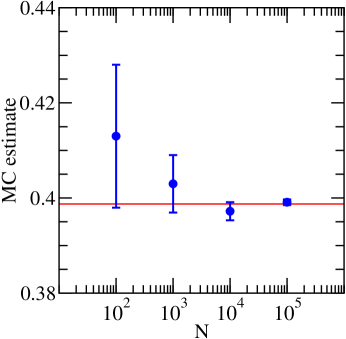
Figure 7: Monte Carlo estimates of the ratio of integrals $\int_{-\infty}^{\infty}g(x)h(x)dx\ /\int_{-\infty}^{\infty}h(x)dx$, where $g(x)=\cos(\sqrt{1+x^{2}})$ and $h(x)=e^{-x^{2}}/(x^{2}+2)$, against the number of Markov chain elements $N$ used. A simple Metropolis method was used with $h(x)$ as the sampling probability density. The horizontal line indicates the exact answer.

4 Monte Carlo study of the simple harmonic oscillator

As a first simple example, let us apply the Monte Carlo method to evaluate path integrals in the one-dimensional simple harmonic oscillator. The action in the imaginary time formalism is given by

$$S[x(\tau)]=\int_{\tau_{a}}^{\tau_{b}}\!d\tau\ \left(\textstyle\frac{1}{2}m\dot{x}^{2}+\frac{1}{2}m\omega^{2}x^{2}\right).$$

To carry out a Monte Carlo evaluation, it is necessary to discretize time $N\varepsilon=\tau_{b}-\tau_{a}$:

$$\frac{S}{\hbar}=\frac{m\varepsilon}{2\hbar}\!\sum_{j=0}^{N-1}\left[\left(\frac{x_{j+1}\!-\!x_{j}}{\varepsilon}\right)^{2}\!+\!\omega^{2}\left(\frac{x_{j+1}\!+\!x_{j}}{2}\right)^{2}\right],$$

where $\varepsilon$ should be chosen so discretization errors are sufficiently small. Introduce the dimensionless parameters

$$x_{k}=d_{k}\sqrt{\frac{\varepsilon\hbar}{m}},\qquad\kappa=\frac{1}{4}\varepsilon^{2}\omega^{2},$$

so that the action can be written

$$\frac{S}{\hbar}=\frac{1}{2}\!\sum_{j=0}^{N-1}\left[(d_{j+1}\!-\!d_{j})^{2}\!+\!\kappa(d_{j+1}\!+\!d_{j})^{2}\right],$$

and with a few more manipulations, the action becomes

$$\frac{S}{\hbar}=\frac{1}{2}(1+\kappa)(d_{0}^{2}+d_{N}^{2})+(1\!+\!\kappa)\!\left[\sum_{j=1}^{N-1}d_{j}^{2}\right]-(1\!-\!\kappa)\!\left[\sum_{j=0}^{N-1}d_{j}d_{j+1}\right].$$

The first constant is irrelevant, so it can be discarded, then one last rescaling

$$u_{j}=d_{j}\sqrt{1+\kappa},\quad g=\frac{1-\kappa}{1+\kappa},\quad d_{0}=d_{N}=0,$$

yields the final form for the action:

$$\frac{S}{\hbar}=\left[\sum_{j=1}^{N-1}u_{j}^{2}\right]-g\!\left[\sum_{j=0}^{N-1}u_{j}u_{j+1}\right].$$

In this form, we have set $u_{0}=u_{N}=0$, which is tantamount to requiring $x_{a}=x_{b}=0$. The observables we will compute will be independent of the choice of the initial $x_{a}$ and final $x_{b}$ locations of the particle. A given path is specified by a vector $\mathbf{u}$ whose $N-1$ components are $u_{j}$ for $j=1,2,\dots,N-1$.

We must now devise an auxiliary proposal density in order to produce a Markov chain using the Metropolis-Hastings method. There is considerable freedom in designing such a proposal. If we use an auxiliary proposal that simultaneously changes all $N-1$ components of $\mathbf{u}$, one finds that the resulting changes to the action are rather large, and the acceptance probability becomes nearly zero. In order to get a reasonable acceptance rate, we must make only small changes to the action. This can be accomplished most easily if we only change one of the $u_{j}$ at a time. The most natural way to proceed is to randomly pick one time slice and perform a local update of that time slice. If equal probabilities are assigned to each time slice, then detailed balance is maintained and covering the entire hypervolume of integration is ensured.

A simple procedure for updating the path $\mathbf{u}\rightarrow\mathbf{u}^{\rm new}$ is as follows:

1. Randomly choose an integer $j$ from 1 to $N_{t}-1$, where $N_{t}$ is the number of time slices, with equal probability.

2. Propose a random shift $u_{j}\rightarrow\tilde{u}_{j}=u_{j}+\delta$ with $\delta$ chosen with uniform probability density in the range $-\Delta\leq\delta\leq\Delta$.

3. Calculate the change $\delta S$ in the action:

   $$\delta S/\hbar=\delta\ \left(\delta+2u_{j}-g(u_{j-1}+u_{j+1})\right).$$

4. Since $R(\tilde{u}_{j}\leftarrow u_{j})=R(u_{j}\leftarrow\tilde{u}_{j})$, then accept the proposed value $u_{j}^{\rm new}=\tilde{u}_{j}$ with probability $\min(1,e^{-\delta S/\hbar})$. If not accepted, then retain the old value: $u_{j}^{\rm new}=u_{j}$.

5. Repeat the above procedure $N_{t}$ times to constitute one updating sweep.

The rule of thumb for setting the value of $\Delta$ is to achieve an acceptance rate around 50%. A lower rate means that too much time is being wasted with rejections, whereas a higher rate means that the Markov chain might be moving through the integration hypervolume too slowly.

To start the Markov chain, one can either choose a random path (hot start) or choose $u_{j}=0$ for all $j$ (cold start). One then updates $N_{\rm therm}$ number of sweeps until the fixed point of the chain is reached (thermalization); usually, a few simple observables are monitored. Once the Markov chain is thermalized, the “measurements” can begin. The parameters in the simulation are chosen according to the following guidelines:

• Choose $\varepsilon$ so that discretization errors are sufficiently small.

• Choose $\Delta$ for an adequate acceptance rate.

• Choose the number of sweeps $N_{\rm sweeps}$ between measurements to achieve sufficiently small autocorrelations.

• Choose the number of measurements $N_{\rm meas}$ to achieve the desired precision in the results.

The results of some actual Monte Carlo computations using $\omega\varepsilon=0.25$ with $N_{t}=1000$ time slices are shown in Figs. 8-10. The Metropolis acceptance rate is shown in the left-hand plot in Fig. 8. To get an acceptance rate around 0.5-0.6, one sees that $\Delta=1.5$ is a good choice for $\omega\varepsilon=0.25$. Autocorrelations were monitored using a typical observable chosen to be $\langle u(\tau_{0}+5)u(\tau_{0})\rangle$, where $\tau_{0}$ is taken near the midpoint between the path end-points (we actually averaged over a large number of $\tau_{0}$ values in the middle region for increased statistics). The autocorrelation function for this observable is shown in the right-hand plot of Fig. 8 (dashed line). One sees that about 100 sweeps are needed to reduce autocorrelations down to the level of 0.1.

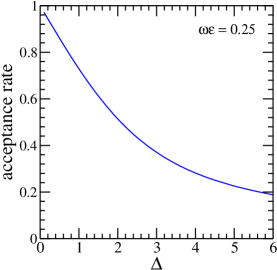
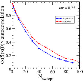
Figure 8: Left: Metropolis acceptance rate versus the parameter $\Delta$ for the simple harmonic oscillator with $\omega\varepsilon=0.25$. Right: Autocorrelation function associated with $\langle u(\tau_{0}+5)x(\tau_{0})\rangle$ against the number of Metropolis sweeps for updating the time slices $u_{j}$ sequentially (solid line) and randomly (dashed). When updating the time slices in random order, a sweep refers to $N_{t}$ successive local updates, where $N_{t}$ is the number of time slices.

Updating the path one $u_{j}$ at a time in random order with each $j$-value being equally likely to be chosen ensures detailed balance and coverage of the entire integration volume. But a simpler method would be to just sequentially sweep through the $u_{j}$, updating each $u_{j}$ one at a time. With much less calls to the random number generator, sequential sweeps would take less computer time. Coverage of the entire integration volume is again ensured, but detailed balance is lost. However, detailed balance was useful only in that it ensured that the ergodic Markov chain had a unique fixed-point. Even though detailed balance is lost when sequentially sweeping through the time slices, the fixed-point condition is maintained. Thus, sequential sweeps are totally acceptable. When updating randomly chosen $u_{j}$, the Markov matrix $\mathbf{P}$ is the same for each local update. When updating $u_{j}$ sequentially, the Markov matrix is different for each local update. However, the Markov matrix for an entire sweep $\mathbf{P}_{\rm sweep}$, being the product of the Markov matrices for each time slice, is the same for each sweep. So the theoretical foundations described previously still apply, as long as we apply them to $\mathbf{P}_{\rm sweep}$. The autocorrelation function for the observable $\langle u(\tau_{0}+5)u(\tau_{0})\rangle$ when updating time slices sequentially is shown as a solid line in the right-hand plot of Fig. 8. One sees that there is no adverse affect on the autocorrelations.

Portions of paths produced in an actual Markov chain with sequential time-slice updating for $\omega\varepsilon=0.25,N_{t}=1000,\Delta=1.5$ are shown in Fig. 9. Monte Carlo estimates for the correlation function $\langle u(\tau_{0}+\tau)u(\tau_{0})\rangle\rangle$ as a function of $\tau$ are compared to exact results in Fig. 10.

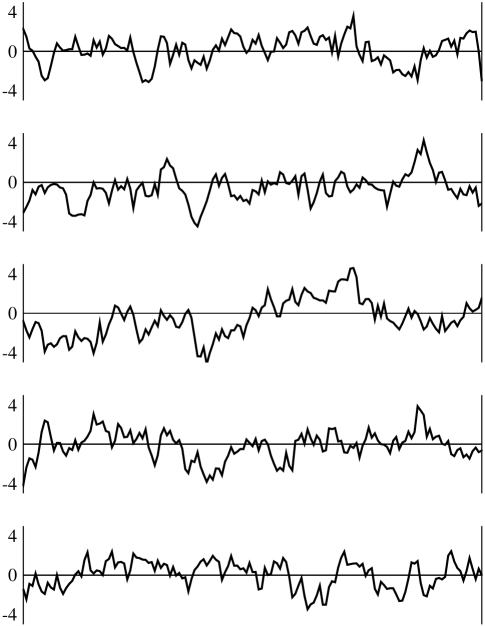
Figure 9: A few paths $u_{j}$ for $j=400-550$ with $N_{t}=1000$ from an actual Monte Carlo simulation of the simple harmonic oscillator with $\omega\varepsilon=0.25$.

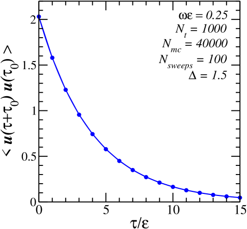
Figure 10: Monte Carlo estimates (circles) of the correlation function $\langle u(\tau_{0}+\tau)u(\tau_{0})\rangle$ are compared to the exact results (solid line) for the simple harmonic oscillator with $\omega\varepsilon=0.25$.

5 Monte Carlo calculations in real scalar field theory in 2+1 dimensions

The action for a real scalar field in continuous Euclidean $D$-dimensional space-time in the imaginary time formalism is given by

$$S=\int\!d^{D}x\ \left(\frac{1}{2}\partial_{\mu}\varphi(x)\partial_{\mu}\varphi(x)+\frac{1}{2}m^{2}\varphi(x)^{2}+\frac{g}{4!}\varphi(x)^{4}\right).$$

Note that the action must be dimensionless in natural units $\hbar=c=1$, and since $m$ has units of a derivative $\partial_{\mu}$, that is, of a mass, then the field must have dimension $[\varphi]=[m]^{\frac{1}{2}D-1}$, requiring that the coupling $g$ has units $[g]=[m]^{4-D}$. Thus, the coupling is dimensionless in 4 space-time dimensions, but has units of mass in 3 space-time dimensions, leaving $g/m$ dimensionless. We require $g\geq 0$ or the action will have no minimum.

Quantization of this field theory can be accomplished using path integrals, but the notion of a “path” must be generalized: a path here is a field configuration in both space and time. The path integral now consists of integrations over all field configurations. For a real scalar field, we now have an integral $-\infty\leq\varphi(x)\leq\infty$ at every space-time point $x$. The time-ordered two-point function is given by

$$\langle T\varphi(x_{1})\varphi(x_{2})\rangle=\frac{\int{\cal D}\varphi\ \varphi(x_{1})\varphi(x_{2})\exp(-S[\varphi])}{\int{\cal D}\varphi\ \exp(-S[\varphi])},$$

which generalizes to $n$-point functions, time-ordered product of $n$ fields, in a straightforward manner.

A Monte Carlo study requires an action on a space-time lattice. We will use an anisotropic cubic lattice with temporal lattice spacing $a_{t}$ and spatial lattice spacing $a_{s}$. Discretization of the action is achieved by replacing field derivatives by the simplest finite differences, and integrals over space-time by suitable summations over space-time lattice sites. The action is given by

$$S = a_{s}^{D-1}a_{t}\sum_{x}\!\left(\!\!\sum_{\mu}\frac{(\varphi(x\!+\!a_{\mu}\hat{\mu})\!-\!\varphi(x))^{2}}{2a_{\mu}^{2}}\!+\!\frac{1}{2}m^{2}\varphi(x)^{2}\!+\!\frac{g}{4!}\varphi(x)^{4}\right),$$

$$= a_{s}^{D-1}a_{t}\!\!\sum_{x}\!\!\left(\!\!-\!\!\sum_{\mu}\!\frac{\varphi(x\!+\!a_{\mu}\hat{\mu})\varphi(x)}{a_{\mu}^{2}}\!\!+\!\!\frac{1}{2}\!\left(\!\!m^{2}\!\!+\!\!\sum_{\nu}\!\frac{2}{a_{\nu}^{2}}\!\!\right)\!\!\varphi(x)^{2}\!\!+\!\!\frac{g}{4!}\varphi(x)^{4}\!\!\right),$$

where $a_{\mu}$ is the lattice spacing in the $\mu$ direction. Redefine the field $\sqrt{a_{s}^{D-3}a_{t}}\ \varphi(x)=\sqrt{2\kappa_{s}}\ \phi(x)$, where $\kappa_{s}$ is a dimensionless number, so the new field $\phi(x)$ is dimensionless. Then introduce a few more dimensionless parameters:

$$a_{s}/a_{t}=\zeta,\quad\lambda=\frac{g\zeta\kappa_{s}^{2}}{6a_{s}^{D-4}},$$

$$\kappa_{s}(a_{s}^{2}m^{2}+2\zeta^{2}+2D-2)=1-2\lambda,\quad\kappa=\zeta\kappa_{s},$$

to obtain the final form for the lattice action:

$$S = \sum_{x}\biggl{(}-\frac{2\kappa}{\zeta}\sum_{j=1}^{D-1}\phi(x)\phi(x\!+\!a_{s}\hat{j})-2\kappa\zeta\,\phi(x)\phi(x\!+\!a_{t}\hat{t})$$

$$\qquad\qquad+(1-2\lambda)\phi(x)^{2}+\lambda\phi(x)^{4}\biggr{)}.$$

The hopping parameter $\kappa$ essentially sets the mass parameter, and $\lambda\geq 0$ is the interaction strength. In what follows, we shall focus solely on the above theory in 3 space-time dimensions.

5.1 Exact results in free field limit $\lambda=0$

The free field theory $\lambda=0$ is exactly solvable. In this case, the path integrals are multivariate gaussians. The free action can be written in the form

$$S[\phi]={\textstyle\frac{1}{2}}\sum_{xy}\phi(x)M(x,y)\phi(y).$$

For $N$ lattice sites, $M$ is a real and symmetric $N\times N$ matrix having positive eigenvalues and given by

$$M(x,y) = -\frac{2\kappa}{\zeta}\sum_{j=1}^{D-1}\!\!\left(\delta(y,x\!+\!a_{s}\hat{j})+\delta(x,y\!+\!a_{s}\hat{j})\right)$$

$$-2\kappa\zeta\,\left(\delta(y,x\!+\!a_{t}\hat{t})+\delta(x,y\!+\!a_{t}\hat{t})\right)+2\delta(x,y).$$

The path integrals encountered in the free field theory can be evaluated using the so-called $J$-trick: use derivatives with respect to an external source $J_{k}$, followed by the limit $J_{k}\rightarrow 0$, to evaluate all integrals involving any number of products of the fields:

$$\prod_{i=1}^{N}\left(\int_{-\infty}^{\infty}\!\!d\phi_{i}\right)\phi_{m_{1}}\phi_{m_{2}}\dots\phi_{m_{r}}\ \exp(-{\textstyle\frac{1}{2}}\phi_{j}M_{jk}\phi_{k})$$

$$= \lim_{J_{n}\rightarrow 0}\frac{\delta}{\delta J_{m_{1}}}\cdots\frac{\delta}{\delta J_{m_{r}}}\prod_{i=1}^{N}\left(\int_{-\infty}^{\infty}\!\!d\phi_{i}\right)\ \exp(-{\textstyle\frac{1}{2}}\phi_{j}M_{jk}\phi_{k}+J_{n}\phi_{n}),$$

$$= \lim_{J_{n}\rightarrow 0}\frac{\delta}{\delta J_{m_{1}}}\cdots\frac{\delta}{\delta J_{m_{r}}}\left(\det\left(\frac{M}{2\pi}\right)\right)^{-1/2}\!\!\exp\left(\textstyle\frac{1}{2}J_{j}M^{-1}_{jk}J_{k}\right).$$

This trick does the Wick contractions automagically!

The two-point function is given by $\langle T\phi(x_{1})\phi(x_{2})\rangle=M^{-1}(x_{1},x_{2})$. The inverse of $M$ can be obtained by the method of Green functions and using Fourier transforms. For an $L_{x}\times L_{y}\times L_{t}$ lattice, the result is

$$M^{-1}(x,y)=\frac{\zeta}{2\kappa L_{x}L_{y}L_{t}}\sum_{k_{\mu}}\frac{\cos(k\!\cdot\!(x\!-\!y))}{(a_{s}^{2}m^{2}+4\sum_{j=1}^{2}\sin^{2}({\textstyle\frac{1}{2}}k_{j})+4\zeta^{2}\,\sin^{2}({\textstyle\frac{1}{2}}k_{t}))},$$

where $k_{\mu}=2\pi n_{\mu}/L_{\mu}$ for $n_{\mu}=0,1,2,\dots,L_{\mu}-1$. The pole in the two-point function gives the energy $a_{t}E_{p}$ of a single particle of momentum $a_{s}p$:

$$a_{t}E_{p}=2\sinh^{-1}\left(\frac{1}{2\zeta}\sqrt{a_{s}^{2}m^{2}+4\sin^{2}({\textstyle\frac{1}{2}}a_{s}p_{x})+4\sin^{2}({\textstyle\frac{1}{2}}a_{s}p_{y})}\right).$$

For small $a_{t},a_{s}$, this becomes $E_{p}=\sqrt{m^{2}+p_{x}^{2}+p_{y}^{2}}$. The spectrum is the sum of free particle energies.

5.2 Metropolis updating

The Metropolis-Hastings method is useful only when the auxiliary proposal density leads to a reasonable acceptance rate, typically around 0.5. If we simultaneously change field values at all lattice sites, the value of the action most likely changes by a large amount, and the Metropolis-Hastings acceptance probability plummets to zero. However, if we propose a change only to the field value on one site, a reasonable acceptance rate can be achieved. To maintain detailed balance and ensure coverage of the entire integration region, the site to be updated should be chosen randomly, with each site being equally likely to be selected. However, as in the case of the simple harmonic oscillator, one finds that updating the fields at sites selected sequentially, sweeping through the lattice, works just as well. Although detailed balance is lost, the crucial fixed-point condition is maintained, and by sequentially visiting every site, coverage of the entire integration region is ensured.

Thus, we shall use an auxiliary proposal probability density that sweeps through the lattice, visiting each lattice site sequentially, updating each and every site one at a time. In the battle against autocorrelations, we expect that such a local updating scheme should be effective in treating the small wavelength modes of the theory, but the long wavelength modes may not be dealt with so well.

Recall that the action is

$$S = \sum_{x}\biggl{(}-\frac{2\kappa}{\zeta}\sum_{j=1}^{D-1}\phi(x)\phi(x\!+\!a_{s}\hat{j})-2\kappa\zeta\,\phi(x)\phi(x\!+\!a_{t}\hat{t})$$

$$\qquad\qquad+(1-2\lambda)\phi(x)^{2}+\lambda\phi(x)^{4}\biggr{)}.$$

Define the neighborhood $N(x)$ of the site $x$ by

$$N(x)=-\frac{2\kappa}{\zeta}\sum_{j=1}^{D-1}\Bigl{(}\phi(x+a_{s}\hat{j})+\phi(x-a_{s}\hat{j})\Bigr{)}-2\kappa\zeta\,\Bigl{(}\phi(x+a_{t}\hat{t})+\phi(x-a_{t}\hat{t})\Bigr{)}.$$

If the field at the one site $x$ is changed $\phi(x)\rightarrow\phi(x)+\Delta$, then the change in the action is

$$\delta S=\Delta\biggl{(}N(x)+(\Delta+2\phi(x))\biggl{(}1+\lambda\Bigl{(}(\Delta+2\phi(x))\Delta+2(\phi(x)^{2}-1)\Bigr{)}\biggr{)}\biggr{)}.$$

This change in the action can also be written

$$\delta S = \Delta\,(a_{0}+a_{1}\Delta+a_{2}\Delta^{2}+a_{3}\Delta^{3}),$$

$$a_{0} = N(x)+2\phi(x)(1+2\lambda(\phi(x)^{2}-1)),$$

$$a_{1} = 1+2\lambda(3\phi(x)^{2}-1),$$

$$a_{2} = 4\lambda\phi(x),$$

$$a_{3} = \lambda.$$

Single-site updates involve a single continuous real variable $\phi$. A simple proposal density is then

$$R(\widetilde{\phi}\leftarrow\phi)=\left\{\begin{array}[]{l@{\hspace{1cm}}l}\displaystyle\frac{1}{2\Delta_{0}},\hfil\hskip 28.45274pt&-\Delta_{0}\leq(\widetilde{\phi}-\phi)\leq\Delta_{0},\\[10.0pt] 0,\hfil\hskip 28.45274pt&|\widetilde{\phi}-\phi|>\Delta_{0}.\end{array}\right.$$

In other words, a value for $\Delta$ is chosen randomly with uniform probability density in the range $-\Delta_{0}\leq\Delta\leq\Delta_{0}$, and the proposed value for the field is $\phi(x)+\Delta$. The width $\Delta_{0}$ is chosen to obtain an acceptance rate around 50%. The proposed new value is accepted with probability $\min(1,\exp(-\delta S))$. If rejected, the current field value is retained. This single-site procedure is repeated at every site on the lattice, sequentially sweeping through the lattice.

5.3 Microcanonical updating

When the single particle mass $a_{t}m_{\rm gap}$ is small, the coherence length $\xi=1/(a_{t}m_{\rm gap})$ becomes large. The so-called continuum limit of the theory is reached when the coherence length is large compared to the lattice spacing, that is, when $\xi\rightarrow\infty$. However, $\xi\rightarrow\infty$ only occurs near a second order phase transition (a critical point). One finds that autocorrelations with the above Metropolis updating scheme become long ranged as $\xi$ becomes large; this is known as critical slowing down. Autocorrelations are problematic even for $\xi\approx 5$ with the above Metropolis updating. In such cases, we will need to use some other procedure to better update the long wavelength modes.

Long wavelength modes are associated with lower frequencies and lower energies. In other words, long-wavelength modes are associated with very small changes to the action. A possible way to improve autocorrelations is to make large but action preserving $\delta S=0$ changes to the field at one site. We shall refer to this as a microcanonical update, but such schemes are often referred to as overrelaxation in the literature. Local updating is so easy, we do not want to give up on it yet! In devising our microcanonical updating scheme, we must ensure that the fixed-point of our Markov chain is unaffected. Note that microcanonical updating cannot be used just by itself since it does not explore the entire integration region. Microcanonical updating must be used in combination with some scheme that does cover the entire integration volume, such as the above-described Metropolis sweeps.

To facilitate the discussion of such microcanonical updating, let us first revisit the Metropolis-Hastings method, examining the case of a sharply-peaked proposal probability density. Suppose $f(\phi)$ is a well-behaved, single-valued, invertible function, then consider a proposal density given by a Breit-Wigner peaked about $f(\phi)$:

$$R_{f}(\widetilde{\phi}\leftarrow\phi)=\frac{1}{\pi}\frac{\varepsilon}{\Bigl{(}\widetilde{\phi}-f(\phi)\Bigr{)}^{2}+\varepsilon^{2}},$$

where $\varepsilon$ is a constant. Notice that this probability density is properly normalized:

$$\int_{-\infty}^{\infty}\!d\widetilde{\phi}\ R_{f}(\widetilde{\phi}\leftarrow\phi)=1.$$

With such a proposal density, the standard choice for the acceptance probability which satisfies detailed balance is given, as usual, by

$$P_{\rm acc}(\widetilde{\phi}\!\leftarrow\!\phi)\!=\!\min\!\!\left(\!\!1,\!\frac{R_{f}(\phi\!\leftarrow\!\widetilde{\phi})\pi(\widetilde{\phi})}{R_{f}(\widetilde{\phi}\!\leftarrow\!\phi)\pi(\phi)}\!\!\right)\!\!=\!\min\!\!\left(\!\!1,\!\frac{\Bigl{(}\!(\widetilde{\phi}\!-\!f(\phi))^{2}\!+\!\varepsilon^{2}\!\Bigr{)}\pi(\widetilde{\phi})}{\Bigl{(}\!(\phi\!-\!f(\widetilde{\phi}))^{2}\!+\!\varepsilon^{2}\!\Bigr{)}\pi(\phi)}\!\!\right).$$

As $\varepsilon$ becomes very small, the proposal density becomes very sharply peaked about $\widetilde{\phi}=f(\phi)$. In fact, we are interested in taking the limit $\varepsilon\rightarrow 0$ to obtain a Dirac $\delta$-function:

$$\delta(x)=\frac{1}{\pi}\lim_{\varepsilon\rightarrow 0}\frac{\varepsilon}{x^{2}+\varepsilon^{2}}.$$

The probability of proposing a $\widetilde{\phi}$ value between $f(\phi)-\varepsilon\leq\widetilde{\phi}\leq f(\phi)+\varepsilon$ is given by

$$\int_{f(\phi)-\varepsilon}^{f(\phi)+\varepsilon}\!\!d\widetilde{\phi}\ R_{f}(\widetilde{\phi}\leftarrow\phi)=\frac{1}{2}.$$

However, we need to consider a range of values which tends to a single value but for which the probability tends to unity as $\varepsilon\rightarrow 0$. Clearly, a larger range is needed. The probability of proposing a value between $f(\phi)-\sqrt{\varepsilon}\leq\widetilde{\phi}\leq f(\phi)+\sqrt{\varepsilon}$ is

$$\int_{f(\phi)-\sqrt{\varepsilon}}^{f(\phi)+\sqrt{\varepsilon}}\!\!d\widetilde{\phi}\ R_{f}(\widetilde{\phi}\leftarrow\phi)=\frac{2}{\pi}\tan^{-1}\left(\frac{1}{\sqrt{\varepsilon}}\right),$$

which does tends to unity as $\varepsilon\rightarrow 0$. If $f(\phi)$ is more than $\sqrt{\varepsilon}$ away from $\phi$, then the probability that the transition is actually made is

$$\int_{f(\phi)-\sqrt{\varepsilon}}^{f(\phi)+\sqrt{\varepsilon}}\!\!d\widetilde{\phi}\ W_{f}(\widetilde{\phi}\leftarrow\phi)=\int_{f(\phi)-\sqrt{\varepsilon}}^{f(\phi)+\sqrt{\varepsilon}}\!\!d\widetilde{\phi}\ P_{\rm acc}(\widetilde{\phi}\leftarrow\phi)R_{f}(\widetilde{\phi}\leftarrow\phi).$$

Given that $R_{f}(\widetilde{\phi}\leftarrow\phi)$ is always positive, the above integral is given by

$$\min\left(\frac{2}{\pi}\tan^{-1}\left(\frac{1}{\sqrt{\varepsilon}}\right),\ \frac{1}{\pi}\int_{f(\phi)-\sqrt{\varepsilon}}^{f(\phi)+\sqrt{\varepsilon}}\!\!d\widetilde{\phi}\frac{\varepsilon\ \pi(\widetilde{\phi})}{\Bigl{(}(\phi-f(\widetilde{\phi}))^{2}+\varepsilon^{2}\Bigr{)}\pi(\phi)}\right).$$

If we write $\widetilde{\phi}=f(\phi)+y$, then the remaining integral above becomes

$$\frac{1}{\pi}\int_{-\sqrt{\varepsilon}}^{\sqrt{\varepsilon}}\!\!dy\frac{\varepsilon\ \pi(f(\phi)+y)}{\Bigl{(}(\phi-f(f(\phi)+y))^{2}+\varepsilon^{2}\Bigr{)}\pi(\phi)}.$$

Now consider two cases: (a) $f(f(\phi))\neq\phi$, and (b) $f(f(\phi))=\phi$.

For the first case when $f(f(\phi))\neq\phi$, since we are integrating over such a small range, the series expansion of the integrand about the central $y=0$ point should approximate the true integrand well, assuming no singularities. Performing this expansion about $y=0$, then integrating, one finds a zero probability as $\varepsilon\rightarrow 0$, as long as $\pi(f(\phi))/\pi(\phi)$ is finite. To see this, begin by noting that the integral has the form

$$\frac{\varepsilon}{\pi}\int_{-\sqrt{\varepsilon}}^{\sqrt{\varepsilon}}\!\!dy\frac{(a_{0}+a_{1}y+a_{2}y^{2}+\dots)}{(\varepsilon^{2}+b_{0}+b_{1}y+b_{2}y^{2}+b_{3}y^{3}+\dots)},$$

where the $a_{j},b_{j}$ are constants. If the denominator does not become zero anywhere in the integration range, then the integral can be well approximated by

$$\frac{\varepsilon a_{0}}{\pi(b_{0}+\varepsilon^{2})}\int_{-\sqrt{\varepsilon}}^{\sqrt{\varepsilon}}\!\!dy\Bigl{(}1+c_{1}(\varepsilon)y+c_{2}(\varepsilon)y^{2}+c_{3}(\varepsilon)y^{3}+c_{4}(\varepsilon)y^{4}+\dots\Bigr{)}$$

$$=\frac{2\varepsilon^{3/2}a_{0}}{\pi(b_{0}+\varepsilon^{2})}\Bigl{(}1+\textstyle\frac{1}{3}\varepsilon c_{2}(\varepsilon)+\frac{1}{5}\varepsilon^{2}c_{4}(\varepsilon)+\cdots\Bigr{)}\rightarrow 0\ \mbox{as}\ \varepsilon\rightarrow 0\ \mbox{if}\ b_{0}\neq 0,$$

where the $c_{j}(\varepsilon)$ tend to finite constants as $\varepsilon\rightarrow 0$.

For the second case when $f(f(\phi))=\phi$, more care is needed when expanding about $y=0$ since the integral has the form

$$\frac{\varepsilon}{\pi}\int_{-\sqrt{\varepsilon}}^{\sqrt{\varepsilon}}\!\!dy\frac{(a_{0}+a_{1}y+a_{2}y^{2}+\dots)}{(\varepsilon^{2}+b_{2}y^{2}+b_{3}y^{3}+b_{4}y^{4}\dots)}.$$

To reproduce the integrand to a good approximation over the entire integration range, the $b_{2}y^{2}$ term must be retained in the denominator, and the rest of the function can be expanded about $y=0$:

$$\frac{\varepsilon}{\pi}\int_{-\sqrt{\varepsilon}}^{\sqrt{\varepsilon}}\!\!dy\frac{a_{0}}{(\varepsilon^{2}+b_{2}y^{2})}\left\{1+\frac{a_{1}}{a_{0}}y+\frac{a_{2}}{a_{0}}y^{2}+\left(\frac{a_{3}}{a_{0}}-\frac{b_{3}}{\varepsilon^{2}}\right)y^{3}+\dots\right\}.$$

For $b_{2}>0$, then the result of the integration is

$$\frac{2a_{0}}{\pi\sqrt{b_{2}}}\tan^{-1}\left(\sqrt{\frac{b_{2}}{\varepsilon}}\right)\left\{1+d_{1}\sqrt{\varepsilon}+d_{2}\varepsilon+d_{3}\varepsilon^{3/2}+\cdots\right\}.$$

Hence, the acceptance probability is given in the limit $\varepsilon\rightarrow 0$ by

$$P_{\rm acc}=\min\left(1,\frac{a_{0}}{\sqrt{b_{2}}}\right).$$

In this case, $a_{0}=\pi(f(\phi))/\pi(\phi)$ and $b_{2}=(f^{\prime}(f(\phi)))^{2}$, where the ^′ indicates the derivative function. If we differentiate both sides of $f(f(\phi))=\phi$ with respect to $\phi$, we see that for a self-inverse function,

$$1=\frac{d}{d\phi}\biggl{(}f(f(\phi))\biggr{)}=f^{\prime}(f(\phi))\ f^{\prime}(\phi),$$ (7)

so that for a self-inverse function,

$$\frac{1}{(f^{\prime}(f(\phi)))^{2}}=\left|\frac{f^{\prime}(\phi)}{f^{\prime}(f(\phi))}\right|\qquad\mbox{(self-inverse function)}.$$ (8)

Taking the limit $\varepsilon\rightarrow 0$, we have a proposal density and an acceptance probability given by

$$R_{f}(\widetilde{\phi}\leftarrow\phi) = \delta\Bigl{(}\widetilde{\phi}-f(\phi)\Bigr{)},\qquad f(f(\phi))=\phi,$$ (9)

$$P_{\rm acc}(\widetilde{\phi}\leftarrow\phi) = \min\left(1,\frac{\sqrt{|f^{\prime}(\phi)|}\ \pi(\widetilde{\phi})}{\sqrt{|f^{\prime}(\widetilde{\phi})|}\ \pi(\phi)}\right).$$ (10)

Now specialize to the case of microcanonical updating in which the self-inverse function $f(\phi)$ reflects the field in some way so as to preserve the action. Let $S(\phi)$ denote that part of the action which involves the field at the site $x$ being updated. If $\phi$ is the current value of the field at site $x$, then let $f(\phi)$ denote another value of the field for which $S(\phi)=S(f(\phi))$ so that $\pi(f(\phi))=\pi(\phi)$. For an infinitesimal change $\phi\rightarrow\phi+\delta\phi$, we have

$$S(\phi+\delta\phi)=S(f(\phi+\delta\phi)).$$

Expanding both sides,

$$S(\phi)+S^{\prime}(\phi)\delta\phi+O(\delta\phi^{2}) = S(f(\phi)+f^{\prime}(\phi)\delta\phi+O(\delta\phi^{2}))$$

$$= S(f(\phi))+S^{\prime}(f(\phi))\ f^{\prime}(\phi)\delta\phi+O(\delta\phi^{2})$$

$$= S(\phi)+S^{\prime}(f(\phi))\ f^{\prime}(\phi)\delta\phi+O(\delta\phi^{2}).$$

Solving this equation order by order in $\delta\phi$ leads to

$$S^{\prime}(\phi)=S^{\prime}(f(\phi))\ f^{\prime}(\phi)\quad\rightarrow\quad f^{\prime}(\phi)=\frac{S^{\prime}(\phi)}{S^{\prime}(f(\phi))}.$$

Hence,

$$f^{\prime}(f(\phi))=\frac{S^{\prime}(f(\phi))}{S^{\prime}(f(f(\phi)))}=\frac{S^{\prime}(f(\phi))}{S^{\prime}(\phi)}.$$

So the proposal and acceptance probability densities are

$$R_{f}(\widetilde{\phi}\leftarrow\phi) = \delta\Bigl{(}\widetilde{\phi}-f(\phi)\Bigr{)},\qquad f(f(\phi))=\phi,\quad S(f(\phi))=S(\phi),$$

$$P_{\rm acc}(\widetilde{\phi}\leftarrow\phi) = \min\left(1,\left|\frac{S^{\prime}(\phi)}{S^{\prime}(\widetilde{\phi})}\right|\right),\qquad\pi(\phi)=\frac{\exp(-S[\phi])}{\displaystyle\int{\cal D}\widetilde{\phi}\ \exp(-S[\widetilde{\phi}])}.$$

So far, we have examined only the case of applying a single self-inverse function which leaves the action invariant. In the $\phi^{4}$ field theory, the action preserving equation $\delta S=0$ will often have four solutions. In other words, more than one self-inverse action-preserving function are possible. The simplest way to proceed is to randomly pick one of the self-inverse action-preserving functions $f_{j}(\phi)$ with equal probabilities, then apply the accept-reject condition on the resulting field value $f_{j}(\phi)$.

The above procedure always proposes a change to the field, then an accept-reject step is applied. A straightforward modification of the above procedure is to not always propose a change. The above method can be generalized to include a probability $\mu$ of proposing a change; we will find that sometimes we will need $\mu<1$ to prevent (damped) oscillations in the autocorrelation function.

The summary of our microcanonical updating process is as follows:

1. Decide to propose a new field value with probability $\mu$. If the random decision is to retain the current field value, the steps below can be skipped.

2. Given initial value $\phi$ of the field at site $x$, solve $\delta S(\phi)=0$. Let $\phi_{j}$ denote the real solutions which differ from $\phi$. These will be the roots of a cubic polynomial. Sometimes there will be three such real distinct solutions, other times there will be only one. (The case of degenerate solutions is highly unlikely.)

3. With equal probability, randomly choose one of the $\phi_{j}$ as the proposed new field value. Let $\widetilde{\phi}$ denote the chosen value.

4. Accept this value with probability

   $$P_{\rm acc}(\widetilde{\phi}\leftarrow\phi)=\min\left(1,\left|\frac{S^{\prime}(\phi)}{S^{\prime}(\widetilde{\phi})}\right|\right).$$

   If rejected, the original value $\phi$ is retained.

The above procedure is repeated for each site, sequentially sweeping through the lattice. All of the above formulas have assumed that $S^{\prime}(\phi)\neq 0$ and $S^{\prime}(\phi_{j})\neq 0$. In the extremely unlikely case that any such minima, maxima, or inflection points are encountered, simply retain the original field value and move on to the next site.

5.4 Autocorrelations in the free field $\lambda=0$ theory

Let us first study autocorrelations in the free field $\lambda=0$ theory. The autocorrelation function $\rho(\tau)$ for the observable $\langle\Phi(t)\Phi(0)\rangle$ with $t=1/(2a_{s}m)$ and $\Phi(t)=\sum_{xy}\phi(x,y,t)$ is shown in Figs. 11-14 for various different updating schemes. The parameter $\tau$ is the number of compound sweeps, and $a_{s}m=0.10,0.25,0.50$ are used for $\lambda=0$ on $24^{3}$ isotropic lattices.

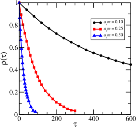
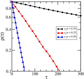
Figure 11: The autocorrelation function $\rho(\tau)$ for $\langle\Phi(t)\Phi(0)\rangle$ with $t=1/(2a_{s}m)$ and $\Phi(t)=\sum_{xy}\phi(x,y,t)$ using $a_{s}m=0.10,0.25,0.50$ and $\lambda=0$ on $24^{3}$ isotropic lattices. The parameter $\tau$ refers to the number of Metropolis sweeps. The right plot has a logarithmic vertical scale.

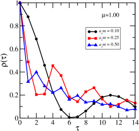
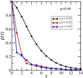
Figure 12: The autocorrelation function $\rho(\tau)$ for $\langle\Phi(t)\Phi(0)\rangle$ with $t=1/(2a_{s}m)$ and $\Phi(t)=\sum_{xy}\phi(x,y,t)$ using $a_{s}m=0.10,0.25,0.50$ and $\lambda=0$ on $24^{3}$ isotropic lattices. The parameter $\tau$ refers to the number of compound sweeps. Each compound sweep is one Metropolis sweep, followed by one microcanonical sweep with probability $\mu$ of proposing a change. In the left plot, $\mu=1$, whereas $\mu=0.98$ in the right plot.

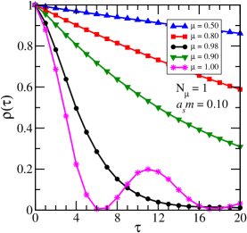
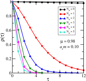
Figure 13: The autocorrelation function $\rho(\tau)$ for $\langle\Phi(t)\Phi(0)\rangle$ with $t=1/(2a_{s}m)$ and $\Phi(t)=\sum_{xy}\phi(x,y,t)$ using $a_{s}m=0.10$ only and $\lambda=0$ on $24^{3}$ isotropic lattices. The parameter $\tau$ refers to the number of compound sweeps. Each compound sweep is one Metropolis sweep, followed by $N_{\mu}$ microcanonical sweeps with probability $\mu$ of proposing a change. In the left plot, $N_{\mu}=1$ and $\mu$ is varied; in the right plot, $\mu=0.98$ and $N_{\mu}$ is varied.

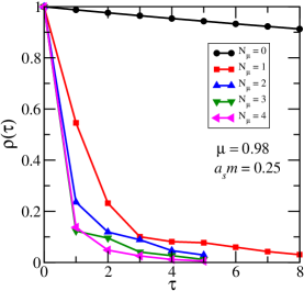
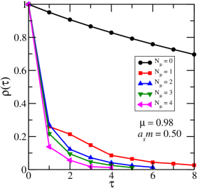
Figure 14: The autocorrelation function $\rho(\tau)$ for $\langle\Phi(t)\Phi(0)\rangle$ with $t=1/(2a_{s}m)$ and $\Phi(t)=\sum_{xy}\phi(x,y,t)$ using $a_{s}m=0.25$ (left plot) and $a_{s}m=0.50$ (right plot) and $\lambda=0$ on $24^{3}$ isotropic lattices. The parameter $\tau$ refers to the number of compound sweeps. Each compound sweep is one Metropolis sweep, followed by $N_{\mu}$ microcanonical sweeps with probability $\mu=0.98$ of proposing a change.

In Fig. 11, each compound sweep is just one Metropolis sweep. One sees that nearly 2200 sweeps are needed to reduce autocorrelations down to 0.1 for $a_{s}m=0.10$. Fig. 12 shows the dramatic reduction in autocorrelations by including microcanonical sweeps in the updating. Each compound sweep in this figure is one Metropolis sweep, followed by one microcanonical sweep with probability $\mu$ of proposing a change. The autocorrelation function has undesirable oscillations when $\mu=1$ in the free field theory, as shown in the left hand plot in this figure. These oscillations can be removed by using $\mu=0.98$, as shown in the right-hand plot of this figure.

In Figs. 13 and 14, each compound sweep is one Metropolis, followed by $N_{\mu}$ microcanonical sweeps with probability $\mu$ of proposing a change. In the left-hand plot of Fig. 13, $N_{\mu}=1$ is used and $\mu$ is varied. One sees that in the free scalar field theory, autocorrelations improve as $\mu$ increases towards unity, but $\mu=1$ introduces undesirable oscillations. Setting $\mu=0.98$ seems to be ideal. This value is used in the right-hand plot in this figure, and $N_{\mu}$ is varied. This plot shows autocorrelations improving as $N_{\mu}$ increases, but there are diminishing returns. As $N_{\mu}$ increases, each compound sweep takes significantly more time, so this has to be weighed against the improvement in the autocorrelations. One finds that $N_{\mu}=3$ seems optimal in the case of $a_{s}m=0.10$. The autocorrelations for different $N_{\mu}$ with $\mu=0.98$ fixed are also shown in Fig. 14 for $a_{s}m=0.25$ (left plot) and $a_{s}m=0.50$ (right plot). There is a dramatic improvement in going from $N_{\mu}=0$ to $N_{\mu}=1$, but there is no further gain in increasing $N_{\mu}$ any further for these mass parameters.

5.5 Extracting observables

The stationary-state energies can be extracted from the asymptotic decay rates of temporal correlations of the fields. The temporal evolution of the field as a Heisenberg-picture quantum operator is

$$\phi(t)=e^{Ht}\phi(0)e^{-Ht},$$

and under certain general assumptions (an action satisfying both link and site reflection positivity) and ignoring temporal boundary conditions, then for $t\geq 0$,

$$\langle 0|\phi(t)\phi(0)|0\rangle = \sum_{n}\langle 0|e^{Ht}\phi(0)e^{-Ht}|n\rangle\langle n|\phi(0)|0\rangle,$$

$$= \sum_{n}\Bigl{|}\langle n|\phi(0)|0\rangle\Bigr{|}^{2}e^{-(E_{n}-E_{0})t}=\sum_{n}A_{n}e^{-(E_{n}-E_{0})t},$$

where a complete set of (discrete) eigenstates of $H$ satisfying $H|n\rangle=E_{n}|n\rangle$ has been inserted. Note that on a lattice with periodic boundary conditions, momentum is discrete, so the energy eigenstates are also discrete. If $\langle 1|\phi(0)|0\rangle\neq 0$, then $A_{1}$ and $E_{1}-E_{0}$ can be extracted as $t$ becomes large, assuming $\langle 0|\phi(0)|0\rangle=0$. One can use any operator $O(t)$ which is a function of the field $\phi(t)$ only on a time slice $t$. The extraction of $A_{1}$ and $E_{1}-E_{0}$ is done using a correlated$-\chi^{2}$ fit:

$$\chi^{2}=\sum_{tt^{\prime}}\Bigl{(}C(t)-M(t,\alpha)\Bigr{)}\sigma_{tt^{\prime}}^{-1}\Bigl{(}C(t^{\prime})-M(t^{\prime},\alpha)\Bigr{)},$$

where $C(t)$ represents the Monte Carlo estimates of the correlation function with covariance matrix $\sigma_{tt^{\prime}}$ and the model function is $M(t,\alpha)=\alpha_{1}e^{-\alpha_{0}t}$. The covariance matrix $\sigma_{tt^{\prime}}$ is determined using the standard Monte Carlo variance formula. To determine estimates of the model parameters $\alpha_{0}$ and $\alpha_{1}$, one minimizes the above $\chi^{2}$ with respect to the model parameters. Uncertainties in the best-fit parameters $\alpha_{0}=E_{1}-E_{0}$ and $\alpha_{1}=A_{1}$ are usually obtained by a jackknife or bootstrap procedure (more on this in a moment). The fit must be done for a time range $t_{\rm min}\leq t\leq t_{\rm max}$ such that an acceptable fit quality is obtained, that is, $\chi^{2}/\mbox{dof}\approx 1$. A sum of two-exponentials as a model function can be used to minimize sensitivity to $t_{\rm min}$, but the fit parameters associated with faster-decaying exponential are generally not good estimates of the gap to the next energy level and should be discarded.

The Monte Carlo method exploits the central limit theorem to determine the statistical uncertainty in the covariance matrix $\sigma_{tt^{\prime}}$. But how can one determine the uncertainty in the fit parameters $\alpha_{0}$ and $\alpha_{1}$? These are not simple quantities that can be defined properly on a single path; the Monte Carlo variance formula cannot be easily applied. The use of resampling schemes solves this problem. Let $\langle f\rangle$ denote the Monte Carlo estimate of some quantity $f$ using all $X_{k}$ elements in a Markov chain, for $k=1,2,\dots,N$, and let $\langle f\rangle_{J}$ denote the Monte Carlo estimate of $f$ omitting $X_{J}$ (so only the other $N-1$ $X_{k}$ values are used). The so-called jackknife error estimate in $\langle f\rangle$ is given by

$$\sigma^{(J)} = \left(\frac{N-1}{N}\sum_{J=1}^{N}(\langle f\rangle_{J}-\langle f\rangle)^{2}\right)^{1/2},$$

$$\langle f\rangle = \frac{1}{N}\sum_{k=1}^{N}f(X_{k}),\qquad\langle f\rangle_{J}=\frac{1}{N-1}\sum_{k\neq J}f(X_{k}).$$

Again, the Monte Carlo variance formula can be used to determine the covariance matrix $\sigma_{tt^{\prime}}$ for the correlation function itself in $\chi^{2}$, and the jackknife method gives an estimate of the errors in the model fit parameters.

Another resampling scheme is the bootstrap. Again, let $\langle f\rangle$ denote the Monte Carlo estimate of some quantity $f$ using all $X_{k}$ for $k=1,2,\dots,N$, and let $\langle f\rangle_{b}$ denote the Monte Carlo estimate of $f$ using a new set $\widehat{X}_{k}$, for $k=1,2,\dots,N$, where each $\widehat{X}_{k}$ is one of the original $X_{j}$ chosen randomly with equal probability (a bootstrap sample). A given $X_{j}$ can occur multiple times in the bootstrap sample. After one obtains a large number $B$ of such estimates, then the following quantity $\widehat{\langle f\rangle}=(1/B)\sum_{b=1}\langle f\rangle_{b}$ is evaluated. The bootstrap error is given by

$$\sigma^{(B)}=\left(\frac{1}{B-1}\sum_{b=1}^{B}(\langle f\rangle_{b}-\widehat{\langle f\rangle})^{2}\right)^{1/2}.$$

For a given quantity, a plot of its probability distribution can be obtained from its $B$ bootstrap estimates.

A particularly good visual tool to see how well an energy can be extracted is the so-called effective mass. For a correlator $C(t)$, the effective mass is defined by

$$m_{\rm eff}(t)=\ln\left(\frac{C(t)}{C(t+a_{t})}\right).$$

This is a function which tends to $E_{1}-E_{0}$ as $t$ becomes large:

$$m_{\rm eff}(t) = \ln\left(\frac{A_{1}e^{-(E_{1}-E_{0})t}\Bigl{(}1+(A_{2}/A_{1})e^{-(E_{2}-E_{1})t}+\dots\Bigr{)}}{A_{1}e^{-(E_{1}-E_{0})(t+a_{t})}\Bigl{(}1\!+\!(A_{2}/A_{1})e^{-(E_{2}-E_{1})(t+a_{t})}\!+\!\dots\!\!\!\Bigr{)}}\right),$$

$$= \ln\left(\frac{e^{(E_{1}-E_{0})a_{t}}\Bigl{(}1+(A_{2}/A_{1})e^{-(E_{2}-E_{1})t}+\dots\Bigr{)}}{\Bigl{(}1\!+\!(A_{2}/A_{1})e^{-(E_{2}-E_{1})(t+a_{t})}\!+\!\dots\!\!\!\Bigr{)}}\right),$$

$$\stackrel{{\scriptstyle t\rightarrow\infty}}{{\longrightarrow}} \ln\left(e^{(E_{1}-E_{0})a_{t}}\right)=a_{t}(E_{1}-E_{0}).$$

The value $E_{1}-E_{0}$ is seen as a large-time plateau in the effective mass. Contributions from faster-decaying exponentials are seen as deviations of the effective mass from its asymptotic plateau value. A “good” operator with little coupling to higher-lying states results in a rapid onset of the plateau. Statistical noise generally grows with $t$.

Extracting more than just the lowest energy in a symmetry channel requires a hermitian matrix of correlation functions $C_{ij}(t)$. Let $\lambda_{n}(t,t_{0})$ denote the eigenvalues of $C(t_{0})^{-1/2}\,C(t)\,C(t_{0})^{-1/2}$, where $t_{0}$ is some fixed reference time. These eigenvalues can be viewed as principal correlators. Assume that they are ordered such that $\lambda_{0}\geq\lambda_{1}\geq\cdots$ as $t$ becomes large, then one can show that

$$\lim_{t\rightarrow\infty}\lambda_{n}(t,t_{0}) = e^{-E_{n}(t-t_{0})}\Bigl{(}1+O(e^{-\Delta_{n}(t-t_{0})})\Bigr{)},$$

$$\Delta_{n} = \min_{k\neq n}|E_{k}-E_{n}|.$$

The effective masses associated with these principal correlators are known as principal effective masses:

$$m^{(n)}_{\rm eff}(t)=\ln\left(\frac{\lambda_{n}(t,t_{0})}{\lambda_{n}(t+a_{t},t_{0})}\right).$$

For an $N\times N$ correlation matrix, these functions tend, as $t$ becomes large, to the energies of the $N$ lowest-lying states that couple to the operators whose correlations are being evaluated. Examples of such effective masses will be shown in the next section.

5.6 Spectrum of the free field $\lambda=0$ theory

To determine the spectrum for the free-field case $(\lambda=0)$ on an $N_{x}\times N_{y}\times N_{t}$ lattice, define

$$\Phi(t,n_{x},n_{y})=\sum_{x,y}\phi(x,y,t)\ e^{2\pi ixn_{x}/N_{x}+2\pi in_{y}/N_{y}}.$$

The lowest six levels having total zero momentum can be extracted using the following set of six operators:

$$O_{0}(t) = \Phi(t,0,0),$$

$$O_{1}(t) = \Phi(t,0,0)\ \Phi(t,0,0),$$

$$O_{2}(t) = \Phi(t,1,0)\ \Phi(t,-1,0),$$

$$O_{3}(t) = \Phi(t,0,1)\ \Phi(t,0,-1),$$

$$O_{4}(t) = \Phi(t,1,1)\ \Phi(t,-1,-1),$$

$$O_{5}(t) = \Phi(t,1,-1)\ \Phi(t,-1,1).$$

Principal effective masses from an actual Monte Carlo calculation using these operators in the $\lambda=0$ scalar field theory are shown in Fig. 15. The six lowest-lying levels are extracted, and a $24^{2}\times 48$ isotropic lattice with $a_{s}m=0.25$ is used. In this figure, the Monte Carlo results are compared with the known exact results: $0.24935$ for the mass, $0.49871$ for twice the mass, $0.71903$ for the two states having minimal relative momenta, and $0.88451$ for the next two states. Note that the Monte Carlo calculation only gives results for energies in terms of $a_{t}^{-1}$. To obtain energies in terms of MeV, it is necessary to set the value of $a_{t}^{-1}$; this is known as setting the scale. Experimental input is needed for this.

Figure 15: Principal effective masses from the $6\times 6$ matrix of temporal correlations of the operators discussed in the text for the free field theory on a $24^{2}\times 48$ isotropic lattice with $a_{s}m=0.25$. The left-hand plot shows the lowest-lying level, a single particle at rest. The right-hand plot shows the six lowest-lying levels. All energies agree with exactly determined values: 0.24935 for the single particle mass, 0.49871 for two particles at rest, 0.71903 for the two states consisting of two particles having equal and opposite minimal momenta, and 0.88451 for the next two energies.

5.7 The interacting theory

We now introduce particle interactions by allowing the coupling $\lambda$ to be greater than zero. Negative values of $\lambda$ are not allowed as the energy would not be bounded from below.

The autocorrelation function $\rho(\tau)$ of $\langle\Phi(t)\Phi(0)\rangle$ for $t\sim 1/(2a_{s}m_{\rm gap})$ in the interacting theory is shown in Fig. 16 for two sets of $\kappa,\lambda$ parameters and various values of $N_{\mu}$. In these figures, $\tau$ refers to the number of compound sweeps, and each compound sweep is one Metropolis sweep, followed by $N_{\mu}$ microcanonical sweeps with probability $\mu=1$ of proposing a change. In the left plot, $t=2a_{t}$ is used with $\kappa=0.1930$ and $\lambda=0.300$ on $24^{2}\times 48$ isotropic lattices and $a_{s}m_{\rm gap}\sim 0.25$. In the right plot, $t=5a_{t}$ is used with $\kappa=0.1970$ and $\lambda=0.300$ on $32^{2}\times 96$ isotropic lattices and $a_{s}m_{\rm gap}\sim 0.10$. The microcanonical acceptance rate is about $80\%$ in both cases. These plots again show how important the microcanonical sweeps are in reducing autocorrelations in the Markov chains.

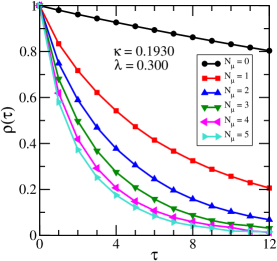
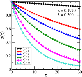
Figure 16: Autocorrelation function $\rho(\tau)$ of the quantity $\langle\Phi(t)\Phi(0)\rangle$ for $t\sim 1/(2a_{s}m)$ and $\Phi(t)=\sum_{xy}\phi(x,y,t)$ against the number of compound sweeps $\tau$, each consisting of one Metropolis sweep followed by $N_{\mu}$ microcanonical sweeps with probability $\mu$ of proposing a change at each site. In both plots, $\mu=1.00$ and $N_{\mu}$ is varied. (a) In the left-hand plot, $t=2a_{t}$ is used with $\kappa=0.1930$ and $\lambda=0.300$ on a $24^{2}\times 48$ isotropic lattice such that the mass gap is about $0.25$; the microcanonical acceptance rate is $0.807$. (b) In the right-hand plot, $t=5a_{t}$ is used with $\kappa=0.1970$ and $\lambda=0.300$ on a $32^{2}\times 96$ isotropic lattice so that the mass gap is about $0.10$; the microcanonical acceptance rate is $0.804$.

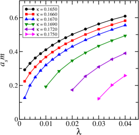
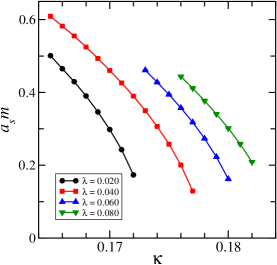
Figure 17: The mass gap $a_{s}m_{\rm gap}$ in $2+1$-dimensional $\phi^{4}$ theory on $24^{3}$ isotropic lattices for various values of the hopping parameter $\kappa$ and the coupling $\lambda$.

Single particle masses on $24^{3}$ isotropic lattices are shown for various values of $\kappa,\lambda$ in Fig. 17. One sees that the mass parameter $m$ in the Lagrangian is no longer the mass of the particle. This $2+1$-dimensional $\phi^{4}$ theory has two phases separated by a line of critical points. For each value of $\lambda$, there exists a critical value $\kappa_{c}(\lambda)$ at which the mass gap goes to zero. The so-called symmetric phase occurs for $\kappa<\kappa_{c}(\lambda)$; in this phase, the $\phi\rightarrow-\phi$ symmetry holds, and $\langle\phi\rangle=0$. The so-called broken phase occurs for $\kappa>\kappa_{c}(\lambda)$; in this phase, the symmetry $\phi\rightarrow-\phi$ of the Lagrangian is spontaneously broken, such that there is a nonzero vacuum expectation value for the field: $\langle\phi\rangle\neq 0$. A somewhat qualitative sketch of the phase boundary is shown in Fig. 18.

Figure 18: The phase boundary for 2+1-dimensional $\phi^{4}$ theory, shown as a critical value $\kappa_{c}(\lambda)$ of the hopping parameter as a function of the coupling $\lambda$. The symmetry $\phi\rightarrow-\phi$ is spontaneously broken above the phase boundary. The theory becomes the Ising model as $\lambda\rightarrow\infty$.

Although the physics of this field theory are very interesting, the focus of these lectures is the Monte Carlo method, which we have already discussed in great detail. In these six lectures, there is inadequate time to study the renormalization group flows of this model, nor to describe the calculational techniques needed to probe the phase transition. Phase transitions only occur in systems having an infinite number of degrees of freedom, requiring an infinite number of lattice sites. Monte Carlo studied must be performed with a finite number of lattice sites out of necessity, so the study of the phase transition requires a few clever tricks. The interested reader is invited to further explore this field theory after these lectures.

6 Monte Carlo calculations in lattice quantum chromodynamics

The field of lattice QCD began with the famous paper of Ken Wilson in 1974[11]. Wilson found a way of formulating QCD on a hypercubic space-time lattice which preserved local gauge invariance, an important property linked to the renormalizability of the theory. In lattice QCD, the quarks reside on the sites, while the gluon field resides on the links between sites. Wilson advocated the use of link variables $U_{\mu}(x)$ which are path-ordered exponentials of the gauge field from one site to its neighbor. In other words, the $U_{\mu}(x)$ are parallel transport matrices. In QCD, the link variables are elements of the group $SU(3)$. For gluons, the path integration involves an eight-dimensional integral on each link, so the path integral has dimension $32N_{x}N_{y}N_{z}N_{t}$. For a $24^{4}$ lattice, the path integral has a dimension near 10.6 million. Of course, the fermion quark fields have to be dealt with, too. The quark fields are Grassmann valued and obey Fermi-Dirac statistics. This introduces major complications into the Monte Carlo updating procedure.

Current Monte Carlo updating methods in pure gauge theories work very well. The best methods are similar to that already described in the $\phi^{4}$ theory. One sweeps through the lattice using either a Metropolis or a heat bath local updating scheme, then sweeps some number of times with an action-preserving local updating method. In some field theories, it is possible to sample the probability density associated with a local update, either using a transformation method or the rejection method. Such a local updating method is called a heat bath[12]. A heat bath method for $SU(2)$ lattice gauge theory was proposed in Ref. creutzheatbath and was later improved in Ref. heatbathsu2. A heat bath method for $SU(3)$ exists[15], but a more efficient pseudo-heatbath method[16] of updating an $SU(3)$ matrix by successive $SU(2)$ subgroups is usually used. Microcanonical (overrelaxation) updating of $SU(2)$ subgroups was proposed in Ref. brown, and a microcanonical procedure for $SU(3)$ is described in Ref. patel. Local microcanonical updating algorithms for general $SU(N)$ gauge theories have been devised in Refs. creutzOR,forcrand.

Monte Carlo updating methods including quarks in lattice QCD are steadily improving. The methods currently used are based on the so-called Hybrid Monte Carlo[21] method and a variant known as RHMC[22]. Fermions present special challenges in terms of formulating them on a lattice and carrying out Monte Carlo calculations. Unfortunately, since my time is nearly up, I will not be able to discuss these issues any further here.

Before concluding, I would like to present the results of two Monte Carlo studies in lattice gauge theory and lattice QCD that I have been personally involved in. An amazing feature of nonabelian gauge theories is that the massless gluons can bind to form rather massive objects known as glueballs. The analog of such particles in electromagnetism would be massive globules of pure light! The mass spectrum of such objects from Ref. glueballs is shown in Fig. 19. States are labeled by $J^{PC}$, where $J$ is the spin, $P$ is the parity, and $C$ is the charge conjugation quantum number. The scale has been set using $r_{0}^{-1}=410(20)$ MeV, where $r_{0}$ is a convenient hadron scale defined in terms of the static quark potential. These results were computed using Cabibbo-Marinari pseudo-heatbath and Creutz microcanonical overrelaxation. A $24\times 24$ correlation matrix was used in each symmetry channel. The mass of the lowest-lying scalar glueball is the only particle mass that I know of that has a bounty on its head: the Clay Mathematics Institute will pay $1 million for a mathematical proof that this mass is nonzero.

Figure 19: The mass spectrum of glueballs in the pure $SU(3)$ gauge theory from Ref glueballs. The masses are given in terms of the hadronic scale $r_{0}$ along the left vertical axis and in terms of GeV along the right vertical axis (assuming $r_{0}^{-1}=410$ MeV). The mass uncertainties indicated by the vertical extents of the boxes do not include the uncertainty in setting $r_{0}$. The locations of states whose interpretation requires further study are indicated by the dashed hollow boxes.

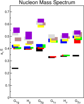
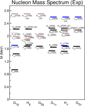
Figure 20: (Left) An exploratory first computation of the nucleon spectrum from 200 quenched configurations on a $12^{3}\times 48$ anisotropic lattice using the Wilson gauge and quark actions with $a_{s}\sim 0.1$ fm, $a_{s}/a_{t}\sim 3.0$ and $m_{\pi}\sim 700$ MeV. The results are from Ref. lichtl2006. (Right) The currently known spectrum from experiment. Black denotes four-star states, blue denotes three-star states, tan denotes two-star states, and gray denotes a one-star state.

I am currently a member of a collaboration of lattice QCD theorists known as the Lattice Hadron Physics Collaboration (LHPC). One of our current goals is to use the Monte Carlo method to predict the baryon and meson spectrum of QCD. Our plans on how we intend to accomplish this are outlined in Ref. baryons. We have recently completed exploratory studies[24] on small anisotropic lattices in the quenched approximation to QCD (ignoring quark loops) at relatively large quark masses. These studies demonstrated our ability to isolate up to nine energy eigenvalues from our correlation functions. The spectrum of isospin $I=1/2$ states, albeit at an unphysically large quark mass corresponding to $m_{\pi}\simeq 700~{}{\rm MeV}$, is shown as the left-hand panel in Fig. 20. The right-hand panel shows the experimental spectrum, with states assigned according to the irreducible representations of the cubic group; even in this quenched calculation, at unphysical pion masses, there are tantalizing suggestions of the existence of a band of negative-parity states well separated from the higher excitations, as observed experimentally. These calculations are ongoing.

7 Conclusion

This series of six lectures was an introduction to using the Monte Carlo method to carry out nonperturbative studies in quantum field theories. First, the path integral method in nonrelativistic quantum mechanics was reviewed and several simple examples were studied: a free particle in one dimension, the one-dimensional infinite square well, a free particle in one dimension with periodic boundary conditions, and the one-dimensional simple harmonic oscillator. The extraction of observables from correlation functions or vacuum expectation values was discussed, and the evaluation of these correlation functions using ratios of path integrals was described, introducing Wick rotations to imaginary time.

A major portion of this series of lectures was then devoted to the evaluation of path integrals in the imaginary time formalism using the Monte Carlo method with Markov chains. After a brief review of probability theory, the law of large numbers and the central limit theorem were used to justify simple Monte Carlo integration. However, the estimation of path integrals with sufficient accuracy required the need for clever importance sampling, which led to the use of stationary stochastic processes, and in particular, ergodic Markov chains. Several properties of Markov chains were discussed and proven, particularly the fundamental limit theorem for ergodic Markov chains. The Metropolis-Hastings method of constructing a Markov chain was described.

Next, the one-dimensional simple harmonic oscillator was studied using the Metropolis method. One of the simplest quantum field theories, a real scalar field theory with a $\phi^{4}$ interaction in three space-time dimensions, was then studied. The Metropolis method was seen to be plagued by strong autocorrelations. An action-preserving (microcanonical) updating method was described, and its effectiveness in reducing autocorrelations was demonstrated. The extraction of stationary-state energies was detailed, introducing correlated-$\chi^{2}$ fitting, as well as jackknife and bootstrap error estimates. The lectures concluded with some comments and results from lattice QCD.

In addition to the references already cited, see Ref. snell,ross,billingsley for an introduction to probability, Refs. parzen,prabhu for more details concerning stochastic processes, and Ref. montvay for a very good textbook on quantum fields on a lattice.

This work was supported by the U.S. National Science Foundation through grant PHY-0354982. I would especially like to thank Robert Edwards, Jimmy Juge, Julius Kuti, Adam Lichtl, Mike Peardon, and David Richards for their helpful comments and suggestions.

References

- [1] R. Feynman, Rev. Mod. Phys. 20, p. 367 (1948).
- [2] M. Goodman, Am. Jour. Phys 49, p. 9 (1981).
- [3] N. Etemadi, Prob. Theory and Related Fields 55, p. 119 (1981).
-
[4]
M. Matsumoto and T. Nishimura, ACM Trans. on Modeling and Computer
Simulation 8, p. 3 (1998),
http://www.math.sci.hiroshima-u.ac.jp/~m-mat/MT/emt.html. - [5] W. Hoeffding and H. Robbins, Duke Math. Journal 15, p. 773 (1948).
- [6] T. Anderson, The Statistical Analysis of Time Series (Wiley, New York, 1971).
- [7] W. Feller, An Introduction to Probability Theory and Its Applications, Vol. I. (Wiley, New York, 1967).
- [8] S. Karlin and H. Taylor, A First Course in Stochastic Processes (Academic Press, New York, 1975).
- [9] N. Metropolis, A. Rosenbluth, M. Rosenbluth, A. Teller and E. Teller, J. Chem. Phys. 21, p. 1087 (1953).
- [10] W. Hastings, Biometrika 57, p. 97 (1970).
- [11] K. Wilson, Phys. Rev. D 10, p. 2445 (1974).
- [12] C. Yang, Proceedings of Symposia in Applied Mathematics, Vol. XV (American Mathematical Society, Providence, RI, 1963), Providence, RI, p. 351.
- [13] M. Creutz, Phys. Rev. D 21, p. 2308 (1980).
- [14] A. Kennedy and B. Pendleton, Phys. Lett. B 156, p. 393 (1985).
- [15] E. Pietarinen, Nucl. Phys. B 190, p. 349 (1981).
- [16] N. Cabibbo and E. Marinari, Phys. Lett. B 119, p. 387 (1982).
- [17] F. Brown and T. Woch, Phys. Rev. Lett. 58, p. 2394 (1987).
- [18] R. Gupta, G. Guralnik, A. Patel, T. Warnock and C. Zemach, Phys. Rev. Lett. 53, p. 1721 (1984).
- [19] M. Creutz, Phys. Rev. D 36, p. 515 (1987).
- [20] P. de Forcrand and O. Jahn, in the proceedings of the 3rd International Workshop on Numerical Analysis and Lattice QCD, p. 67, 2003 [arXiv:hep-lat/0503041].
- [21] S. Duane, A. Kennedy, B. Pendleton and D. Roweth, Phys. Lett. B 195, p. 216 (1987).
- [22] M. Clark, A. Kennedy and Z. Sroczynski, Nucl. Phys. B (Proc. Suppl.) 140, p. 835 (2005), [arXiv:hep-lat/0409133].
- [23] C. Morningstar and M. Peardon, Phys. Rev. D 60, p. 034509 (1999).
- [24] A. Lichtl, Quantum operator design for lattice baryon spectroscopy, PhD thesis, Carnegie Mellon University, 2006 (with the LHP Collaboration) [arXiv:hep-lat/0609019].
- [25] S. Basak, R. Edwards, G. Fleming, U. Heller, C. Morningstar, D. Richards, I. Sato and S. Wallace, Phys. Rev. D 72, p. 094506 (2005).
- [26] C. Grinstead and J. Snell, Introduction to Probability (American Mathematical Society, Providence, RI, 2003).
- [27] S. Ross, A First Course in Probability (Prentice Hall, New Jersey, 1998).
- [28] P. Billingsley, Probability and Measure (Wiley, New York, 1986).
- [29] E. Parzen, Stochastic Processes (Holden-Day, San Francisco, 1962).
- [30] N. Prabhu, Stochastic Processes (Macmillan, New York, 1965).
- [31] I. Montvay and G. Münster, Quantum Fields on a Lattice (Cambridge Press, New York, 1994).