Neutron electric dipole moment with external electric field method in lattice QCD

Abstract

We discuss a possibility that the Neutron Electric Dipole Moment (NEDM) can be calculated in lattice QCD simulations in the presence of the CP violating $\theta$ term. In this paper we measure the energy difference between spin-up and spin-down states of the neutron in the presence of an uniform and static external electric field. We first test this method in quenched QCD with the RG improved gauge action on a $16^{3}\times 32$ lattice at $a^{-1}\simeq$ 2 GeV, employing two different lattice fermion formulations, the domain-wall fermion and the clover fermion for quarks, at relatively heavy quark mass $(m_{PS}/m_{V}\simeq 0.85)$. We obtain non-zero values of NEDM from calculations with both fermion formulations. We next consider some systematic uncertainties of our method for NEDM, using $24^{3}\times 32$ lattice at the same lattice spacing only with the clover fermion. We finally investigate the quark mass dependence of NEDM and observe a non-vanishing behavior of NEDM toward the chiral limit. We interpret this behavior as a manifestation of the pathology in the quenched approximation.

I Introduction

Discrete symmetries, such as parity (P), charge conjugation (C) and time-reversal (T), have played important roles to establish the structure of the standard model. One of the most famous examples is CP violation which led to three generations of quarks and leptonsKM .

In the strong interaction, the most strict constraint on violation of P and T symmetries comes from the measurement of the electric dipole moment (EDM) for neutron (NEDM) and proton (PEDM). The current upper bound is given by

$$|d_{N}|<6.3\times 10^{-13}\,\,e\cdot\textrm{fm}\,\textrm{(90\%C.L.)}\,$$ (1)

for neutron from a Larmor frequency measurement with ultra-cold neutron (UCN)Harris , and

$$|d_{N}|<5.4\times 10^{-11}\,\,e\cdot\textrm{fm}$$ (2)

for protonDmitriev , which is estimated indirectly from EDM of mercury atom ${}^{199}\rm{H}_{\rm{g}}$ given by $d_{\rm atom}({}^{199}\rm{H}_{\rm{g}})<2.1\times 10^{-15}\,e\cdot\rm{fm}\,\textrm{(95\% C.L.)}$Romalis .

On the other hand, QCD allows a gauge invariant, renormalizable, and CP odd $\theta$ term,

$$i\frac{\theta}{32\pi^{2}}\int d^{4}x\,\widetilde{G}_{\mu\nu}(x)G_{\mu\nu}(x),\qquad\widetilde{G}_{\mu\nu}(x)=\frac{1}{4}\epsilon_{\mu\nu\alpha\beta}G_{\alpha\beta}(x)$$ (3)

in Euclidean space-time with $G_{\mu\nu}$ which is the field strength of gluon. Some model estimationsCrewther ; Vecchia yield

$$|d_{N}|\sim\theta\times O(10^{-2}\sim 10^{-3})\,e\cdot{\rm fm},$$ (4)

which leads to a bound $\theta\leq O(10^{-10})$. Hence $\theta$ must be very small or even may vanish in QCD.

Smallness of $\theta$ in the QCD sector, however, is not protected in the presence of the electroweak sector of the standard model, where the quark mass matrix, arising from Yukawa couplings to the Higgs field, may be written as

$$\bar{\psi}^{R}_{i}(x)M_{ij}\psi^{L}_{j}(x)+\bar{\psi}^{L}_{i}(x)M^{{\dagger}}_{ij}\psi^{R}_{j}(x),$$ (5)

where $\psi^{L}$ and $\psi^{R}$ represent left and right handed quark fields with flavor indices $i,j$. Diagonalizing the mass matrix and making it real, the parameter $\theta$ becomes

$$\theta=\theta_{\rm QCD}+\arg\det M,$$ (6)

where $\theta_{\rm QCD}$ is the original $\theta$ parameter in QCD. Therefore, $\theta_{\rm QCD}$ and $\arg\det M$ contributions have to cancel out to the precise degree that the stringent experimental upper bound on NEDM is satisfied. In either of the two cases, it seems necessary to explain why Nature chooses such a small value for $\theta$; this is the “strong CP problem”. One of the most attractive explanations proposed so far is the Peccei-Quinn mechanismPeccei . Unfortunately, the axion, a new particle predicted by this mechanism, has not been experimentally observed so far.

Present theoretical estimations of NEDM vary in magnitude among different models such as current algebraCrewther , chiral perturbation theoryVecchia ; Aoki_Hatsuda ; Cheng ; Pich , and QCD sum rulePospelov ; Chan (see also Pospelov:05 ). While these crude estimations of $|d_{N}|/\theta$ already convince the smallness of $\theta$, a theoretically reliable and accurate estimation for NEDM will be required to determine the value of $\theta$, if a non-zero value of NEDM is observed in future experiments. Lattice QCD calculations provide a first-principle method for this task. Indeed more than fifteen years ago, the first attempt was made to estimate NEDM in a quenched lattice QCD simulationAoki1 . Reliable signal of NEDM could not be obtained at this timeAoki2 . Since then, no lattice calculation of NEDM have been attempted until recently. In the last year, new approach has been presented for this problem. Ref.Shitani_form ; Shintani_wE ; Shintani_wE2 proposed a formulation to extract the CP-odd electromagnetic form factor of nucleon from certain lattice correlation functions. NEDM can be extracted from this form factor in the zero momentum transfer limit. Applying this formulation in a quenched calculation with domain-wall quarks, a non-zero value for the CP-odd form factor of nucleon was obtained at one value of non-zero momentum. Based on this formulation, the same form factor has been calculated on gauge configurations generated by $N_{f}=2$ dynamical domain-wall QCD at several non-zero momentaRBC . The value of NEDM after the zero momentum extrapolation, however, is consistent with zero within the large statistical error in this calculation.

The results mentioned above suggest that, while it is possible to obtain signals for the CP odd form factor at fixed and small value of momentum, it is numerically difficult to carry out a statistically controlled extrapolation of the form factor to the zero momentum limit to extract the value of EDM. Therefore, in this paper, we investigate another method to calculate the value of EDM directly without momentum extrapolation. In this method, introducing a constant uniform electric field $\vec{E}$, we measure the energy difference between spin-up and spin-down components of the nucleon in the presence of the $\theta$ term Aoki1 . If the electric field is small enough, the leading contribution to the energy difference is given by $d_{N}\vec{S}\cdot\vec{E}$ with neutron spin $\vec{S}$ and electric field $\vec{E}$. Therefore EDM can be directly extracted without momentum extrapolation. The most difficult part of this calculation is to reweight the nucleon propagator on a given gauge configuration with the factor $e^{i\theta Q}$, where $Q$ is the topological charge of the configuration. We may control this reweighting by taking a small value of $\theta$. Another difficulty is that our electric field breaks periodicity in the time direction, generating large field at the time boundary. We should investigate influences of the large electric field at the boundary to EDM signals.

We check the ability of this method in the quenched approximation at a heavy quark mass. We employ two fermion formulations, domain-wall fermion having chiral symmetry and clover fermion with explicitly broken chiral symmetry, in order to investigate possible dependence of EDM signals on the aspect of chiral symmetry of fermion formulations. Our study have revealed that the quality of EDM signals is not very sensitive to fermion formulations. Therefore we have employed the clover fermion, which requires much less computational cost than the domain-wall fermion, to study various systematics of EDM such as the volume dependence, the boundary effect and the quark mass dependence within the quenched approximation.

This paper is organized as following. In sec. II we explain the definition of EDM and our method to extract EDM from nucleon propagators. Simulation details of our lattice calculation are summarized in sec. III. In sec. IV we show numerical results with both domain-wall and clover fermion at heavy quark mass on a $16^{3}\times 32$ lattice. We then investigate the finite size effect and the boundary effect on a $24^{3}\times 32$ lattice with the clover fermion. In V we systematically study the quark mass dependence of EDM using the larger lattice with the clover fermion. A summary and discussion is given in the last section VI.

II EDM with electric field

In our previous workShitani_form , we defined NEDM from the CP-odd electromagnetic form factor, $F_{3}$, in the zero momentum transfer limit. In the actual calculation, however, it is not so easy to change the momentum transfer, since the momentum is quantized as $\displaystyle p=n\frac{\pi}{L}$ on a finite spatial length of $L$. In the case of large $p$ with $n=2,3,\cdots$ at small $L$, statistical errors are large, while a smaller $p$ with $n=2,3,\cdots$, which has a better signal, requires a larger lattice size $L$. In both cases, the calculation becomes more difficult for larger momentum at $n=2,3\cdots$ than for the smallest momentum at $n=1$. In addition, the correct distribution of the topological charge is essentially important for the NEDM calculation. Since the width of the distribution of topological charge increases linearly with the volume, larger volume calculations require more statistics than the small volume ones, contrary to other observables.

The difficulties for the extrapolation to the zero momentum transfer limit mentioned above are our motivations to consider a different method for the NEDM calculation with which we can avoid the momentum extrapolation. In this section we introduce our new approach for the lattice QCD calculation of NEDM.

II.1 Formulation

In ref. Aoki1 , NEDM is defined through the energy change of the neutron state in the presence of an external electric field, similarly to the magnetic moment defined from that in the magnetic field. If a static and uniform electric field exists in a CP-violating system, the electric dipole moment(EDM) appears in the Hamiltonian as the interaction term between spin $\vec{S}$ of particle and electric field $\vec{E}$:

$$\delta H_{\rm CP}=d_{N}(\theta){\vec{S}}\cdot\vec{E}+O((\vec{E})^{3})$$ (7)

where $d_{N}(\theta)$ represents the EDM. In order to extract EDM we consider the energy difference of nucleon states for opposite spins in the external electric field:

$$m^{\theta}_{\vec{s}}(\vec{E})-m^{\theta}_{-\vec{s}}(\vec{E})=2d_{N}(\theta){\vec{S}}\cdot\vec{E}+O((\vec{E})^{3}),$$ (8)

where $m^{\theta}_{\pm\vec{s}}(\vec{E})$ denotes the energy of nucleon whose spin vector is $\pm\vec{S}$ in the presence of the electric field $\vec{E}$. Therefore we can extract $d_{N}(\theta)$ from the nucleon propagators for two different spin states at zero momentum only, avoiding difficult calculations at non-zero momenta.

For small $\theta$ we can expand $d_{N}(\theta)$ as

$$d_{N}(\theta)=d_{N}\theta+\mathcal{O}(\theta^{3}).$$ (9)

We will check that higher order contributions at $\mathcal{O}(\theta^{3})$ are negligibly small. Hereafter we represent $d_{N}$ as the leading order of EDM.

II.2 Methodology on the lattice

A static and uniform electric field is represented by the spatial gauge potential as

$$A_{i}(x)=E_{i}^{\rm Euclid}t$$ (10)

where $E_{i}^{\rm Euclid}$ is the constant electric field in Euclidean space. A non-zero NEDM could be detected from the oscillating behavior of the neutron propagator. Since NEDM is expected to be small, it is numerically very difficult to measure such a small oscillation. On the other hand, if we employ a static and uniform electric field in Minkovski space as

$$A_{i}(x)=-iE_{i}^{\rm Minkov}t,$$ (11)

the oscillation turns into an exponential behavior, which is easier to measure. Therefore we introduce a static and uniform electric field in Minkovski space as an external field into lattice QCD, by replacing the spatial link variables as

$$U_{i}(x)\longrightarrow\widetilde{U}_{i}(x;E^{\rm Minkov}_{i}) = e^{q_{e}E^{\rm Minkov}_{i}t}U_{i}(x),$$

$$U^{-1}_{i}(x)\longrightarrow\widetilde{U}_{i}^{-1}(x;E^{\rm Minkov}_{i}) = e^{-q_{e}E^{\rm Minkov}_{i}t}U^{-1}_{i}(x),$$ (12)

where $q_{e}$ denotes the quark charge, $2/3$ for up quark and $-1/3$ for down quark. Hereafter we suppress the superscript of the constant electric field $E_{i}$ in Minkovski space for simplicity.

An obvious problem here is that the Minkovski electric field $E$ breaks the periodic boundary condition in the temporal direction:

$$U_{i}(t+T,\vec{x}) = U_{i}(t,\vec{x}),$$ (13)

$$\widetilde{U}_{i}(t+T,\vec{x};E_{i}) = e^{q_{e}E_{i}T}\widetilde{U}_{i}(t,\vec{x};E_{i})\neq\widetilde{U}_{i}(t,\vec{x};E_{i})$$ (14)

where $T$ is the size of the temporal direction. This generates an effective electric field, defined by $E_{i}(t)=\frac{A_{i}(t+1)-A_{i}(t-1)}{2}$, as

$$E_{i}(t)=\left\{\begin{array}[]{ll}E_{i}&t=2,3,\cdots,T-1\\ -E_{i}\frac{T-2}{2}&t=1,T\\ \end{array}\right..$$ (15)

Therefore the electric field is no more constant near the boundary between $t=1$ and $t=T$. In order to avoid the effect of this non-uniform electric field to the EDM signal, we have to take $E_{i}$ as small as possible. In any case a small value of $E_{i}$ is necessary to neglect $O((\vec{E})^{3})$ terms in (7).

In our calculation gauge configurations are generated by the usual lattice QCD action without $E$ and $\theta$. After inserting the electric field to gauge configurations we calculate quark propagators for flavor $u$ and $d$ separately, in addition to the normal one with $E_{i}=0$, which is used to remove a fake signal at $E_{i}=0$ caused by statistical fluctuations. The total number of solvers for quark propagators is three for each configuration. From quark propagators we construct the nucleon propagator with the $\theta$ term as

$$\langle N_{\alpha}\bar{N}_{\beta}\rangle_{\theta}(\vec{E},t)=\langle N_{\alpha}(t)\bar{N}_{\alpha}(0)e^{i\theta Q}\rangle_{\vec{E}}$$ (16)

where $\langle{\cal O}\rangle_{\vec{E}}$ represents the vacuum expectation value of ${\cal O}$ with $\vec{E}$ but without the $\theta$ term. Here we use the re-weighting method with the complex weight factor $e^{i\theta Q}$. In order to obtain good signals, a large overlap of gauge ensembles between $\theta=0$ and $\theta\not=0$ as well as the correct distribution of the topological charge are required. Taking a small value of $\theta$ as long as we get a signal helps for the large overlap, while we have to simply accumulate an enough number of configurations for the correct distribution of the topological charge.

In the presence of the uniform and static electric field, the upper components of the nucleon propagator at zero spatial momentum take the following form for $\alpha,\,\beta=1,2$Aoki3 :

$$\langle N_{\alpha}\bar{N}_{\beta}\rangle_{\theta}(\vec{E},t) = Z^{\prime}_{N}{}^{\theta}(E^{2}\equiv\vec{E}\cdot\vec{E})\Big{[}\left(1+A_{N}(\theta,E^{2})\vec{\sigma}\cdot\vec{E}\right)$$ (17)

$$\times \exp\big{(}-m_{N}^{\theta}(E^{2})t-\frac{d_{N}(\theta,E^{2})}{2}\vec{\sigma}\cdot\vec{E}t\big{)}\Big{]}_{\alpha\beta}+\cdots,$$

where the EDM $d_{N}(\theta,E^{2})$ and the spin-dependent amplitude $A_{N}(\theta,E^{2})$ are odd in $\theta$, while the spin-independent energy $m^{\theta}(E^{2})$ and an overall amplitude $Z^{\prime}_{N}{}^{\theta}(E^{2})$ are even in $\theta$. Here dots denote contributions from excited states.

To extract EDM we construct the ratio of nucleon propagators between different spinor components. For $\vec{E}=(0,0,E)$ we consider the following ratio:

$$R^{\rm naive}_{3}(E,t;\theta)=\frac{\langle N_{1}\bar{N}_{1}\rangle_{\theta}((0,0,E),t)}{\langle N_{2}\bar{N}_{2}\rangle_{\theta}((0,0,E),t)}=\frac{1+A_{N}(\theta,E^{2})E}{1-A_{N}(\theta,E^{2})E}\exp[-d_{N}\theta Et+\mathcal{O}(\theta^{3}E,\theta E^{3})],$$ (18)

where we use eq. (17) for the second equality. Similarly for $\vec{E}=(E,0,0)$ and $(0,E,0)$, we obtain

$$R^{\rm naive}_{1}(E,t;\theta) = \frac{\langle N_{1}\bar{N}_{1}\rangle_{\theta}+\langle N_{1}\bar{N}_{2}\rangle_{\theta}+\langle N_{2}\bar{N}_{1}\rangle_{\theta}+\langle N_{2}\bar{N}_{2}\rangle_{\theta}}{\langle N_{1}\bar{N}_{1}\rangle_{\theta}-\langle N_{1}\bar{N}_{2}\rangle_{\theta}-\langle N_{2}\bar{N}_{1}\rangle_{\theta}+\langle N_{2}\bar{N}_{2}\rangle_{\theta}}((E,0,0),t)$$

$$= \frac{1+A_{N}(\theta,E^{2})E}{1-A_{N}(\theta,E^{2})E}\exp[-d_{N}\theta Et+\mathcal{O}(\theta^{3}E,\theta E^{3})],$$

$$R^{\rm naive}_{2}(E,t;\theta) = \frac{\langle N_{1}\bar{N}_{1}\rangle_{\theta}+i\langle N_{1}\bar{N}_{2}\rangle_{\theta}-i\langle N_{2}\bar{N}_{1}\rangle_{\theta}+\langle N_{2}\bar{N}_{2}\rangle_{\theta}}{\langle N_{1}\bar{N}_{1}\rangle_{\theta}-i\langle N_{1}\bar{N}_{2}\rangle_{\theta}+i\langle N_{2}\bar{N}_{1}\rangle_{\theta}+\langle N_{2}\bar{N}_{2}\rangle_{\theta}}((0,E,0),t)$$

$$= \frac{1+A_{N}(\theta,E^{2})E}{1-A_{N}(\theta,E^{2})E}\exp[-d_{N}\theta Et+\mathcal{O}(\theta^{3}E,\theta E^{3})].$$

We can average over the ratio in three directions to increase statistics, if necessary.

In order to remove the spurious contribution $m^{\theta}_{\vec{s}}(0)-m^{\theta}_{-\vec{s}}(0)$, which must vanish for infinite statistics, we consider a double ratio defined by

$$R_{i}(E,t;\theta) = \left[\frac{R^{\rm naive}_{i}(E,t;\theta)}{R^{\rm naive}_{i}(0,t;\theta)}\right],$$ (21)

$$\ln\left[\frac{R_{i}(E,t;\theta)}{R_{i}(E,t+1;\theta)}\right] = [m^{\theta}_{\vec{s}}(E_{i})-m^{\theta}_{\vec{s}}(0)]-[m^{\theta}_{-\vec{s}}(E_{i})-m^{\theta}_{-\vec{s}}(0)]$$ (22)

$$= d_{N}\theta E+\mathcal{O}(\theta^{3}E,\theta E^{3}).$$ (23)

We can improve the EDM signal further, removing the contribution at $\theta=0$, which also vanish for infinite statistics, by a triple ratio as

$$R_{i}^{({\rm w/o\,\theta=0})}(E,t;\theta)=\frac{R_{i}(E,t;\theta)}{R_{i}(E,t;\theta=0)}\simeq\frac{1+\theta A_{N}^{1}(E^{2})E}{1-\theta A_{N}^{1}(E^{2})E}\exp[d_{N}\theta Et],$$ (24)

where we used an expansion $A_{N}(\theta,E^{2})=\theta A_{N}^{1}(E^{2})+\mathcal{O}(\theta^{3})$, and we finally subtract the spurious contribution even in $E$ by a quadruple ratio as

$$R_{i}^{\rm corr}(E,t;\theta) = \frac{R^{({\rm w/o\,\theta=0})}_{i}(E,t;\theta)}{R^{({\rm w/o\,\theta=0})}_{i}(-E,t;\theta)}$$ (25)

$$= \frac{R_{i}^{\rm naive}(E,t;\theta)}{R_{i}^{\rm naive}(-E,t;\theta)}\frac{R_{i}^{\rm naive}(-E,t;\theta=0)}{R_{i}^{\rm naive}(E,t;\theta=0)}$$

$$\simeq \left(\frac{1+\theta A_{N}^{1}(E^{2})E}{1-\theta A_{N}^{1}(E^{2})E}\right)^{2}\exp[2d_{N}\theta Et],$$

where the second equality tell us that this is indeed a triple ratio since $\vec{E}=0$ contributions are canceled identically. We finally extract EDM from the exponential fit to $R_{i}^{\rm corr}(E,t;\theta)$ over some time range, determined by the behavior of the effective EDM:

$$2d_{N}\theta E=\ln\left[\frac{R^{\rm corr}_{i}(E,t;\theta)}{R^{\rm corr}_{i}(E,t+1;\theta)}\right],\quad i=1,2,3.$$ (26)

III Simulation details

III.1 Simulation parameters

In our study we employ gauge configurations generated by the RG improved gauge action at $\beta=2.6$ in the quenched approximation, which corresponds to $a^{-1}=1.902(50)$ GeV from the string tension $\sigma$ assuming $\sigma=(440\,\textrm{MeV}^{2})$Okamoto .

For the quark action, we employ the domain-wall fermion on a $16^{3}\times 32$ lattice with the fifth length $N_{s}=16$ and the domain-wall height $M=1.8$. These parameters are identical to those in the previous EDM form factor calculation. We however take a heavier quark mass, $m_{f}=0.12$, which corresponds to $m_{N}a=1.113(2)$ and $m_{PS}/m_{V}\simeq 0.88$, than the one in the previous calculation, in order to reduce the computational cost, since our main motivation in this calculation is to see whether the EDM signal can be obtained by this method. As shown in the next section we have indeed obtained the EDM signal after accumulating 1000 configurations at this heavier quark mass.

We also investigate whether the EDM signal can be obtained by this method with the clover fermion. The EDM calculation with this fermion has the advantage that the computational cost is roughly $N_{s}$ times smaller than the cost of the domain-wall fermion so that systematic studies such as volume or quark mass dependences can be performed more easily. Moreover we can employ the $N_{f}=2$ and $2+1$ flavor dynamical configurations already generated with the clover quark action at several sea quark masses and lattice spacingscppacs ; cppacs-jlqcd ; pacscs in future studies. We calculate the EDM on the same $16^{3}\times 32$ configurations, using the clover fermion with $c_{SW}=1.340$, the tadpole improved value of the clover coefficient determined from

$$c_{SW}=\Big{[}\sum_{x,\mu<\nu}P_{\mu\nu}(x)\Big{]}^{-3/4}=(1-0.8412\beta^{-1})^{-1/4}.$$ (27)

In order to obtain a similar nucleon mass, we use the hopping parameter $\kappa=0.1320$, corresponding to $m_{N}a=1.020(2)$ and $m_{PS}/m_{V}\simeq 0.85$.

Since, as will be shown later, the EDM signal can be successfully obtained with the clover fermions, we investigate the volume dependence of the EDM signal using a $24^{3}\times 32$ lattice. Furthermore the quark mass dependence of the EDM is calculated with this fermion on this larger volume.

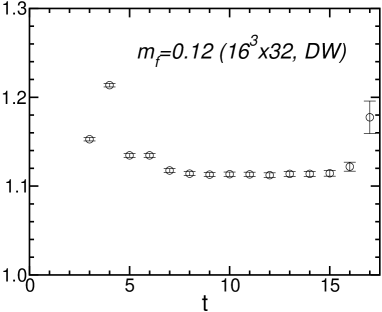
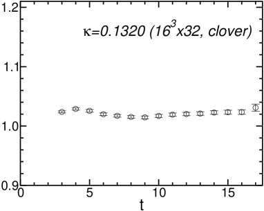
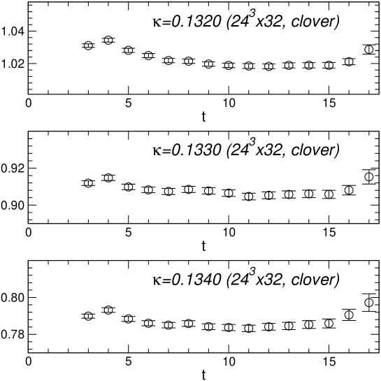
Figure 1: The effective mass plot for nucleon with domain-wall fermion at $m_{f}=0.12$ (top-left), clover fermion at $\kappa=0.1320$ (top-right) on a $16^{3}\times 32$ lattice and clover fermion at various quark masses (bottom) on a $24^{3}\times 32$.

For the calculation of quark propagators we employ the smeared source of the form that $f(r)=Ae^{-Br}$ where $r=|\vec{x}-\vec{x}_{\rm src}|$ with the source point $\vec{x}_{\rm src}=(8,8,8)$ on $16^{3}$ and $(12,12,12)$ on $24^{3}$ spatial lattice, after the Coulomb gauge fixing is applied to gauge configurations. We mainly take $t_{\rm src}=1$ as the time slice of the smeared source. In order to check the effect of the non-uniform electric field near $t=1$ and $T$, we also calculate the EDM with $t_{\rm src}=8$, using the clover fermion on a $24^{3}\times 32$ lattice. Effective mass plots of nucleon in various cases are given in Fig. 1. We observe the plateau at $t\geq 7$ for the domain-wall fermion and the clover fermion at heaviest quark mass, while plateau appears at $t\geq 6$ for the clover fermion at lighter quark masses.

In our calculation we mainly take $\vec{E}=(0,0,E)$ with $E=\pm 0.004$. As exceptions, $E=\pm 0.002$ is employed on a $16^{3}\times 32$ lattice with the domain-wall fermion to investigate the $E$ dependence of the EDM signal, and $(E,0,0)$ and $(0,E,0)$ are used on a $24^{3}\times 32$ lattice with the clover fermion at heaviest quark mass to check the consistency and to increase statistics. Although we can easily change the value of $\theta$ by reweighting, we fix $\theta=0.1$ in our calculation, except $\theta=0.05$ and $0.2$ on a $16^{3}\times 32$ lattice with the domain-wall fermion to investigate the $\theta$ dependence of the EDM signal.

Parameters of fermion actions in various cases are summarized in Table 1.

III.2 Topological charge

The topological charge using the $\mathcal{O}(a^{2})$ improved definitionimpQ is measured on each configuration after 20 cooling steps.

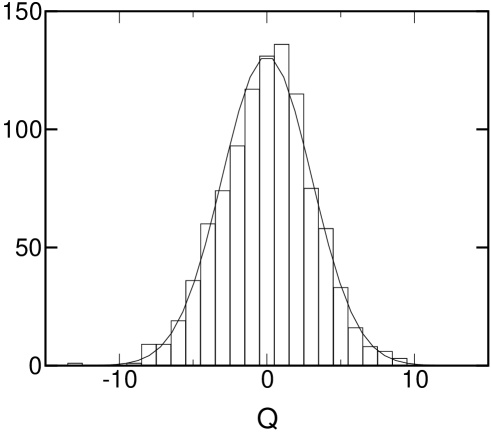
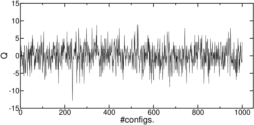
Figure 2: (top) Histogram of topological charge improved by $\mathcal{O}(a^{2})$ after 20 cooling steps. The solid line denotes the expected gaussian distribution from $\sigma=\sqrt{\langle Q^{2}\rangle-\langle Q\rangle^{2}}$. (bottom) The topological charge in each configuration.

On a $16^{3}\times 32$ lattice we accumulate 1000 configurations. In Fig. 2 we present the histogram of the topological charge, which is consistent with gaussian distribution. The symmetry of the distribution is measured by the average of $Q$, which is consistent with zero within error: $\langle Q\rangle=-0.002(97)$. If the gaussian distribution is assumed, its width $\sigma$ is given by $\langle Q^{2}\rangle=9.37(44)$. On this lattice size 1000 configurations seem enough to give a reasonable distribution of the topological charge.

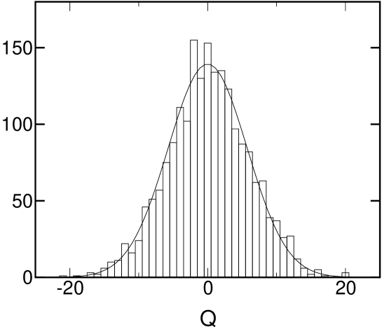
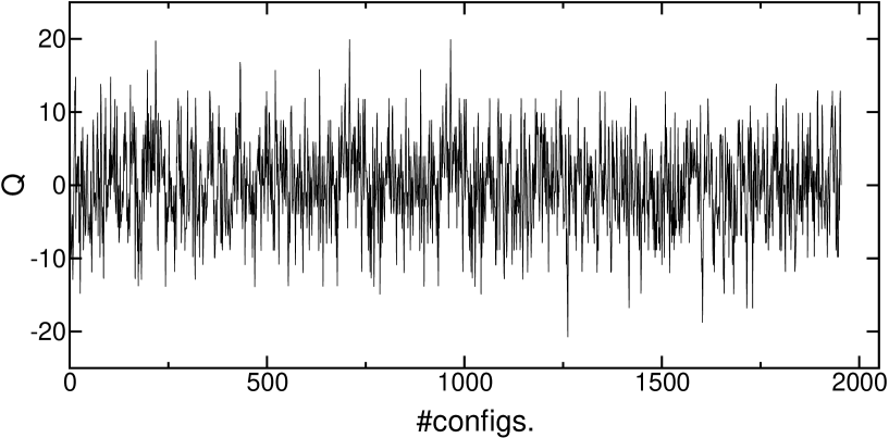
Figure 3: (top) Histogram of the topological charge in $24^{3}\times 32$ lattice and (bottom) the topological charge in each configuration as shown in Fig. 2.

On a larger volume of a $24^{3}\times 32$ lattice, we accumulate nearly 2000 configurations since $\langle Q^{2}\rangle$, thus the width of the distribution of $Q$, increases linearly in volume. In Fig. 3, we show the histogram of $Q$, which looks reasonable, namely sufficiently symmetric and close to gaussian. We find $\langle Q\rangle=0.15(13)$ and $\langle Q^{2}\rangle=33.6(1.1)$.

IV EDM signal and Systematics

In this section, we show numerical results for nucleon EDM signals with the external electric field method. We investigate several systematics of the EDM signal such as dependences on the fermion action, the volume, $E$, $\theta$, $t_{\rm src}$ and the direction of $\vec{E}$.

IV.1 Comparison between domain-wall and clover fermions

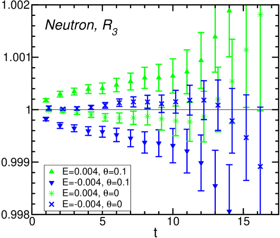
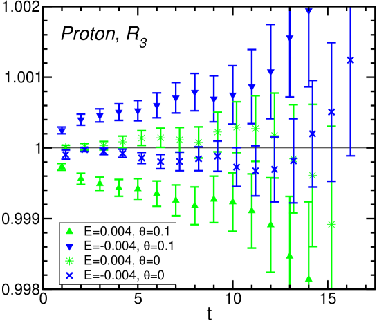
Figure 4: The time behavior of $R_{3}(E,t;\theta)$ in $E=\pm 0.004,\,\theta=0.1$ and $E=0.004,\,\theta=0$ with domain-wall fermion. (Top) neutron case, (bottom) proton case.

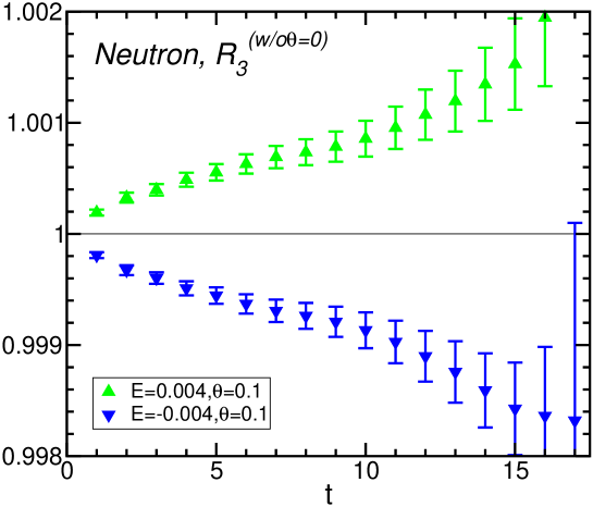
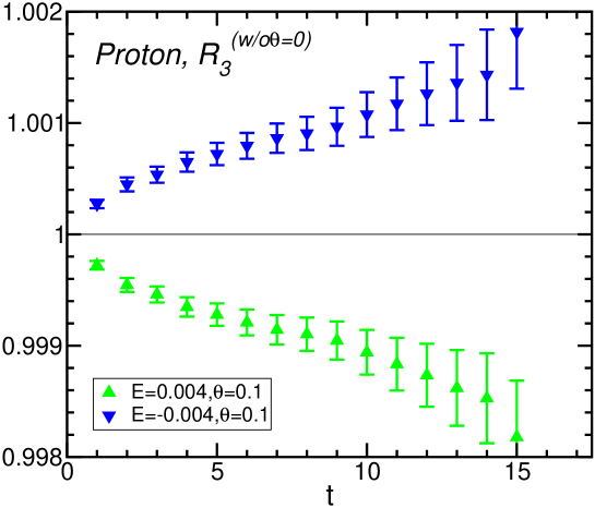
Figure 5: The time behavior of $R^{(\rm w/o\theta=0)}_{3}(E,t;\theta)$ in $E=\pm 0.004,\,\theta=0.1$ with domain-wall fermion. (Top) neutron case, (bottom) proton case.

We first consider the case of the domain-wall fermion on a $16^{3}\times 24$ lattice. In Fig. 4 we plot the double ratio $R_{3}(E,t;\theta)$ as a function of $t$ at $(E,\theta)=(\pm 4.0\times 10^{-3},0.1)$ and $(E,\theta)=(\pm 4.0\times 10^{-3},\theta=0)$, for both neutron and proton. The star symbols in Fig. 4, representing the time dependence of $R_{3}(\pm E,t;\theta=0)$, are consistent with unity within errors at both $\pm E$. This confirms the expected behavior that the exponential part of $R_{3}(E,t;\theta)$ vanishes at $\theta=0$. For non-zero $\theta$, on the other hand, deviations of $R_{3}(E,t;\theta)$ from unity show up beyond errors and they increases as $t$ increases. Moreover the sign of deviations depends on the sign of $E$. All these behaviors of $R_{3}$ are consistent with the fact that non-zero value of EDM exists. In Fig. 5 we plot time dependence of $R_{3}^{(\rm w/o\theta=0)}(E,t;\theta)$, defined in eq. (24), for which contributions at $\theta=0$ due to finite statistics are removed. The $E$ dependence of signals become more visible after the removal of $\theta=0$ contributions. In addition it is noted that the EDM signal of proton has an opposite sign to that of neutron.

Applying the same analysis as above to the case of the clover fermion on a $16^{3}\times 32$ lattice, we obtain a similar behavior for $R_{3}$ and $R_{3}^{(\rm w/o\theta=0)}$. Therefore we do not present them here. Instead the effective mass of $R^{\rm corr}_{3}$, defined in eq. (25), is plotted as a function of $t$ in Fig. 6, for both domain-wall and clover fermions. It is interesting to see that the time dependences of the effective mass for the two fermions are very similar. Moreover, for both fermions, we observe plateau around $6\leq t\leq 12$, whose values are non-zero beyond errors. Clearly the EDM signal for proton has an opposite sign to that for neutron, as suggested by the behavior of $R_{3}^{(\rm w/o\theta=0)}$.

Let us conclude this subsection. Using the external electric field method, we obtain the EDM signal for both neutron and proton, with both domain-wall and clover fermions. This suggests that the chiral property of the fermion action does not play a crucial role to obtain the EDM signal with this method. Note however that the quark mass employed in this investigation is rather heavy. Therefore there is a possibility that some qualitative difference between two fermion formulations may show up at lighter quark mass where the chiral symmetry becomes important. In the remaining of this paper, we mainly employ the clover fermion formulation.

IV.2 Volume dependence

We investigate the volume dependence of the EDM signal on a $24^{3}\times 32$ lattice with the clover fermion at the heaviest quark mass. Here the physical spatial volume is increased to $2.4^{3}\,\textrm{fm}^{3}$ from $1.6^{3}\,\textrm{fm}^{3}$. Our main concern is whether the nonzero value of the EDM signal obtained in the previous subsection persists as the volume increases.

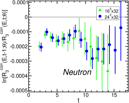
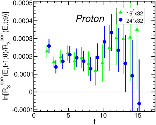
Figure 7: The same figure as Fig. 6 for clover fermion in $16^{3}\times 32$ and $24^{3}\times 32$ lattice. (top) neutron case, (bottom) proton case.

In Fig. 7 we compare the effective mass plot of $R^{\rm corr}_{3}(E,t;\theta)$ at $\theta=0.1,\,E=0.004$ in the larger volume with that in the smaller volume. It is clear that the EDM signal remains non-zero in the larger volume. Results in both volumes are consistent with each other within large errors. We can conclude that the EDM signal obtained with this method does not vanish in both volumes.

IV.3 Boundary effect of the electric field

The electric field in our method breaks periodicity in the time direction, leading to a large non-uniformity near the boundary between $t=1$ and $t=T$. Since we put a source at $t=1$, the EDM signal may be affected by the non-uniform electric field. In order to investigate how the EDM signal is affected by this boundary effect, we repeat the EDM calculation on a $24^{3}\times 32$ with the clover fermion at the heaviest quark mass, moving the source point to the different time slice but keeping other conditions fixed.

In the previous calculation at $t_{\rm src}=1$, we observed that the plateau seems to exist at $t\geq 8$. Since this indicates that the effect of boundary may be small at $t=8$, we take a new source point at $t_{\rm src}=8$. If we need a minimum plateau length of 5 for a reliable fit, we wonder be using a plateau at $t=15-19$ for $t_{\rm src}=8$. Since the time slice $t=19$ or 20 is largely separated from the boundary at $t=T=32$, the boundary effect to the plateau as a whole is expected to be small. Therefore $t_{\rm scr}=8$ is a reasonable choice.

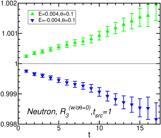
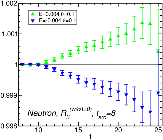
Figure 8: These figures show the time dependence of $R_{3}^{(\rm w/o\theta=0)}(E,\theta,t)$ at $\theta=0.1$ and $\kappa=0.1320$. Different figures show that source point $t_{\rm src}$ is in a different position in time direction. (top) $t_{\rm src}=1$ (bottom) $t_{\rm src}=8$.

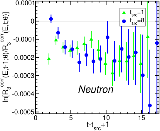
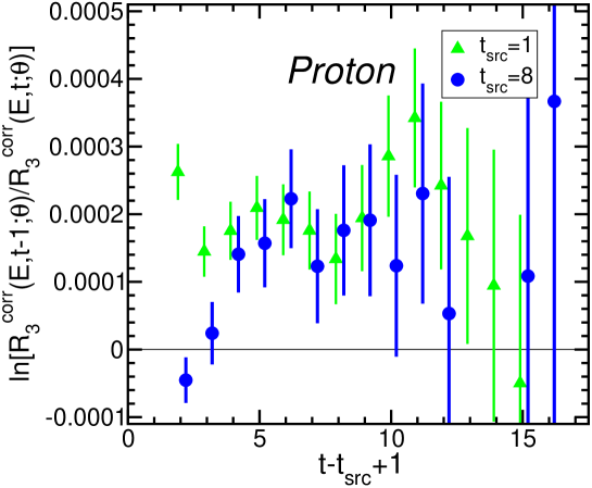
Figure 9: These figures show the effective mass plot of the spin ratio, $R^{\rm corr}_{3}(E,t;\theta)$, in both $t_{\rm src}=1$ and $t_{\rm src}=8$ at $\theta=0.1$ and $\kappa=0.1320$.

In Fig. 8 we compare the time dependence of $R_{3}^{(\rm w/o\theta=0)}(\pm E,\theta,t)$ for two different source points, $t_{\rm src}=1$ and $t_{\rm src}=8$. We clearly observe a different time dependence of $R_{3}^{(\rm w/o\theta=0)}$ for two sources at small time slices, $t-t_{\rm src}\leq 4$. We think that large deviations of $R_{3}^{(\rm w/o\theta=0)}$ from unity at $t-t_{\rm src}\leq 4$ for the $t_{\rm src}=1$ case is an effect of the large non-uniform electric field near the boundary between $t=1$ and $t=T$. On the other hand, the deviation of $R_{3}^{(\rm w/o\theta=0)}$ from unity becomes visible around $t-t_{\rm src}\simeq 4$ for the case of $t_{\rm src}=8$. Since the plateau of the nucleon effective mass appears around $t-t_{\rm src}\simeq 5-6$, contributions from excited states to $R_{3}^{(\rm w/o\theta=0)}$ become small and the nucleon state dominates around this range of $t$ in the case of $t_{\rm src}=8$. In Fig. 9 we plot the effective mass of $R_{3}^{\rm corr}(E,\theta=0,t)$ for the $t_{\rm src}=8$ case, together with that for the $t_{\rm src}=1$ case. We notice that the plateau starts around $t-t_{\rm src}=5$ for the $t_{\rm src}=8$ case. For the $t_{\rm src}=1$ case, on the other hand, the values of effective mass of $R_{3}^{\rm corr}(E,\theta=0,t)$ around $t-t_{\rm src}=4-6$ seems smaller than the plateau of the $t_{\rm src}=8$ case, suggesting that the boundary effects, observed in $R_{3}^{(\rm w/o\theta=0)}$ at small $t-t_{\rm src}$, still remain in the effective mass around $t-t_{\rm src}=4-6$. Therefore, to avoid possible contaminations from the boundary effect, we take sufficiently large separations such that $t-t_{\rm src}=8-11$ for the fit of $R_{3}^{\rm corr}(E,\theta=0,t)$ in the case of $t_{\rm src}=1$.

An important lesson here is that we should take the starting point of the fitting range as far from the source as possible, if the source is placed near the boundary such as $t_{\rm src}=1$. This caution should be applied to all other data obtained with $t_{\rm src}=1$.

Fitting with $R_{3}^{\rm corr}$ exponentially in $5\leq t-t_{\rm src}\leq 9$ with $t_{\rm src}=8$, we obtain

$$d_{N}=\left\{\begin{array}[]{rc}-0.025(8)\,e\cdot\rm{fm}&\textrm{(Neutron)}\\ 0.024(11)\,e\cdot\rm{fm}&\textrm{(Proton)}\\ \end{array}\right.,$$ (28)

while for the $t_{\rm src}=1$ case we have

$$d_{N}=\left\{\begin{array}[]{rc}-0.030(8)\,e\cdot\rm{fm}&\textrm{(Neutron)}\\ 0.036(11)\,e\cdot\rm{fm}&\textrm{(Proton)}\\ \end{array}\right.$$ (29)

with $t-t_{\rm src}\in[7,11]$ as the fitting range. Two results are consistent with each other within large statistical errors. Similarly, on a $16^{3}\times 32$ lattice, we obtain

$$d_{N}=\left\{\begin{array}[]{rc}-0.021(11)\,e\cdot\rm{fm}&\textrm{(Neutron)}\\ 0.026(13)\,e\cdot\rm{fm}&\textrm{(Proton)}\\ \end{array}\right.$$ (30)

for the clover fermion and

$$d_{N}=\left\{\begin{array}[]{rc}-0.017(8)\,e\cdot\rm{fm}&\textrm{(Neutron)}\\ 0.020(10)\,e\cdot\rm{fm}&\textrm{(Proton)}\\ \end{array}\right.$$ (31)

for the domain-wall fermion. The fitting range is $t-t_{\rm src}\in[6,11]$ with $t_{\rm src}=1$ for both fermions. These values, summarized in Table 2, have the same sign and a similar order of magnitude to the EDM form factor previously obtained on a $16^{3}\times 32$ lattice with the domain-wall fermion with the form factor method, which is given by $F_{3}(q^{2}\simeq 0.58{\rm GeV}^{2})/m_{N}=-0.024(5)$ e$\cdot$fm for neutron and $0.021(6)$ e$\cdot$fm for protonShitani_form . These agreements of sign and magnitude between the two methods support that the viability of this method explored in this paper.

IV.4 $E$ and $\theta$ dependence

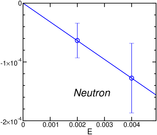
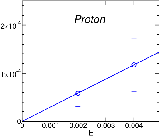
Figure 10: The $E$ dependence for the fitting results of $R^{\rm corr}_{3}(E,t;\theta)$ in the range of $[7,12]$ at $\theta=0.1$ with domain-wall fermion (top) for neutron, (bottom) for proton. The solid line denotes a result of linear fit.

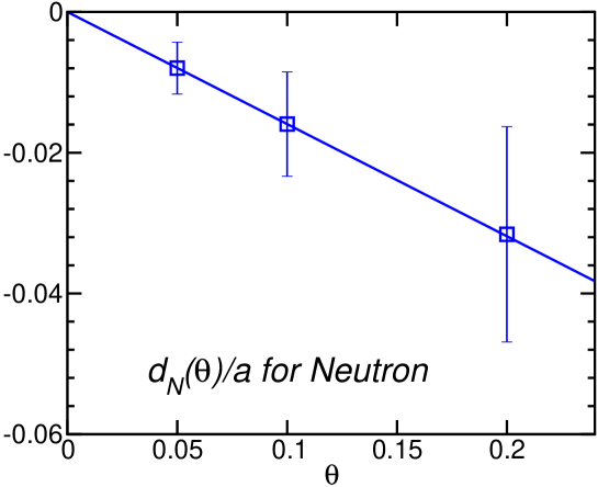
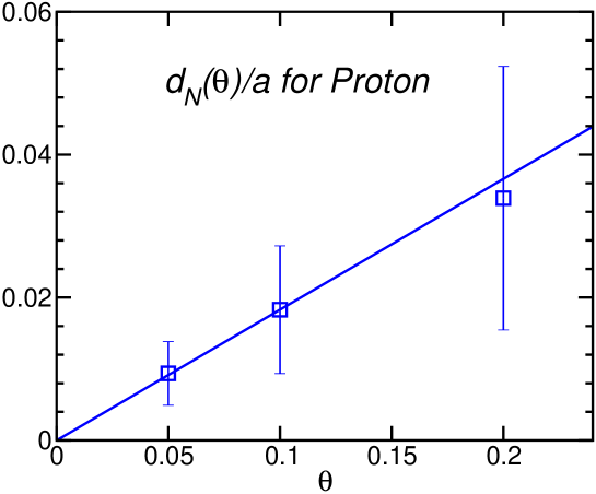
Figure 11: The $\theta$ dependence for the fitting results of $R^{\rm corr}_{3}(E,t;\theta)$ in the range of $t\in[7,12]$ at $E=0.004$ with domain-wall fermion (top) for neutron, (bottom) for proton. The solid line denotes a result of linear fit.

In Fig. 10 we plot values of EDM as a function of $E$ for neutron(upper) and proton (lower) at $\theta=0.1$. Observing the expected linear dependence on $E$ for both cases, we conclude that $O(E^{3})$ contributions in (8) are negligible. Fig. 11 shows $d_{N}(\theta)$ in lattice unit as a function of $\theta$ at $E=0.004$, assuming the linear $E$ dependence of the fitted EDM signal. We again confirm that the linearity in $\theta$ is good and thus $O(\theta^{3})$ contributions in (9) are reasonably small.

We concluded that our choices of $(E,\theta)=(0.004,0.1)$ are small enough to ensure linear dependences of the EDM signal on both $E$ and $\theta$, which we assume in the analysis in the rest of this paper.

IV.5 Average over the electric field

Averaging over three directions of the electric field is not so useful in quenched simulation. This way of increasing statistics, however, may become important in full QCD case since the number of full QCD configurations is limited. In this subsection we investigate the effectiveness of this method and the related question of the independence of the EDM signal on the direction of the electric field.

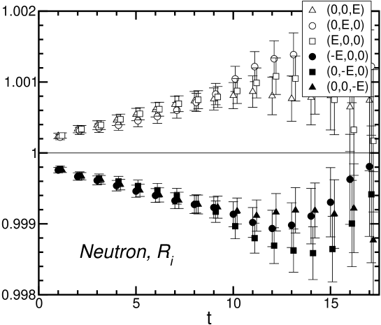
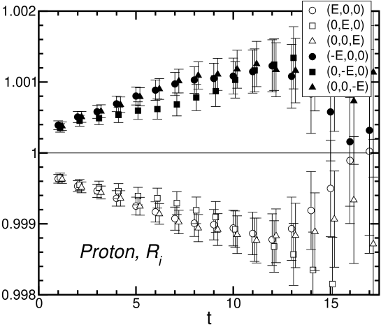
Figure 12: The time dependence of $R_{i}(E,\theta,t)$ for three direction of electric field, which is $(E,0,0),\,(0,E,0),\,(0,0,E)$. The difference with open and filled symbol denote the different sign of electric field. (top) neutron case, (bottom) proton case.

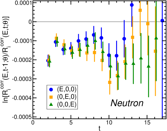
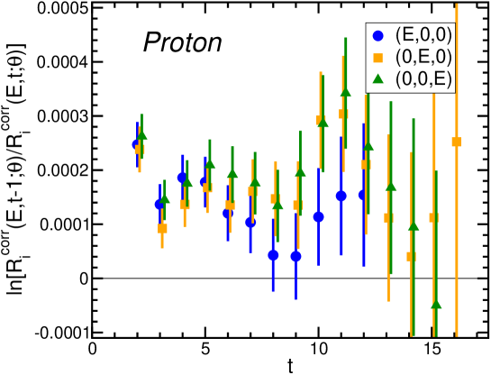
Figure 13: The effective mass plot of $R^{\rm corr}_{i}(E,\theta,t)$ of each directions of electric field. (top) neutron case, (bottom) proton case.

Using eq. (18), eq. (II.2) and eq. (II.2) for $\vec{E}=(0,0,E)$, $(E,0,0)$, and $(0,E,0)$, we obtain $R_{i}$ as a function of $E$ for each $\vec{E}$ on a $24^{3}\times 32$ lattice with the clover fermion at heaviest quark mass. In Fig. 12, $R_{i}$ shows similar time dependences for all $i$ . EDM signals, given in Fig. 13, are also comparable in the similar time range among different directions. We confirm the consistency among extraction of the EDM signal from three different directions using the formulae in eqs. (18)-(II.2).

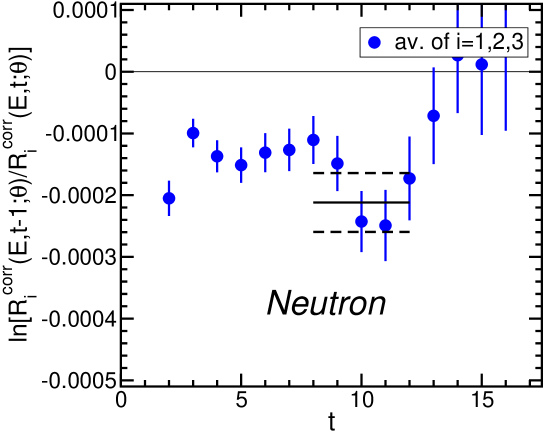
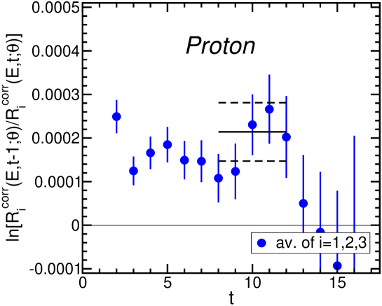
Figure 14: These figures show the effective mass plot of the average of $R^{\rm corr}_{i}(E,\theta,t)$ for three directions of electric field with $\kappa=0.1320$. (top) neutron case, (bottom) proton case.

We now consider the average over 3 directions. In Fig. 14 the effective mass of the average, $R^{\rm corr}(E,\theta,t)\equiv\sum_{i}R_{i}^{\rm corr}(E,\theta,t)$ is plotted as a function of $t$. Fitting it exponentially at $7\leq t-t_{\rm src}\leq 11$, we obtain

$$d_{N}=\left\{\begin{array}[]{rc}-0.0276(72)\,e\cdot\rm{fm}&\textrm{(Neutron)}\\ 0.0278(87)\,e\cdot\rm{fm}&\textrm{(Proton)}\end{array}\right..$$ (32)

Although errors are reduced in the effective mass, the reduction in $d_{N}$ is much smaller than $1/\sqrt{3}$. We conclude that the error reduction by this averaging is limited, due to the possible correlation among $R_{i=1,2,3}(E,\theta,t)$,

V Quark Mass Dependence

In this section we study the quark mass dependence of EDM using the clover fermion on a $24^{3}\times 32$ lattice.

V.1 Quenched effects

It is well known in full QCD that EDM generated by the $\theta$ term must vanish in the chiral limit. This can be seen from the fact that the CP-violation Lagrangian after an appropriate chiral rotation Crewther ,

$$\delta\mathcal{L}_{\rm CP}=i\theta\bar{m}\sum_{i=u,d,s}\bar{\psi}_{i}\gamma_{5}\psi_{i}(x),\quad\bar{m}=\Big{(}\sum_{i=u,d,s}m_{i}^{-1}\Big{)}^{-1},$$ (33)

vanishes in the massless limit of any quarks. (See RBC for more detailed argument on this property.)

In quenched QCD, however, this argument fails since the $\theta$ parameter can not be translated to the above form in the absence of the chiral anomaly, which requires the quark determinant. Therefore CP-violating observables generated by the $\theta$ term may remain non-zero in the zero quark mass limit. Indeed, as discussed in RBC , zero modes of the quark Dirac operator can generate CP-odd contributions even in the massless limit. It is not so easy, however, to determine the explicit quark mass dependence of the EDM from the general argument in quenched QCD.

Recently, from the numerical simulation of the instanton liquid model Faccioli , the $1/m_{q}^{2}$ dependence for NEDM has been reported near the chiral limit of quenched QCD. The partially quenched chiral perturbation theory Connell , on the other hand, has suggested the $1/m_{\pi}^{3}$ behavior in the finite volume of $L^{3}$ at fixed sea quark mass $m_{\rm sea}$ such that

$$d_{N}^{\rm P.Q.ChPT}\sim-\frac{e\theta m_{\rm sea}}{m_{\pi}^{3}L^{3}}f_{\pi},$$ (34)

from the leading contribution of one-loop graphs.

V.2 Quark mass dependence of EDM

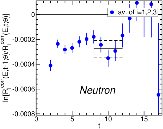
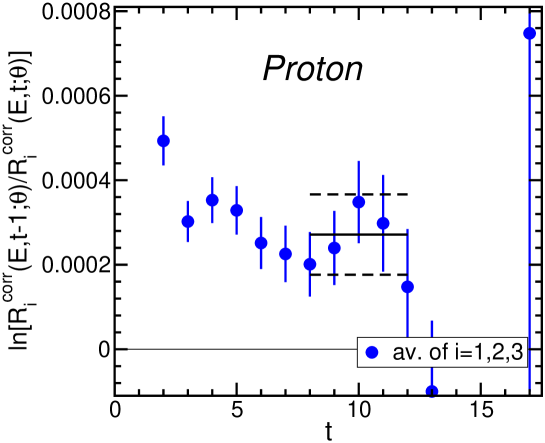
Figure 15: The same figure as Fig. 14 with $\kappa=0.1330$. (top) neutron case, (bottom) proton case.

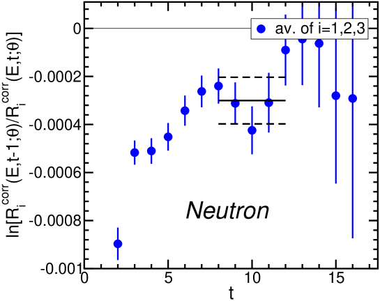
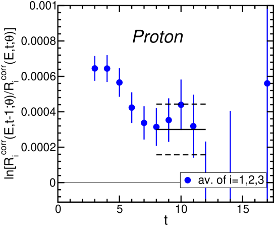
Figure 16: The same figure as Fig. 14 with $\kappa=0.1340$. (top) neutron case, (bottom) proton case.

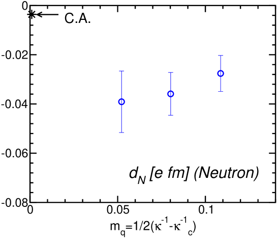
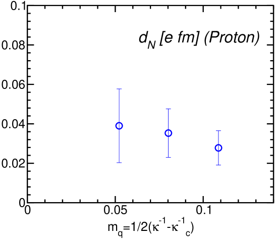
Figure 17: The mass dependence of EDM factor with clover fermion. In top figure the star symbol shows the prediction from current algebra in Crewther . (top) neutron case, (bottom) proton case.

We calculate EDM at three different quark masses with the clover fermion on a $24^{3}\times 32$ lattice. In Fig. 15 and Fig. 16 we plot the effective mass of $R^{\rm corr}(E,\theta,t)=\sum_{i=1}^{3}R^{\rm corr}_{i}(E,\theta,t)$ as a function of $t$ at two lighter quark mass with $t_{\rm src}=1$. Signals become a little noisier and less stable as the quark mass decreases. Fitting data at $t-t_{\rm src}\in[7,10]$ for the three quark masses, we obtain the quark mass dependence of EDM for neutron and proton as shown in Fig. 17 and Table 3. Compared with the current algebra result, $-0.0036$ e$\cdot$fm Crewther ; Vecchia also shown in the top of Fig. 17, our quenched NEDM are about 10 times larger. Moreover our results suggest that EDM does not vanish in the chiral limit for both neutron and proton. We consider that the larger value of NEDM we focus is partly due to the quenched effect. Because of large statistical errors, we can not distinguish the functional form of the mass dependence of EDM, whether it stays constant or diverges in the chiral limit.

V.3 Quark mass dependence of the CP-odd phase factor

In addition to the EDM, using the clover fermion, we calculate a simpler quantity $f_{N}^{1}$, the CP-odd phase factor of the nucleon propagator, defined in Ref.Shitani_form as

$$\langle N(\vec{p},t)\bar{N}(\vec{p},0)Q\rangle=|Z_{N}|^{2}e^{-E_{N}t}\frac{f_{N}^{1}m_{N}}{2E_{N}}\gamma_{5}.$$ (35)

Since the CP-odd phase factor arises from CP-violation effects of the $\theta$ term, $f_{N}^{1}$ would vanish in the chiral limit of full QCD. In quenched QCD, however, this quantity also may remain non-zero in chiral limit because of the same reason as the EDM.

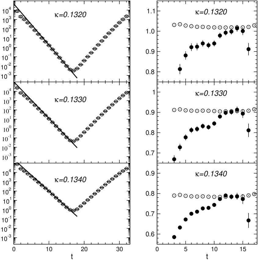
Figure 18: In the left figure we show that the time dependence of nucleon propagator in next leading order of $\theta$ at each quark mass: $-{\rm tr}\langle NNQ\rangle\frac{\gamma_{5}}{2}$. The straight line represents fitting function with $f(x)=Ae^{-m_{N}t}$. In right figure we show that the comparison with exponent of nucleon propagator between the leading(open circles) and the next to leading order(solid circles).

In Fig. 18, we show the time dependence of the nucleon propagator at the next leading in $\theta$, $-{\rm tr}[\langle N(\vec{0},t)\bar{N}(\vec{0},0)Q\rangle\frac{\gamma_{5}}{2}]$ (left), and effective masses of the leading nucleon propagator in $\theta$, ${\rm tr}[\langle N(\vec{0},t)\bar{N}(\vec{0},0)\rangle\frac{1+\gamma_{4}}{2}]$, as well as the next leading one (right) at 3 quark masses. Since effective mass plots show the agreement of masses between two propagators around $t=10$, we extract $f_{N}^{1}$ by fitting ${\rm tr}[\langle N(\vec{0},t)\bar{N}(\vec{0},0)Q\rangle\frac{\gamma_{5}}{2}]$ at $9\leq t\leq 12$ in the form of (35), where $|Z_{N}|^{2}$ and $m_{N}$ have been fixed from the leading propagator.

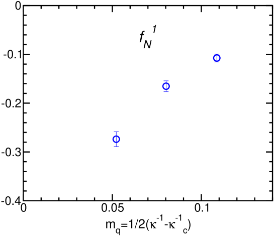
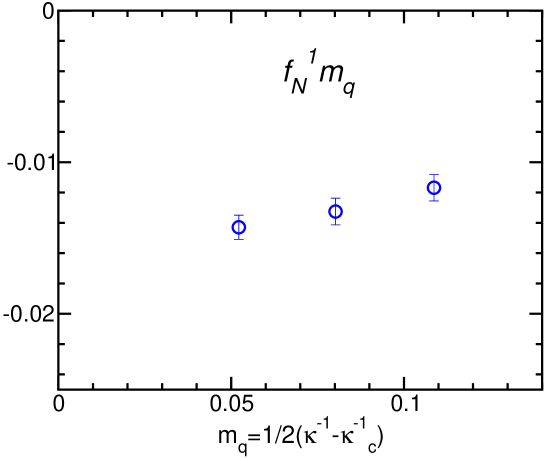
Figure 19: The mass dependence of CP-odd phase factor with clover fermion. The top figure presents $f_{N}^{1}$ at each quark mass, and the bottom figure presents the $f_{N}^{1}$ multiplied by quark mass.

The quark mass dependence of $f_{N}^{1}$ is given in Fig. 19 and Table 3. It is noted that errors of $f_{N}^{1}$ are much smaller than those of EDM. The top of Fig. 19 shows that $f_{N}^{1}$ does not vanish in chiral limit and moreover it seems to diverge as $1/m_{q}$ in this limit. To see this behavior more clearly, we plot $f_{N}^{1}$ multiplied by the quark mass $m_{q}=(\kappa^{-1}-\kappa_{c}^{-1})/2$ as a function of $m_{q}$ in the bottom of Fig. 19. The fact that $f_{N}^{1}m_{q}$ seems almost constant at this range of the quark mass suggests that $f_{N}^{1}$ may diverge as $1/m_{q}$ in the chiral limit. It may be interesting to confirm this behavior of $f_{N}^{1}$ by some theoretical considerations.

VI Summary and Discussion

In this paper, we have investigated the viability of an old idea for calculating the nucleon EDM by introducing a uniform and static electric field. In this setup the nucleon EDM appears directly in the energy difference between spin-up and spin-down states of the nucleon. To introduce the complex $\theta$ term into lattice QCD calculations, we used the reweighting technique with the factor $e^{i\theta Q}$. We have demonstrated that this reweighting method indeed works as long as $\theta$ is small enough, by calculating the nucleon EDM in quenched QCD on a $16^{3}\times 32$ lattice at a relatively heavy quark mass. We found that the quality of signals is not very sensitive to lattice fermion formulations employed, domain-wall fermion and clover fermion in our study. Using the clover fermion on a $24^{3}\times 32$ lattice, we investigated the effect of non-uniformity of our electric field induced at the boundary in time direction. Even if the source point of nucleon is placed near the boundary, the effect to the nucleon EDM disappears for large enough $t$, while the effect becomes smaller even at small $t$ if the source is placed away from the boundary. We also found that the finite size effect to EDM is not so large: results between (1.6 fm)³ and (2.4 fm)³ boxes agree within errors.

We investigated the quark mass dependence of the nucleon EDM and the CP-odd phase factor $f_{N}^{1}$ in quenched approximation on a larger volume with the clover fermion. Both quantities do not seem to vanish in the chiral limit, in contrast to full QCD where effects of the $\theta$ term disappear for a massless quark. Therefore non-vanishing behaviors of EDM and $f_{N}^{1}$ are purely quenching effects. In particular, $f_{N}^{1}$ seems to diverge as $\mathcal{O}(1/m_{q})$ in chiral limit. It is, however, difficult to determine precise quark mass dependences of these quantities in quenched QCD, due to larger statistical errors.

This work shows that the external electric field method is simple and straightforward for the determination of the EDM in lattice QCD. In particular, the success with clover fermion in this method is significant for applications to full QCD simulations. We are currently carrying out the EDM calculation using $N_{f}=2$ dynamical clover configurations generated by the CP-PACS collaborationShintani_wE2 .

Appendix A Electric polarizability of Neutron

In this appendix we discuss the electric polarizability of the neutron. This observable can also be obtained by the external field method employed in our calculation, as has been done in refs. Fiebig ; Christensen . We compare our results with theirs.

A.1 Definition

The electric polarizability $\alpha_{N}$ is defined as the coefficient of the $\vec{E}^{2}$ term in the expansion of the $\vec{E}$ dependent nucleon mass $m_{N}(\vec{E})$:

$$\Delta m_{N}(\vec{E})=m_{N}(\vec{E})-m_{N}(0)=-\frac{1}{2}(4\pi\alpha_{N})(e^{-1}a^{-2}\vec{E})^{2}.$$ (36)

which is measured by Compton scattering experiments. Note that the electric field $\vec{E}$ here is dimensionless. A recent Compton scattering experiment gives

$$\alpha^{\rm exp}_{N}=(1.16\pm 0.15)\times 10^{-3}\,\textrm{fm}^{3}$$ (37)

for the neutronPDG . In the lattice calculation the effective mass shift is calculated by

$$r_{N}(\vec{E},t) = \frac{\langle N\bar{N}\rangle(\vec{E},t)}{\langle N\bar{N}\rangle(\vec{0},t)},$$ (38)

$$\Delta m_{N}(\vec{E}) = \ln\left[\frac{r_{N}(\vec{E},t)}{r_{N}(\vec{E},t+1)}\right].$$ (39)

where $\langle N\bar{N}\rangle(\vec{E},t)$ denotes the nucleon propagator in the presence of the constant electric field $\vec{E}$ without reweighting $e^{i\theta Q}$. In order to remove spurious contributions odd in $\vec{E}$ from the effective mass shift, we take an average over $\vec{E}$ and $-\vec{E}$, by replacing

$$r_{N}(\vec{E}) \rightarrow \frac{1}{2}({r_{N}(\vec{E},t)}+{r_{N}(-\vec{E},t)})$$ (40)

in eq.(39).

A.2 Numerical results on a $16^{3}\times 32$ lattice

Our lattice setup for the calculation of the electric polarizability is same as the one employed for the NEDM calculation in sec. IV.1. In particular, the real electric field $\vec{E}=(0,0,E)$ in Minkovski space is introduced by the replacement of eq. (12). Although the periodicity in time direction is broken by this electric field, the boundary conditions for the fermion are periodic in both time and spatial directions on a $16^{3}\times 32$ lattice. We employ the domain-wall fermion at $E=4\times 10^{-3}$ and $E=2\times 10^{-3}$. As a comparison we also employ the clover fermion at $E=4\times 10^{-3}$.

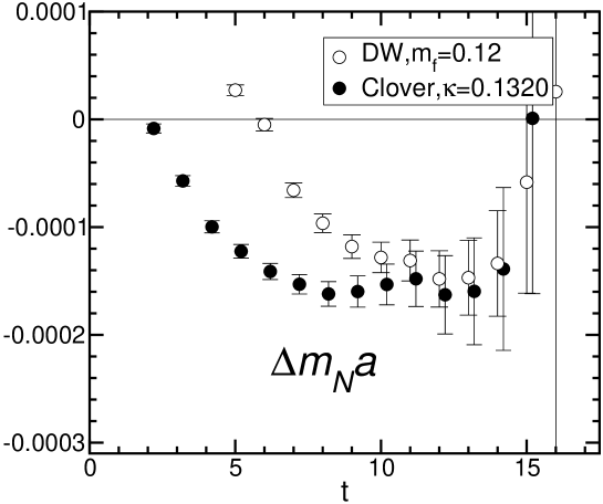
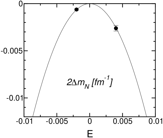
Figure 20: (Top) The effective mass shift plot as Fig. 25 in periodic boundary condition with domain-wall and clover fermion at $E=4.0\times 10^{-3}$. (Bottom) The $E$ dependence of the mass shift of the above results from exponentially fitting $r_{N}$ in the range of $[9,14]$ with domain-wall fermion. The solid line presents fit results with the function $f(E)=\alpha E^{2}$.

In the top of Fig. 20 we show the effective mass plot of $r_{N}$ in eq. (39) for domain-wall and clover fermions on same configurations. We observe the plateau starting around $t=7$ for the clover fermion and around $t=10$ for the domain-wall fermion. From the exponential fit of $r_{N}(t)$ at $9\leq t\leq 14$, we obtain $\Delta m_{N}$, whose values are given in Table 4.

In the bottom of Fig. 20 we present the $E$ dependence of the mass shift $2\Delta m_{N}$ for the domain-wall fermion. By fitting data with $-4\pi\alpha_{N}(e^{2}a^{4})^{-1}E^{2}$, we obtain the electric polarizability for neutron :

$$\alpha_{N}=1.32(2)\times 10^{-4}\,\textrm{fm}^{3}$$ (41)

in the unit of $e^{2}(4\pi)^{-1}a^{3}\simeq 0.73\times 10^{-5}$ fm³ with the fine-structure constant $\alpha=e^{2}/(4\pi)=1/137$.

This value, obtained in quenched QCD at $a\simeq 0.1$ fm and $m_{PS}/m_{V}\simeq 0.88$. is $1/10$ times smaller than the experimental value $\alpha_{N}^{\rm exp}=1.16(15)\times 10^{-3}$ fm³, but the sign of $\alpha_{N}$ agrees.

A.3 Results on $24^{3}\times 32$ with two different source points

We also calculate the electric polarizability of the neutron on a larger volume, $24^{3}\times 32$, using the clover fermion at $\kappa=0.1320$. As in sec. IV.3, we employ two different source points, $t_{\rm src}=1$ and $t_{\rm src}=8$, to investigate the effect of the gap in $E$ at the boundary to the electric polarizability.

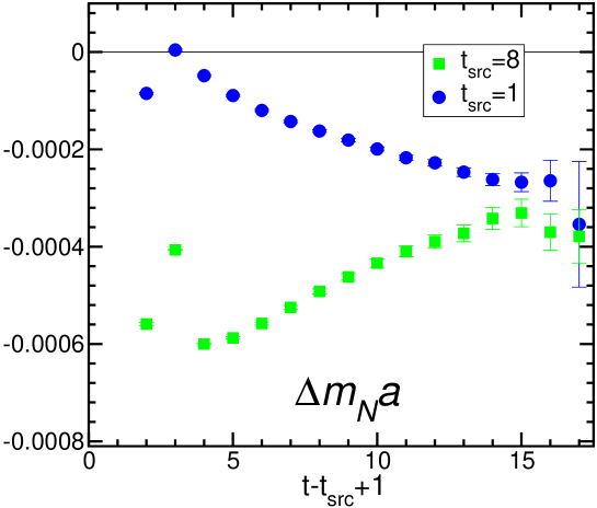
Figure 21: This figure shows the comparison with different source point $t_{\rm src}$. We plot the effective mass shift as Fig. 25 in periodic boundary condition with clover fermion at $\kappa=0.1320$ and $E=4.0\times 10^{-3}$ in large lattice size $24^{3}\times 32$.

In Fig. 21 we present the effective mass shift, $\Delta m_{N}a$, for both $t_{\rm src}=1$ and $t_{\rm src}=8$. Compared with results on the smaller volume in sec. A.2, plateaus seem to appear at very large $t$ for both sources or even $\Delta m_{N}a$ may not reach the plateau at $t\leq 16$. Even though an identification of plateaus is less reliable on the larger volume, we fit data exponentially in $t$ at $13\leq t\leq 16$ and give values of $\Delta m_{N}a$ in Table 4. As seen in the table, the magnitude of fitted values is larger than the value on the smaller volume. We think that this discrepancy is mainly caused by contaminations from excited states on the larger volume. We need larger time separations to extract the ground state contribution unambiguously. We also observe large differences in the effective mass at small $t$ between $t_{\rm src}=1$ and $t_{\rm src}=8$. This indicates that the electric polarizability is quite sensitive to the boundary effect.

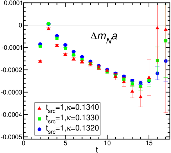
Figure 22: We plot the effective mass shift as Fig. 21 with several quark masses.

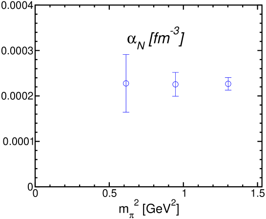
Figure 23: This figure shows the mass dependence of electric polarizability of neutron with same parameter as Fig. 22.

In Fig. 22 we plot the effective mass shift at different quark mass after taken average over three directions of electric field with $t_{\rm src}=1$ on $24^{3}\times 32$. We observe that the time behavior is not so different with each other, and therefore its value will not depend on the quark mass strongly. Fig. 23 and Table 5 shows the converted results to electric polarizability using fitting data of $\Delta m_{N}$ in each $\kappa$. In these heavier masses, the results seems to be constant for square of pion mass, though statistic errors are still large. Therefore more statistics are probably needed to give a precise value of the neutron electric polarizability in the chiral limit.

A.4 Comparison with previous calculations

As a test of our method, we use same lattice parameters as in previous calculationsFiebig ; Christensen : Accumulating 40 quenched configurations generated by the plaquette action at $\beta=6.0$ ( $a\simeq 0.1$ fm ) on a $24^{4}$ lattice, we calculate the electric polarizability by the Wilson fermion action at $\kappa=0.1515$, which is the heaviest quark mass in Christensen . With the periodic boundary condition in spatial directions but the Dirichlet boundary condition in the time direction, the nucleon propagator is calculated for a point source at $t=1$ and a point sink at $t$.

The electric field is introduced into all spatial link variables in the expanded form:

$$U_{3}(x)\longrightarrow e^{iqEt}U_{3}(x)\simeq(1+iqEt)U_{3}(x),$$ (42)

where we use an electric field in Euclidean space, which corresponds to the imaginary value in Minkovski space. Therefore the $E$ dependence of the mass shift $\Delta m_{N}$ is given by

$$\Delta m_{N}(i\vec{E})=-\frac{1}{2}(4\pi\alpha_{N})(ie^{-1}a^{-2}\vec{E})^{2}=\frac{1}{2}(4\pi\alpha_{N})e^{-2}a^{-4}\vec{E}^{2}$$ (43)

with the electric polarizability $\alpha_{N}$. As in Christensen , we employ $E=\pm 1.08\times 10^{-3},\,\pm 4.32\times 10^{-3},\,\pm 8.64\times 10^{-3}$ in the actual calculation. Note that the periodicity of spatial link variables in the time direction is explicitly violated partly due to the fact that $E\not=2\pi/L$ and partly due to the expansion (42).

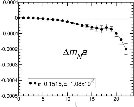
Figure 24: The effective mass shift plot for neutron with Wilson fermion at $E=1.08\times 10^{-3}$ and $\kappa=0.1515$, The initial time of our data is set up to be same as Christensen .

Fig. 24 shows the effective mass shift for neutron in eq. (39) at $|E|=1.08\times 10^{-3}$. Our data in Fig. 24 roughly agree with filled circle symbols in Fig. 6 of Christensen . Unfortunately a candidate for a possible plateau appears only at $15\leq t\leq 19$. Assuming that this is indeed a real plateau, we fit $\Delta m_{N}$ exponentially in $t$ at $15\leq t\leq 19$ and gives values at each $E$ in Table 4.

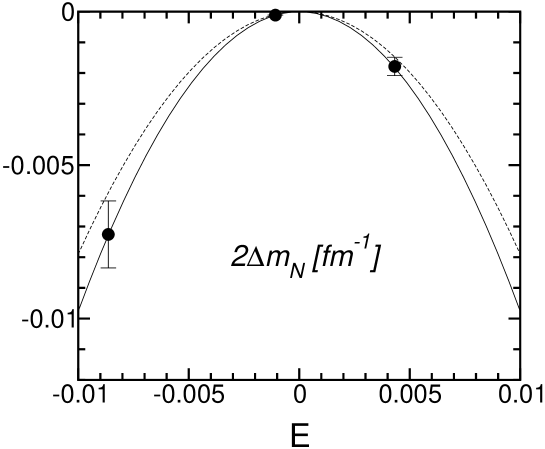
Figure 25: This figure presents the $E$ dependence of the mass shift. The solid line denotes fitting results with our data and the broken line denotes results in Christensen . Each our data are given by fitting in the time range of $[15,19]$.

In Fig. 25 we plot the $E$ dependence of mass shift $\Delta m_{N}$. By fitting data with $\frac{1}{2}(4\pi\alpha_{N})e^{-2}a^{-3}E^{2}$, we obtain a coefficient $\alpha_{N}$, the value of electric polarizability:

$$[\alpha_{N}]_{\rm Dirichlet}=-8.5(8)\times 10^{-4}\,\textrm{fm}^{3}.$$ (44)

This value agree with the value in Christensen , $[\alpha_{N}]_{\rm Dirichlet}=-7.9(5)\times 10^{-4}$ fm³, within about one-sigma error. Surprisingly the sign of this result is opposite to the result (41) obtained by the real electric field in Minkovski space and to the experimental value in eq. (37). In addition we confirm that the negative value of $\alpha_{N}$ is obtained even if we use the real electric field in Minkovski space in the Dirichlet boundary condition. Therefore the wrong sign of $\alpha_{N}$ in this case is not caused by the way of introducing the electric field (Euclid or Minkovski) but is related to the boundary condition in the time direction. We think that $T=24$ is too short to suppress contributions from excited states to $\alpha_{N}$. In order to obtain a reliable estimate for $\alpha_{N}$, one should investigate dependences of results on the lattice set-up such as the boundary conditions, the source point or the way of introducing the electric field. We leave these studies in future investigations.

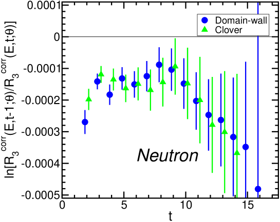
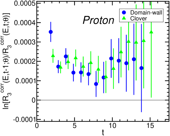
Figure 6: The effective mass plot of $R^{\rm corr}_{3}(E,t;\theta)$ in $E=0.004,\,\theta=0.1$ with domain-wall and clover fermions in $16^{3}\times 32$ lattice. (top) neutron case, (bottom) proton case.

Table 1: Table for lattice parameters. The column of $(A,B)$ denotes the smearing source parameter in the exponent

Fermion	$\beta$	$L^{3}\times T\times N_{s}$	$M$	$a^{-1}\,[\textrm{GeV}]$	$m_{q}$	$(A,B)$	$m_{PS}/m_{V}$	$m_{N}a$
Domain-wall	$2.6$	$16^{3}\times 32\times 16$	$1.8$	$1.902(50)$	$0.12$	(1.28,0.40)	$0.8781(4)$	$1.1130(15)$
Fermion	$\beta$	$L^{3}\times T$	$c_{SW}$	$a^{-1}\,[\textrm{GeV}]$	$\kappa$	$(A,B)$	$m_{PS}/m_{V}$	$m_{N}a$
Clover	$2.6$	$16^{3}\times 32$	$1.340$	$1.902(50)$	$0.1320$	(1.55,0.24)	$0.8508(5)$	$1.0202(17)$
Clover	$2.6$	$24^{3}\times 32$	$1.340$	$1.902(50)$	$0.1320$	(1.55,0.35)	$0.8494(1)$	$1.0186(9)$
					$0.1330$	(1.55,0.31)	$0.8026(2)$	$0.9058(14)$
					$0.1340$	(1.55,0.27)	$0.7253(2)$	$0.7843(16)$
					$\kappa_{c}=0.1359(1)$

Table 2: Table for EDM results in some lattice parameters

fermion	$m_{N}a$	lattice size	source point	fitting range	$d_{N}$ (Neutron)	$d_{N}$ (Proton)
domain-wall	$1.1130(15)$	$16^{3}\times 32$	$t_{\rm src}=1$	$t-t_{\rm src}\in[6,11]$	$-0.0170(79)$	$0.0196(95)$
clover	$1.0202(17)$	$16^{3}\times 32$	$t_{\rm src}=1$	$t-t_{\rm src}\in[6,11]$	$-0.0205(104)$	$0.0256(125)$
clover	$1.0186(9)$	$24^{3}\times 32$	$t_{\rm src}=1$	$t-t_{\rm src}\in[7,11]$	$-0.0304(78)$	$0.0361(111)$
clover	$1.0200(9)$	$24^{3}\times 32$	$t_{\rm src}=8$	$t-t_{\rm src}\in[5,9]$	$-0.0246(83)$	$0.0237(112)$

Table 3: The mass dependence of EDM factor from exponential fit in the range $8\leq t\leq 12$ for $R^{\rm corr}(E,\theta,t)$ which is the average over indices $i=1,2,3$ and CP-odd phase factor in the next leading term of nucleon propagator.

	Neutron			Proton		$f_{N}^{1}$	$f_{N}^{1}m_{q}$
$\kappa$	fit	$d_{N}\,[\textrm{e}\cdot\textrm{fm}]$		fit	$d_{N}\,[\textrm{e}\cdot\textrm{fm}]$
0.1320	$-0.000212(48)$	$-0.0276(72)$		$0.000214(67)$	$0.0278(87)$	$-0.1075(80)$	$-0.0117(8)$
0.1330	$-0.000276(67)$	$-0.0359(87)$		$0.000271(95)$	$0.0353(123)$	$-0.1653(111)$	$-0.0133(9)$
0.1340	$-0.000300(97)$	$-0.0391(125)$		$0.000300(143)$	$0.0390(187)$	$-0.2738(152)$	$-0.0143(8)$

Table 4: Summary of the fitting results of mass shift of neutron with different boundary condition and fermions.

gauge action	mass	lattice size	B.C.	$t_{\rm src}$	$E$	$\Delta m_{N}a$
Domain-wall fermion
RG Iwasaki $\beta=2.6$	$m_{f}=0.12$	$16^{3}\times 32$	Periodic	$t_{\rm src}=1$	Real, 0.002	$-$0.0000375(44)
					Real, 0.004	$-$0.000157(18)
Clover fermion
RG Iwasaki $\beta=2.6$	$\kappa=0.1320$	$16^{3}\times 32$	Periodic	$t_{\rm src}=1$	Real, 0.004	$-$0.000155(20)
		$24^{3}\times 32$	Periodic	$t_{\rm src}=1$	Real, 0.004	$-$0.000265(22)
				$t_{\rm src}=8$	Real, 0.004	$-$0.000356(50)
Wilson fermion
Plaquette $\beta=6.0$	$\kappa=0.1515$	$24^{3}\times 24$	Dirichlet	$t_{\rm src}=1$	Imag, 0.00108	$-$0.000069(2)
					Imag, 0.00432	$-$0.00107(18)
					Imag, 0.00864	$-$0.00435(65)

Table 5: Summary of the fitting results of polarizability of neutron with clover fermion action at three different quark masses after average over three directions of electric field.

gauge action	lattice size	B.C.	mass	$t_{\rm src}$	$E$	$\alpha_{N}\,({\rm fm}^{-3})$
RG Iwasaki $\beta=2.6$	$24^{3}\times 32$	Periodic	$\kappa=0.1320$	$t_{\rm src}=1$	Real, 0.004	0.000227(14)
			$\kappa=0.1330$	$t_{\rm src}=1$	Real, 0.004	0.000226(26)
			$\kappa=0.1340$	$t_{\rm src}=1$	Real, 0.004	0.000228(63)

References

- (1) M. Kobayashi and T. Masukawa, Prog. Theor. Phys. 49, 652 (1973).
- (2) P. G. Harris et al., Phys. Rev. Lett. 82, 904 (1999), The EDM Collaboration, LANSCE Neutron EDM Experiment, http://p25ext.lanl.gov/edm/edm.html
- (3) V. F. Dmitriev and R. A. Sen’kov, Phys. Rev. Lett. 91, 212303 (2003)
- (4) M. V. Romalis, W. C. Griffith, J. P. Jacobs and E. N. Fortson, Phys. Rev. Lett. 86, 2505 (2001).
- (5) K. Hagiwara et al., Phys. Rev. D66, 010001 (2002).
- (6) R. D. Peccei and H. R. Quinn, Phys. Rev. Lett. 38, 1440 (1977); R. D. Peccei, Adv. Ser. Direct. High Energy Phys. 3, 503-551 (1989).
- (7) R. J. Crewther, P. Di Vecchia, G. Veneziano and E. Witten, Phys. Lett. B88, 123 (1979); erratum, ibid. B91, 487 (1980).
- (8) P. Di Vecchia, Acta Phys. Austriaca Suppl. 22, 477 (1980).
- (9) S. Aoki and T. Hatsuda, Phys. Rev. D45, 2427 (1992).
- (10) H. Y. Cheng, Phys. Rev. D44, 166 (1991).
- (11) A. Pich and E. de Rafael, Nucl. Phys. B367, 313 (1991).
- (12) M. Pospelov and A. Ritz, Nucl. Phys. B558, 243 (1999); Nucl. Phys. B573, 177 (2000); Phys. Rev. Lett. 83, 2526 (1999); Phys. Rev. D63, 073015 (2001).
- (13) Chuan-Tsung Chan, E. M. Henley and T. Meissner, hep-ph/9905317.
- (14) M. Pospelov and A. Ritz, Ann. Phys. 318, 119 (2005)
- (15) S. Aoki, A. Gocksch, Phys. Rev. Lett. 63, 1125 (1989); erratum, ibid. 65, 1172 (1990).
- (16) S. Aoki, A. Gocksch, A. V. Manohar, S. R. Sharpe, Phys. Rev. Lett. 65, 1092 (1990).
- (17) E. Shintani, et al., Phys. Rev. D72, 014504 (2005).
- (18) E. Shintani et al., PoS LAT2005, 128 (2006), hep-lat/0509123.
- (19) E. Shintani et al., PoS LAT2006, 123 (2006), hep-lat/0610022.
- (20) F. Berruto, T. Blum, K. Orginos, A. Soni, Nucl. Phys. Proc. Suppl. 140, 411 (2005); T. Blum, PoS LAT2005, 010 (2005); F. Berruto, T. Blum, K. Orginos, A. Soni, Phys. Rev. D73, 054509 (2006).
- (21) S, Aoki, in private note.
- (22) M. Okamoto, et al., (CP-PACS collaboration), Phys. Rev. D60, 094510 (1999).
- (23) A. Ali Khan, et al., (CP-PACS Collaboration), Phys. Rev. D65, 054505 (2002); erratum ibid. D67, 059901 (2003).
- (24) T. Ishikawa, et al., (CP-PACS/JLQCD Collaborations), Nucl. Phys. B (Proc. Suppl.) 140, 225 (2005), hep-lat/0409124.
- (25) Y. Kuramashi, et al., (PACS-CS Collaborations), PoS LAT2006, 029 (2006), hep-lat/0610063.
- (26) P. Weisz, Nucl. Phys. B212, 1 (1983); P. Weisz, R. Wohlert, Nucl. Phys. B236, 397 (1984); erratum, ibid. B247, 544 (1984); M. Lüscher, P. Weisz, Commun. Math. Phys. 97, 59 (1985); erratum, ibid. 98, 433 (1985).
- (27) P. Faccioli, D. Guadagnoli, S. Simula, Phys. Rev. D70, 074017 (2004).
- (28) D. O’Connell and M. J. Savage, Phys. Lett. B633, 319 (2006).
- (29) H. R. Fiebig, W. Wilcox, R. M. Woloshyn, Nucl. Phys. B324, 47 (1989).
- (30) J. Christensen, W. Wilcox, F. X. Lee, L. Zhou, Phys. Rev. D72, 034503 (2005).
- (31) S. Eidelman et al. (Particle Data Groupe), Phys. Lett. B592, 1 (2004)