QCD equation of state with 2+1 flavors of improved staggered quarks

Abstract

We report results for the interaction measure, pressure and energy density for nonzero temperature QCD with 2+1 flavors of improved staggered quarks. In our simulations we use a Symanzik improved gauge action and the Asqtad $O(a^{2})$ improved staggered quark action for lattices with temporal extent $N_{t}=4$ and 6. The heavy quark mass $m_{s}$ is fixed at approximately the physical strange quark mass and the two degenerate light quarks have masses $m_{ud}\approx 0.1\,m_{s}$ or $0.2\,m_{s}$. The calculation of the thermodynamic observables employs the integral method where energy density and pressure are obtained by integration over the interaction measure.

I Introduction

Ordinary hadronic matter undergoes a qualitative change into a quark-gluon plasma (QGP) at high temperatures and/or densities. The QGP is a new state of strongly interacting matter in which the basic constituents, quarks and gluons, are “freed” from the color confinement of low temperature hadrons. The phenomenon of color confinement is attributed to the non-perturbative structure of the QCD vacuum at zero temperature. At high temperatures (and/or densities) this picture is modified to allow a deconfining transition. However, the character of the QGP at temperatures up to at least several times the transition temperature ($T_{c}\approx 170$ MeV) remains non-perturbative, since in this temperature range the strong coupling constant is still of $O(1)$, and the fundamental degrees of freedom are more complex than simply free quarks and gluons. Currently lattice QCD is the only theoretical tool that is suitable for tackling this inherently strongly coupled system from first principles.

The QGP is studied experimentally in heavy-ion collisions at RHIC and CERN, in which the accessible temperature range is up to about $3T_{c}$ Adcox et al. (2005). The data from these experiments are mostly interpreted through hydrodynamical models Huovinen and Ruuskanen (2006), which take the equation of state (EOS) of the low- and high-temperature phases as essential inputs. The hydrodynamic models that include the QGP as the high-temperature phase use an ideal gas EOS for quarks and gluons which, considering the temperature range, is bound to be an unsatisfactory approximation, perhaps accounting in part for discrepancies between some of the current predictions and the experimental data. This difficulty can be addressed by a realistic lattice QCD calculation of the EOS to serve as input for the hydrodynamics equations.

The importance of a realistic EOS of the QGP is not limited to the heavy-ion experiments. The EOS is also relevant to cosmology, since it is believed that the QGP existed microseconds after the big bang. For example, the relic density of weakly interacting massive particles is sensitive to the EOS of the QGP at these early stages of the formation of the Universe Hindmarsh and Philipsen (2005). Another area of potential application of the EOS is in the study of phenomena in the interior of dense neutron stars, where again the QGP is likely to exist.

The determination of the EOS through numerical simulation of lattice QCD is challenging, since it requires a precise determination of differences between high and low temperature quantities that have inherent ultraviolet divergences. Thus the most extensive simulations to date are carried out on rather coarse lattices ($N_{t}=4$) Blum et al. (1995); Karsch et al. (2000). Improving the gauge and fermion actions Engels et al. (1997); Bernard et al. (2005) helps reduce lattice artifacts as does decreasing the lattice spacing ($N_{t}=6$) Bernard et al. (2005); Aoki et al. (2006). It is also important to carry out simulations with a realistic light quark spectrum Karsch et al. (2000); Bernard et al. (2005).

In this paper, we report results of a simulation of the QCD EOS at $N_{t}=6$ with $2+1$ light flavors of $O(a^{2})$ tadpole-improved (Asqtad) staggered quarks. The gauge action we use is a Symanzik $O(a^{2})$ tadpole-improved one as well. Preliminary accounts were given at the Lattice 2005 and 2006 conferences Bernard et al. (2005, 2006). The inclusion of the strange quark is of interest to the phenomenological studies of the QGP since it can change the order of the phase transition and influences strangeness production in the heavy-ion experiments. To determine the EOS we use the integral method where the pressure and the energy density are calculated through an integration over the interaction measure Engels et al. (1990). The paths of the integration in the bare parameter space are approximately trajectories of constant physics. Along a trajectory of constant physics the heavy quark mass ($m_{s}$) would be fixed to the physical strange quark mass and the $m_{\pi}/m_{\rho}$ ratio would be kept constant. We approximate two such trajectories for which $m_{\pi}/m_{\rho}\approx 0.3$ and 0.4, which correspond to light quark masses $m_{ud}\approx 0.1\,m_{s}$ and $0.2\,m_{s}$, respectively. Our calculations are performed at $N_{t}=6$ for both trajectories, and we have an additional $N_{t}=4$ result for the $m_{ud}\approx 0.1\,m_{s}$ trajectory. In this work we compare the EOS obtained using, first, the data from the two different trajectories and, second, from the data with different $N_{t}$. We find that the differences are small in both cases.

II The Integral Method for the EOS Determination

In this section we give a brief description of the formalism of the integral method as applied to the specific improved actions that we use. The analytic form of the EOS is derived from the following thermodynamics identities

$$\varepsilon V=-\left.\frac{\partial\ln Z}{\partial(1/T)}\right|_{V},\hskip 19.91684pt\frac{p}{T}=\left.\frac{\partial\ln Z}{\partial V}\right|_{T}\approx\frac{\ln Z}{V},\hskip 19.91684ptI=\varepsilon-3p=-\frac{T}{V}\frac{d\ln Z}{d\ln a},$$ (1)

where $\varepsilon$ is the energy density, $p$ is the pressure and $I$ is the interaction measure. The spatial volume is $V=N_{s}^{3}a^{3}$ for lattice spacing $a$, and the temperature is $T=1/(N_{t}a)$. The derivative of the partition function $Z$ with respect to the logarithm of the lattice spacing, $\ln a$, should be understood as taken along a trajectory of constant physics. In the explicit form of the partition function

$$Z=\int dU\exp\left\{-S_{g}+\sum_{f}(n_{f}/4){\rm Tr}\ln[M(am_{f},U,u_{0})]\right\}$$ (2)

the gauge action is given by $S_{g}=S_{\rm pl}+S_{\rm rt}+S_{\rm pg}$, with

$$S_{\rm pl} = \beta\sum_{x,\mu<\nu}(1-P_{\mu\nu})$$

$$S_{\rm rt} = \beta_{\rm rt}\sum_{x,\mu<\nu}(1-R_{\mu\nu})$$

$$S_{\rm pg} = \beta_{\rm pg}\sum_{x,\mu<\nu<\sigma}(1-C_{\mu\nu\sigma}).$$

The real parts of the traces of the $1\times 1$ plaquette – $P_{\mu\nu}$, the $1\times 2$ and $2\times 1$ rectangle sum – $R_{\mu\nu}$, and the $1\times 1\times 1$ parallelogram – $C_{\mu\nu\sigma}$, are all divided by the number of colors. The gauge couplings in the above are defined as

$$\beta = 10/g^{2}$$

$$\beta_{\rm rt} = -\frac{\beta}{20u_{0}^{2}}(1+0.4805\alpha_{s})$$ (3)

$$\beta_{\rm pg} = -\frac{\beta}{u_{0}^{2}}0.03325\alpha_{s}$$

for $\alpha_{s}=-4\ln(u_{0})/3.0684$ and $u_{0}=\left\langle P\right\rangle^{1/4}$. The fermion matrix $M(am_{f},U,u_{0})$ corresponds to the Asqtad staggered action for a specific flavor $f$.

Using the identities in Eq. (1) and the explicit form of $Z$ we obtain the EOS expressions

$$Ia^{4} = -6\frac{d\beta}{d\ln a}\Delta\left\langle P\right\rangle-12\frac{d\beta_{\rm rt}}{d\ln a}\Delta\left\langle R\right\rangle-16\frac{d\beta_{\rm pg}}{d\ln a}\Delta\left\langle C\right\rangle$$

$$- \sum_{f}\frac{n_{f}}{4}\left[\frac{d(m_{f}a)}{d\ln a}\Delta\left\langle\bar{\psi}\psi\right\rangle_{f}+\frac{du_{0}}{d\ln a}\Delta\left\langle\bar{\psi}\,\frac{dM}{du_{0}}\,\psi\right\rangle_{f}\right]$$

$$pa^{4} = -\int_{\ln a_{0}}^{\ln a}I(a^{\prime})(a^{\prime})^{4}\,d\ln a^{\prime}$$ (5)

$$\varepsilon a^{4} = (I+3p)a^{4}.$$ (6)

The various fermionic and gluonic observables in the EOS are calculated at nonzero temperature (fixed $N_{t}<N_{s}$) and on zero-temperature lattices ( $N_{t}\geq N_{s}$). The symbol $\Delta$ in the EOS expressions denotes their nonzero and zero-temperature differences. All measurements are taken along a trajectory of constant physics, which we parameterize with the lattice spacing $a$. The couplings $\beta$, $\beta_{\rm rt}$, $\beta_{\rm pg}$, masses $am_{f}$ and tadpole factor $u_{0}$ are all functions of $\ln a$ along this trajectory. We use these functions to determine the derivatives of the bare parameters with respect to $\ln a$ as needed for the EOS. The lower integration limit, $\ln a_{0}$, in Eq. (5) should be taken at a coarse enough lattice spacing that the pressure difference is negligible.

III Simulations on Trajectories of Constant Physics

As already mentioned in the previous sections, for our simulations we use the one-loop Symanzik improved (Lüscher-Weisz) gauge action and the Asqtad quark action Orginos and Toussaint (1998); Toussaint and Orginos (1999); Lepage (1999). Both actions are tadpole improved and the leading discretization errors are $O(a^{2}\alpha_{s},a^{4})$. There are many features of the Asqtad action that make it well suited for high temperature studies. It has excellent scaling properties leading to faster convergence to the continuum limit and the dispersion relations for free quarks are much better than the ones for the standard Wilson or staggered actions. Another very important property of the Asqtad action is the much reduced taste symmetry breaking compared with the conventional staggered action. All this translates into decreased lattice artifacts above the phase transition.

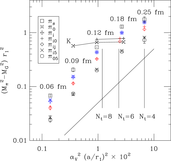
Figure 1: Pion taste splitting relative to the Goldstone pion mass in units of $r_{1}=0.318\,(7)\,(4)$ fm vs. the lattice scaling variable $(a/r_{1})^{2}\alpha_{V}(a)^{2}$ in a log-log plot. Here we take $\alpha_{V}(a)=12\pi/[54\ln[(3.33/a\Lambda)]$ with $\Lambda=319$ MeV. The rising line has slope 1. The fancy diamonds locate the kaon splittings $(m_{K}^{2}-m_{G}^{2})r_{1}^{2}$ for $m_{ud}\approx 0.2\,m_{s}$. The fancy crosses do the same for $m_{ud}\approx 0.1\,m_{s}$. The vertical lines indicate the approximate lattice spacing at the crossover temperature for various $N_{t}$. Data are from Aubin et al. (2004) and unpublished simulation results. The pion taste assignments are given in the gamma matrix basis. The taste singlet is denoted $\pi_{s}$.

It would seem important for studying the strange quark physics of the plasma that the kaon mass be heavier than the pion. In the staggered fermion scheme each meson state appears in a taste multiplet of 16. With improvement of the fermion action the splittings are considerably reduced. The splittings in meson mass squared are expected to vanish in the continuum limit as $a^{2}\alpha_{V}^{2}$. Shown in a log-log plot in Fig. 1 are pion taste splittings relative to the Goldstone pion mass for five lattice spacings. The solid line shows the expected scaling slope. The trend is consistent with the scaling prediction. Shown also are splittings of the lowest member of the kaon multiplet, relative to the Goldstone pion mass for the two choices of $m_{ud}/m_{s}$ in the thermodynamics study. The vertical lines locate the lattice spacing at the crossover temperature $T_{c}$ (about 190 MeV for our unphysical light quark masses) for various $N_{t}$. Note that the temperature then increases as we move to the left. Our nonzero temperature studies are at $N_{t}=4$ and 6. At $N_{t}=4$ the lightest kaon at $T_{c}$ has approximately the same mass as the lowest non-Goldstone pion. As the figure shows, at $N_{t}=4$ the kaon and pion taste multiplets are non-overlapping at approximately $T\geq 2T_{c}$. At the $N_{t}=6$ crossover the situation has improved and the multiplets are non-overlapping at approximately $T\geq 4T_{c}/3$. Clearly, $N_{t}=8$ would be even better for this action.

At $N_{t}=6$ the taste-splitting is about half as large as at $N_{t}=4$. One of our goals was to determine to what extent the increase in $N_{t}$ from 4 to 6 influences the EOS.

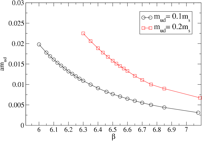
Figure 2: Plot of the two trajectories of constant physics in the $(am_{ud},\beta)$ plane.

In our simulations we use the dynamical $R$ algorithm Gottlieb et al. (1987) with step size equal to the minimum of 0.02 and $2\,am_{ud}/3$. For some runs the step size was chosen to be even smaller. Our aim is to generate zero- and nonzero-temperature ensembles of lattices with action parameters chosen so that a trajectory of constant physics ($m_{\pi}/m_{\rho}={\rm const}$) is approximated. Along the trajectory the heavy quark mass is tuned to the strange quark mass within 20%. We work with two such trajectories: $m_{ud}\approx 0.2\,m_{s}$ ($m_{\pi}/m_{\rho}\approx 0.4$) and $m_{ud}\approx 0.1\,m_{s}$ ($m_{\pi}/m_{\rho}\approx 0.3$) as shown in Fig.  2.

The construction of each trajectory begins with “anchor points” in $\beta$, where the hadron spectrum has been previously studied and the lattice strange quark mass has been tuned to approximate the correct strange hadron spectrum Aubin et al. (2004). We adjusted the value of $am_{ud}$ at the anchor points to give a constant (unphysical) ratio $m_{\pi}/m_{\rho}$. Between these points the trajectory is then interpolated, using a one-loop renormalization-group-inspired formula. That is, we interpolate $\ln(am_{s})$ and $\ln(am_{ud})$ linearly in $\beta$. Since we have three anchor points for the $m_{ud}\approx 0.2\,m_{s}$ trajectory, namely $\beta=6.467$, 6.76, and 7.092, our interpolation is piecewise linear. For the trajectory $m_{ud}\approx 0.1\,m_{s}$ we use two anchor points at $\beta=6.458$ and 6.76. Explicitly the parameterization of the $m_{ud}\approx 0.2\,m_{s}$ trajectory is

$$am_{s} = \left\{\begin{tabular}[]{ll}$0.082\,\exp\left((\beta-6.4674)\frac{\ln(0.050/0.0820)}{(6.76-6.4674)}\right)$,&$\beta\in[6.467,6.76]$\\ $0.05\,\exp\left((\beta-6.76)\frac{\ln(0.031/0.05)}{(7.092-6.76)}\right)$,&$\beta\in[6.76,7.092]$\\ \end{tabular}\right.$$ (9)

$$am_{ud} = \left\{\begin{tabular}[]{ll}$0.01675\,\exp\left((\beta-6.4674)\frac{\ln(0.010/0.01675)}{(6.76-6.4674)}\right),$&$\beta\in[6.467,6.76]$\\ $0.01\,\exp\left((\beta-6.76)\frac{\ln(0.00673/0.01)}{(7.092-6.76)}\right),$&$\beta\in[6.76,7.092].$\\ \end{tabular}\right.$$ (12)

The parameterization of the $m_{ud}\approx 0.1\,m_{s}$ trajectory with $\beta\in[6.458,6.76]$ is

$$am_{s} = 0.05\exp\left((\beta-6.76)\frac{\ln(0.082/0.05)}{(6.458-6.76)}\right)$$ (13)

$$am_{ud} = 0.005\exp\left((\beta-6.76)\frac{\ln(0.0082/0.005)}{(6.458-6.76)}\right).$$ (14)

For both trajectories, for values of $\beta$ out of the interpolation intervals, the parameterization formulae are used to perform extrapolations. The run parameters of the two trajectories at different $N_{t}$ are summarized in Tables 1, 2 and 3. It is apparent from Eqs. (7) and (8) that values of the quark mass ratio $m_{ud}/m_{s}$ in Table 3 deviate slightly from 0.2, since it was our initial intention to keep the hadron masses constant instead. In subsequent practice, as in the $0.1m_{s}$ trajectory, we chose the more convenient alternative of keeping the quark mass ratio fixed.

$\beta$	$am_{ud}$	$am_{s}$	$u_{0}$	$V_{T\neq 0}$	Trajectory	$V_{T=0}$	Trajectory	$a$ [fm]
⋆6.000	0.0198	0.1976	0.8250	$12^{3}\times 4$	1800	$12^{4}$	500	0.366
⋆6.050	0.0178	0.1783	0.8282	$12^{3}\times 4$	1800	$12^{4}$	500	0.334
6.075	0.0169	0.1695	0.8301	$12^{3}\times 4$	1800			0.319
⋆6.100	0.0161	0.1611	0.8320	$12^{3}\times 4$	1800	$12^{4}$	500	0.306
6.125	0.0153	0.1533	0.8338	$12^{3}\times 4$	2800			0.293
⋆6.150	0.0146	0.1458	0.8356	$12^{3}\times 4$	3800	$12^{4}$	500	0.281
6.175	0.0139	0.1388	0.8374	$12^{3}\times 4$	3800			0.269
⋆6.200	0.0132	0.1322	0.8391	$12^{3}\times 4$	3800	$12^{4}$	400	0.258
6.225	0.0126	0.126	0.8407	$12^{3}\times 4$	3800			0.248
⋆6.250	0.012	0.1201	0.8424	$12^{3}\times 4$	3800	$12^{4}$	500	0.238
⋆6.275	0.0114	0.1145	0.8442	$12^{3}\times 4$	2800	$12^{4}$	500	0.229
⋆6.300	0.0109	0.1092	0.8459	$12^{3}\times 4$	1800	$12^{4}$	2100	0.220
⋆6.350	0.00996	0.0996	0.8491	$12^{3}\times 4$	1800	$12^{4}$	2100	0.204
6.400	0.00909	0.0909	0.8520	$12^{3}\times 4$	1800			0.190
⋆6.458	0.0082	0.082	0.8549	$12^{3}\times 4$	1800	$12^{4}$	2100	0.175
6.500	0.00765	0.0765	0.8570	$12^{3}\times 4$	1800			0.165
⋆6.550	0.00705	0.0705	0.8593	$12^{3}\times 4$	1800	$20^{4}$	2100	0.155
6.600	0.0065	0.065	0.8616	$12^{3}\times 4$	1800			0.145
⋆6.650	0.00599	0.0599	0.8636	$12^{3}\times 4$	1800	$24^{4}$	2100	0.137
6.700	0.00552	0.0552	0.8657	$12^{3}\times 4$	1800			0.129
⋆6.760	0.005	0.05	0.8678	$16^{3}\times 4$	800	$24^{3}\times 64$	2100	0.120
⋆6.850	0.00437	0.0437	0.8710	$16^{3}\times 4$	800	$32^{4}$	300	0.109
⋆7.080	0.0031	0.031	0.8779	$16^{3}\times 4$	800	$40^{3}\times 96$	1500	0.086

Table 1: Run parameters of the trajectory with $m_{ud}\approx 0.1\,m_{s}$ at $N_{t}=4$. The asterisk indicates parameter sets for which both zero and nonzero temperature runs were performed. The columns labeled ”Trajectory” indicate the number of thermalized trajectories. Last column shows the lattice spacing as determined from Eq. (15).

$\beta$	$am_{ud}$	$am_{s}$	$u_{0}$	$V_{T\neq 0}$	Trajectory	$V_{T=0}$	Trajectory	$a$ [fm]
⋆6.300	0.0109	0.1092	0.8459	$12^{3}\times 6$	3100	$12^{4}$	2100	0.220
⋆6.350	0.00996	0.0996	0.8491	$12^{3}\times 6$	2900	$12^{4}$	2100	0.204
6.400	0.00909	0.0909	0.8520	$12^{3}\times 6$	2900			0.190
⋆6.458	0.0082	0.082	0.8549	$16^{3}\times 6$	2140	$12^{4}$	2100	0.175
6.500	0.00765	0.0765	0.8570	$12^{3}\times 6$	2900			0.165
⋆6.550	0.00705	0.0705	0.8593	$12^{3}\times 6$	2900	$20^{4}$	2100	0.155
6.600	0.0065	0.065	0.8616	$12^{3}\times 6$	2900			0.145
⋆6.650	0.00599	0.0599	0.8636	$12^{3}\times 6$	2900	$24^{4}$	2100	0.137
6.700	0.00552	0.0552	0.8657	$12^{3}\times 6$	2900			0.129
⋆6.760	0.005	0.05	0.8678	$20^{3}\times 6$	1000	$24^{3}\times 64$	2100	0.120
⋆6.850	0.00437	0.0437	0.8710	$18^{3}\times 6$	1300	$32^{4}$	300	0.109
⋆7.080	0.0031	0.031	0.8779	$18^{3}\times 6$	2200	$40^{3}\times 96$	1500	0.086

Table 2: Same as Table 1 but for trajectory $m_{ud}\approx 0.1\,m_{s}$ at $N_{t}=6$.

$\beta$	$am_{ud}$	$am_{s}$	$u_{0}$	$V_{T\neq 0}$	Trajectory	$V_{T=0}$	Trajectory	$a$ [fm]
⋆6.300	0.0225	0.1089	0.8455	$12^{3}\times 6$	3000	$12^{4}$	2100	0.224
⋆6.350	0.0206	0.1001	0.8486	$12^{3}\times 6$	3000	$12^{4}$	2100	0.208
6.400	0.01886	0.0919	0.8512	$12^{3}\times 6$	3000			0.193
6.433	0.0178	0.087	0.8530	$12^{3}\times 6$	800			0.184
⋆6.467	0.01676	0.0821	0.8549	$16^{3}\times 6$	2200	$16^{3}\times 48$	1225	0.176
6.500	0.0158	0.0776	0.8568	$12^{3}\times 6$	3000			0.168
⋆6.525	0.0151	0.0744	0.8580	$12^{3}\times 6$	3000	$12^{4}$	2100	0.162
6.550	0.0145	0.0713	0.8592	$12^{3}\times 6$	3000			0.157
⋆6.575	0.0139	0.0684	0.8603	$12^{3}\times 6$	3000	$16^{4}$	1760	0.152
6.600	0.0133	0.0655	0.8614	$12^{3}\times 6$	3000			0.147
⋆6.650	0.0121	0.0602	0.8634	$12^{3}\times 6$	3000	$20^{4}$	836	0.138
6.700	0.0111	0.0553	0.8655	$12^{3}\times 6$	3100			0.130
⋆6.760	0.01	0.05	0.8677	$20^{3}\times 6$	1935	$20^{3}\times 64$	825	0.121
⋆6.850	0.00898	0.0439	0.8710	$12^{3}\times 6$	3000	$24^{3}$	740	0.110
7.092	0.00673	0.031	0.8781	$12^{3}\times 6$	3000			0.086
7.090	0.0062	0.031	0.8782			$28^{3}\times 96$	565

Table 3: Same as Table 1 but for trajectory $m_{ud}\approx 0.2m_{s}$ at $N_{t}=6$. The last row is a run which does not lie on the trajectory and was used only for zero-temperature extrapolations.

For the purpose of the EOS determination, the trajectories of constant physics are most conveniently parameterized by the lattice spacing $a$, as discussed at the end of the previous section. To calculate the various derivatives of the bare parameters with respect to $\ln a$ we need to determine the functional dependence $\ln a(\beta)$. The lattice spacing is determined using the method of Ref. Aubin et al. (2004). On a large set of zero-temperature ensembles the static potential is measured to determine the modified Sommer parameter $r_{1}$ Bernard et al. (2000) in lattice units. Specifically, $r_{1}$ is defined by $r_{1}^{2}F_{\bar{q}q}(r_{1})=1$. All available measurements of $r_{1}/a$ are then fit to the following asymptotic-freedom-inspired form Allton (1996, 1997)

$$\frac{a}{r_{1}}=\frac{c_{0}f(g^{2})+c_{2}g^{2}f^{3}(g^{2})+c_{4}g^{4}f^{3}(g^{2})}{1+d_{2}g^{2}f^{2}(g^{2})}.$$ (15)

The definition of

$$f(g^{2})=(b_{0}g^{2})^{-b_{1}/(2b_{0}^{2})}e^{-1/(2b_{0}g^{2})}$$ (16)

involves the universal beta-function coefficients for massless three-flavor QCD, $b_{0}$ and $b_{1}$. The coefficients $c_{0}$, $c_{2}$ and $c_{4}$ are

$$c_{0} = c_{00}+(c_{01u}am_{ud}+c_{01s}am_{s})/f(g^{2})+c_{02}(2am_{ud}+am_{s})^{2}/f^{2}(g^{2})$$

$$c_{2} = c_{20}+c_{21}(2am_{ud}+am_{s})/f(g^{2})$$

$$c_{4} = c_{40}$$

$$d_{2} = d_{20},$$

where $c_{00}=46.766(447)$, $c_{01u}=0.526(122)$, $c_{01s}=0.1817(708)$, $c_{02}=-0.00403(204)$, $c_{20}=-4.702(175)\times 10^{5}$, $c_{21}=3.321(511)\times 10^{3}$, $c_{40}=3.943(84)\times 10^{5}$ and $d_{20}=1.276(484)\times 10^{3}$. The fit has $\chi^{2}/{\rm DoF}\approx 1.3$ and a confidence level of approximately 0.13. This parameterization provides a determination of $r_{1}/a$ along our trajectories of constant physics (Fig. 3).

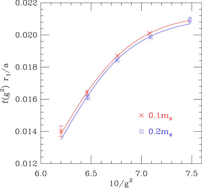
Figure 3: Inverse lattice spacing in units of $f(g^{2})r_{1}$ vs. gauge coupling $\beta=10/g^{2}$, based on the best fit parameterization Eq. (15). The fitting function is evaluated along the two lines of constant physics, namely $m_{ud}\approx 0.1m_{s}$ and $0.2m_{s}$. It is derived from forty measured values of $r_{1}/a$. Eight of them lie on the trajectories of constant physics and are plotted here.

Independently of the fit, the absolute scale for $a$ is set from a determination of the $\Upsilon(2S-1S)$ splitting on a subset of these zero-temperature ensembles Wingate et al. (2004); Gray et al. (2005). An extrapolation to zero lattice spacing then gives $r_{1}=0.318\,(7)\,(4)$ fm Aubin et al. (2004). This value was used in conjunction with the above parameterized value of $r_{1}/a$ to define the physical lattice spacing in our simulations.

IV Equation of State Results and Conclusions

In the previous sections, we have outlined the method we follow to determine the temperature dependence of the bulk thermodynamic quantities, namely, the interaction measure, pressure and energy density, which constitute the EOS for the quark-gluon system. In this section we present our numerical results.

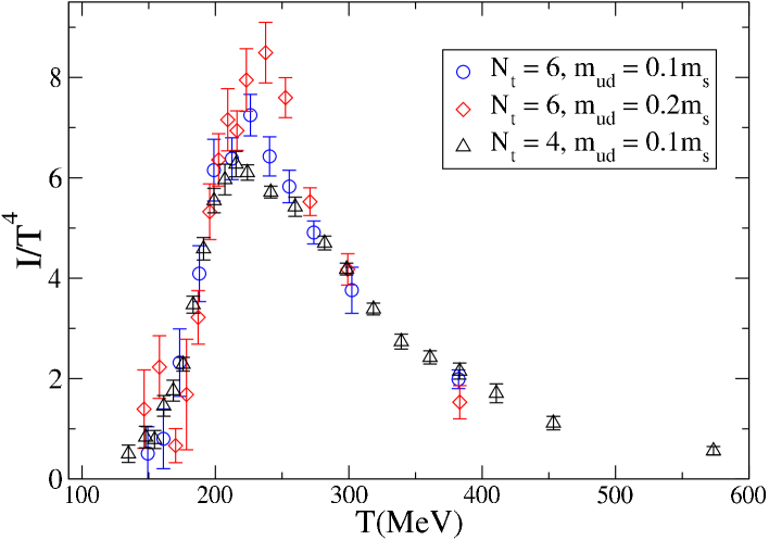
Figure 4: The interaction measure is shown for both of the trajectories of constant physics and the different $N_{t}$.

According to the integral method, at the base of our calculation is the determination of the interaction measure, which is straightforward from Eq. (II). The nonzero temperature value of the interaction measure needs to be corrected for the zero-temperature contributions. This correction is done for about half of the runs by directly measuring the zero-temperature values of the fermionic and gluonic observables involved in Eq. (II) and subtracting their resultant zero-temperature contribution from the interaction measure at nonzero temperature. For the rest of the runs, the zero-temperature correction is calculated by making local interpolations. We need to determine as well the derivatives $d\beta/d\ln a$, $d\beta_{\rm rt}/d\ln a$, $d\beta_{\rm pg}/d\ln a$, $d(m_{f}a)/d\ln a$ and $du_{0}/d\ln a$ for each trajectory. For this purpose we take derivatives of the $\ln(am_{ud})$ and $\ln(am_{s})$ trajectory parameterizations, using Eq. (9) – Eq. (14), polynomial fits to $u_{0}(\beta)$ for both trajectories, and the $a/r_{1}$ fit from Eq. (15). Figure 4 shows the interaction measure as a function of the temperature for both trajectories of constant physics and $N_{t}$’s.

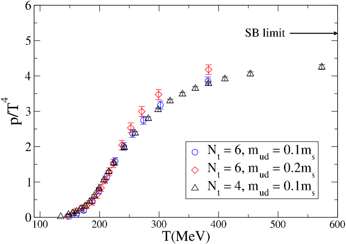
Figure 5: The temperature dependence of the pressure for both of the trajectories of constant physics and the different $N_{t}$. The continuum Stefan-Boltzmann limit for 3 massless flavors is also shown.

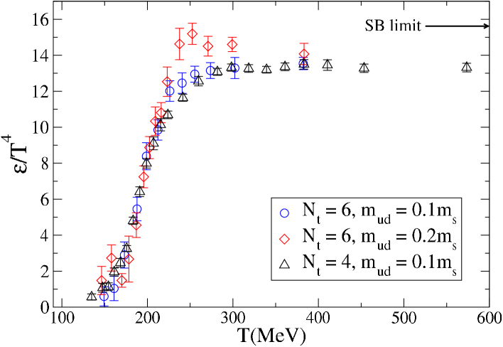
Figure 6: The temperature dependence of the energy density for both of the trajectories of constant physics and the different $N_{t}$. To facilitate comparison with the ideal gas case, the continuum Stefan-Boltzmann limit for 3 massless flavors is also shown.

The pressure is obtained from the interaction measure by integration (Eq. (5)) using the trapezoid method and Fig. 5 shows our results. Using both the interaction measure and the pressure, we calculate the energy density (Eq. (6)). The results are presented in Fig. 6. The statistical errors on all of the thermodynamic quantities are calculated using the jackknife method, and we ignore the insignificant errors on the derivatives of the bare parameters with respect to the lattice scale mentioned above. The EOS data in the Figs. 4 – 6 is corrected for the systematic errors due to the finite step size, which are discussed later in this section and in more detail in the Appendix, and the choice of the lower integration limit in Eq. (5).

From our results for the EOS we find that at the highest studied temperature ($\sim 380$ MeV for $N_{t}=6$ and $\sim 570$ MeV for $N_{t}=4$ ) the energy density is about 10 – 15% below the Stefan-Boltzmann three-flavor limit, which is evidence that strong interactions between the plasma constituents persist in the high temperature phase at several times $T_{c}$. The comparison of the EOS for the two trajectories of constant physics at $N_{t}=6$ shows some small differences. There is a difference in the interaction measure maxima, with the one from the $m_{ud}\approx 0.2\,m_{s}$ trajectory somewhat larger than the $0.1\,m_{s}$ trajectory one. Also, the pressure on the $m_{ud}\approx 0.2\,m_{s}$ trajectory at coarse lattice spacing (see Fig. 5) is gradually becoming slightly larger with temperature than that on the $0.1\,m_{s}$ trajectory. This result is contrary to expectation. We consider that the cause is the accumulation of various systematic errors in the pressure calculation which we discuss later in this section. As a whole, the reduction of the mass of the degenerate light quarks from $m_{ud}\approx 0.2\,m_{s}$ to $0.1\,m_{s}$ does not affect dramatically the basic thermodynamic properties of the system. We see a lot of similarity between the EOS at $N_{t}=4$ and 6 for the $m_{ud}\approx 0.1\,m_{s}$ trajectory. The main differences between the two available $N_{t}$ results is again in the interaction measure, where the maximum at $N_{t}=6$ is higher. Although the discretization artifacts at $N_{t}=4$ are known to be larger than in the $N_{t}=6$ case, we find that their effect on the EOS is not very pronounced.

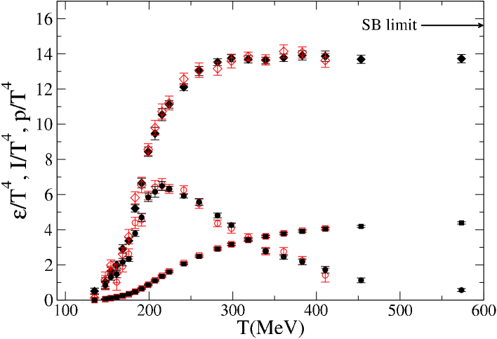
Figure 7: Volume dependence of results for $N_{t}=4$ with $m_{ud}\approx 0.1m_{s}$. Empty symbols are used for small volume ($V_{s}=8^{3}$) results, and filled symbols are used for large volume ($V_{s}=12^{3}$ or $16^{3}$) results. The energy density, pressure and interaction measure are plotted using diamonds, squares and circles, respectively. The data are not corrected for any systematic errors. We see no statistically significant volume dependence.

Our EOS calculation can be affected by the following systematic errors: finite volume effects, finite step-size effects, the error in the determination of the lower integration limit in Eq. (5), possible deviations from the trajectories of constant physics and the uncertainties in the scale determination from Eq. (15). First we discuss the scale determination error. The lattice spacing is most difficult to obtain for the $N_{t}=4$ case in the low temperature region, where the lattices are coarse. We have estimated that a 5% error on the lattice scale there gives up to a three-sigma effect in the region of the interaction measure maximum. This translates as well into up to two-sigma effects on the energy density and pressure at high temperatures, since errors accumulate in the integration needed to obtain these quantities.

To address the question of the finite volume effects we have conducted a set of runs at $N_{t}=4$ with parameters from the $m_{ud}\approx 0.1\,m_{s}$ trajectory on lattices with smaller spatial volume – $V_{s}=8^{3}$. In Fig. 7 the thermodynamic quantities calculated using $V_{s}=8^{3}$ are compared with the ones on the larger spatial volumes – $V_{s}=12^{3},16^{3}$. We find no statistically significant difference which leads us to conclude that in our calculation the finite volume effects are negligible.

The determination of the lower integration limit in Eq. (5) is potentially another source of systematic error. The lowest available temperature in our calculations is around 135 MeV at $N_{t}=4$, and 149 MeV at $N_{t}=6$. To estimate the pressure at these temperatures we calculate the pressure of an ideal Bose gas of pions with masses similar to those in our simulations. The true Goldstone pions on the physics trajectories have mass of $\sim 270$ MeV and the rest of the members of the pion multiplet are heavier. We estimated the heavy pion masses using extrapolations of available data for the taste splitting in the pion multiplet, summarized in Fig. 1. Including all of the pions according to their degeneracy, we estimate $p/T^{4}(T=135\,\,{\rm MeV})\sim 0.02$ and $p/T^{4}(T=149\,\,{\rm MeV})\sim 0.03$ with about 30% uncertainty in these values. Both of these estimations are comparable or a bit larger than the size of the statistical error on the pressure at the closest available low temperatures. Consequently we have corrected the pressure and energy density by adding them to the data. At high temperatures this correction is smaller than the statistical error.

The error due to deviations from the trajectories of constant physics would be largest in the $N_{t}=4$ case, for which the points around the transition region and at lower temperature were obtained by extrapolations using Eqs. (9) and (10). Indeed, a later spectrum calculation near the transition, at $\beta=6.2$, showed that there is about a 10% difference from the target value for $m_{\pi}/m_{\rho}$. However, considering that the differences between the two $N_{t}=6$ trajectories, for which $m_{\pi}/m_{\rho}$ differs by about 30%, is no more than four sigma, we estimate the effect at about one sigma in the transition region and smaller outside of it.

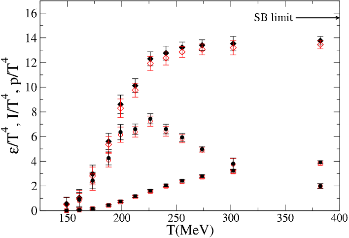
Figure 8: Effect of step-size corrections for $N_{t}=6$ with $m_{ud}\approx 0.1m_{s}$. We use filled (open) symbols to plot uncorrected (corrected) results. The symbols for the energy density, pressure and interaction measure are diamonds, squares and circles, respectively.

The last potentially significant source of systematic error is the finite step size used in the $R$ algorithm. For $N_{t}=4$ and 6 we have carried out a set of test simulations at a larger step size in the $R$ algorithm to estimate their effect. In addition we have performed some RHMC Clark et al. (2005) calculations to complement our finite step-size study. Our analysis of the results is presented in the Appendix. We find that the effect of the step-size corrections to the gauge observables on the interaction measure is no larger than the size of our statistical error along the $m_{ud}\approx 0.1\,m_{s}$ trajectory and negligible along the $m_{ud}\approx 0.2\,m_{s}$ one. The effects of the correction to the fermionic observables for both trajectories is small enough to be ignored. We use the empirical formula in Eq. (17) with the parameters in Eq. (18) to compute the correction to the three gauge loop observables for the $m_{ud}\approx 0.1\,m_{s}$ trajectory only. We do not correct the $m_{ud}\approx 0.2\,m_{s}$ trajectory for finite step-size effects due to their smallness. Figure 8 shows the EOS for the $m_{ud}\approx 0.1\,m_{s}$, $N_{t}=6$ case with the finite step-size correction compared with the uncorrected case. The correction is no larger than our statistical errors. As explained in the appendix, we estimate the uncertainty in the correction itself to be about 50%.

Appendix A Step-size dependence of EOS observables

With the $R$ algorithm the integration step size in the molecular dynamics evolution must be chosen small enough to achieve the desired accuracy in observables of interest. For most practical purposes we have found errors at our standard small production step sizes to be insignificant. (For a recent test see Table IX of Aubin et al. (2004).) However, the observables required for the equation of state must be measured to a very high accuracy, since the small differences between the hot and cold measurements are sensitive to even small systematic errors. The most important observable in this regard is the plaquette. For the present study we have developed a rough empirical method for estimating and correcting for these errors in our simulations.

To estimate the step-size error within the $R$ algorithm requires carrying out simulations at a range of step sizes and determining the change in the observable as the step size tends to zero. We have carried out a number of such tests on hot and cold Asqtad lattices, measuring most of the observables needed for the equation of state. The RHMC algorithm, which we incorporated into our code at the end of this study, does not suffer from such step size errors. Thus for the purpose of modeling step-size corrections we include results of some RHMC calculations. For our previous study of the equation of state with the unimproved gauge action and naive staggered fermion action, we made extensive measurements of the step-size dependence of the plaquette and chiral condensate Bernard et al. (1997).

The leapfrog-inspired $R$ algorithm is specifically designed to be a second order integration algorithm. That is, the truncation error at the end of a molecular dynamics trajectory of fixed length decreases with the integration step size $\epsilon$ as $\epsilon^{2}$. In Figs. 9 and 10 we show the step-size dependence of the plaquette and chiral condensate for the improved action for one pair of ensembles. On the larger-volume zero-temperature lattices, we have found that the variation of the plaquette with decreasing step size shows more apparent curvature over this range of step sizes than do the smaller volume high temperature lattices. Consequently, as shown, we fit the low temperature results to a quadratic in $\epsilon^{2}$. Clearly both low and high temperature values are subject to correction. The corrections tend to cancel in the difference. For the improved action the slopes for all seven observables needed for the equation of state are tabulated in Tables 4 and 5. For the high temperature ensembles the slope is determined by a linear fit in $\epsilon^{2}$. For the zero temperature ensembles it is determined from results at our smallest available pair of values of $\epsilon^{2}$, treating an RHMC step size as 0, of course.

Figure 9: Plaquette (left panel) and chiral condensate (right panel) vs the squared step size $\epsilon^{2}$ for the improved action for the ensemble at $\beta=6.458$, $am_{ud}=0.0082$ and $am_{s}=0.082$. The squared step size for the production of this ensemble is 0.00003

Figure 10: Same as Fig. 9 but for the ensemble at $\beta=6.467$, $am_{ud}=0.01676$ and $am_{s}=0.0821$. The squared step size for the production of this ensemble is 0.0001

The step-size correction depends largely on the size of the fermion force, which is computed by inverting the fermion matrix. Small eigenvalues dominate the inverse. The smallest eigenvalue is controlled by the light quark mass. Since the chiral condensate is also determined from the inverse of the fermion matrix, we would expect the chiral condensate and light quark mass to be natural parameters for the step size error regardless of temperature. Consequently, along a chosen trajectory of constant physics, we parameterize the step-size slope of the plaquette for both high and low temperature ensembles as a polynomial in the chiral condensate. For the $m_{ud}\approx 0.1\,m_{s}$ trajectory we find it is modeled reasonably well by the following quadratic form as shown in Fig. 11:

$$\frac{dP}{d\epsilon^{2}}=b(x-0.1)^{2}+m(x-0.1)+c,$$ (17)

where $x=a^{3}\langle\bar{\psi}\psi\rangle_{ud}$ is the light quark chiral condensate in lattice units.

Figure 11: Plaquette slopes for the $m_{ud}\approx 0.1\,m_{s}$ trajectory (left) and the $m_{ud}\approx 0.2\,m_{s}$ trajectory (right) vs. the chiral condensate. On the left panel the quadratic fit to the data, Eq (17), is shown as well. Squares, diamonds, and octagons indicate slopes determined from two different R algorithm step sizes. Fancy squares, fancy diamonds, and bursts indicate slopes determined by comparing R- with RHMC-algorithm measurements.

The best fit values are

$$b = 250(177),\ \ m=-109(54),\ \ c=-6.1(2.7),$$ (18)

for $\chi^{2}/df=23/11$. Thus our empirical model explains most of the observed variation but not all. We use it to estimate the step-size correction along the $m_{ud}\approx 0.1\,m_{s}$ trajectory. By comparison the plaquette slopes for the $m_{ud}\approx 0.2\,m_{s}$ trajectory are small. If we apply a correction according to a crude linear fit to these slopes, the effect on the EOS is much smaller than our statistical errors. For these reasons we chose to ignore the step-size error for this trajectory.

The fit to the step size correction also allows us to estimate the error in our ability to predict the correction. The largest error, approximately 50%, occurs at small values of the chiral condensate. We take this as a conservative estimate of the error in our correction throughout.

Table 4 shows, not surprisingly, that the variation in all three gauge loop observables is correlated. With our normalization the slopes appear to be of comparable magnitude. This observation suggests generalizing the absolute plaquette correction to all three gauge loops.

We also tabulate the slope of the fermion variables in Table 5. Except for the gauge contribution, all other estimated corrections to the EOS are negligible compared with our statistical errors. The gauge-action correction is smaller than our statistical error in most cases; however, we have included it in the EOS for the $m_{ud}\approx 0.1\,m_{s}$ trajectory since, although its effect is comparable to the statistical error, it lowers all data points consistently.

volume	$\beta$	$am_{ud}$	$am_{s}$	$\left\langle P\right\rangle$	$\left\langle R\right\rangle$	$\left\langle C\right\rangle$
R $12^{3}\times 4$	6.0	0.0198	0.1976	$-$14(5)	$-$12(6)	$-$8(7)
R $12^{3}\times 4$	6.1	0.0161	0.1611	$-$24(8)	$-$25(9)	$-$25(10)
R $12^{3}\times 4$	6.2	0.0132	0.1322	$-$18(7)	$-$22(8)	$-$21(10)
R $12^{3}\times 12$	6.2	0.0132	0.1322	$-$25(5)	$-$26(5)	$-$26(7)
H $16^{3}\times 48$	6.35	0.00996	0.0996	$-$5(4)	$-$5(6)	$-$5(7)
H $16^{3}\times 48$	6.35	0.0206	0.1001	$-$0.6(1.3)	$-$1.0(1.6)	$-$1.3(1.9)
H $16^{3}\times 48$	6.40	0.00909	0.0909	$-$17(4)	$-$20(5)	$-$17(4)
H $16^{3}\times 48$	6.40	0.01886	0.0909	4(3)	5(3)	5(4)
R $12^{3}\times 4$	6.458	0.0082	0.082	$-$11(6)	$-$14(8)	$-$20(9)
H $16^{3}\times 6$	6.458	0.0082	0.082	$-$18(4)	$-$18(4)	$-$13(11)
H $16^{3}\times 48$	6.458	0.0082	0.082	$-$11(4)	$-$11(7)	$-$14(7)
H $16^{3}\times 6$	6.467	0.01676	0.0821	$-$3.8(1.6)	$-$5(2)	$-$5(3)
H $16^{3}\times 48$	6.467	0.01676	0.0821	2.1(1.4)	3(2)	4(2)
H $16^{3}\times 48$	6.50	0.00765	0.0765	$-$6(5)	$-$5(6)	$-$4(7)
R $12^{3}\times 6$	6.55	0.00705	0.0705	1.4(9)	4(14)	6(13)
R $12^{3}\times 12$	6.565	0.005	0.0484	$-$36(4)	$-$46(6)	$-$48(6)
R $12^{3}\times 6$	6.65	0.00599	0.0599	5(10)	1(13)	5(11)
H $12^{3}\times 4$	6.76	0.005	0.082	22(11)	19(18)	23(16)
R $24^{3}\times 64$	6.76	0.005	0.05	$-$11(2)	$-$15(3)	$-$10(3)
R $20^{3}\times 6$	6.76	0.01	0.05	5(2)	4(4)	4(3)
R $20^{3}\times 64$	6.76	0.01	0.05	$-$1.8(6)	$-$2.9(4)	$-$2.6(6)
R $20^{3}\times 64$	6.79	0.02	0.05	1.24(12)	1.12(14)	1.23(10)
R $20^{3}\times 64$	6.81	0.03	0.05	2.04(7)	2.04(9)	2.09(10)

Table 4: Step-size slope $d{\cal O}/d\epsilon^{2}$ for gauge field contributions to the equation of state for a variety of lattice ensembles. Three operators ${\cal O}$ are tabulated. The label R indicates values determined exclusively from the $R$ algorithm. The label H indicates values determined with the aid of the RHMC algorithm.

volume	$am_{ud}$	$\langle\bar{\psi}\psi\rangle_{ud}$	$\langle\bar{\psi}\psi\rangle_{s}$	$\left\langle\bar{\psi}\frac{dM}{du_{0}}\psi\right\rangle_{ud}$	$\left\langle\bar{\psi}\frac{dM}{du_{0}}\psi\right\rangle_{s}$
R $12^{3}\times 4$	0.0198	3(10)	4(5)	27(20)	45(19)
R $12^{3}\times 4$	0.0161	26(21)	19(11)	66(40)	70(37)
R $12^{3}\times 4$	0.0132	39(36)	26(16)	53(32)	54(29)
R $12^{3}\times 12$	0.0132	15(11)	17(5)	44(17)	75(17)
H $16^{3}\times 48$	0.00996	$-$35(14)	$-$4(8)	12(16)	13(17)
H $16^{3}\times 48$	0.0206	$-$2(2)	$-$1(2)	1(5)	0(5)
H $16^{3}\times 48$	0.00909	$-$3(9)	3(41)	0(18)	0(18)
H $16^{3}\times 48$	0.01886	$-$15(5)	$-$7(4)	7(7)	12(7)
R $12^{3}\times 4$	0.0082	1.6(1.4)	9(6)	27(19)	45(19)
H $16^{3}\times 6$	0.0082	5(16)	10(8)	36(11)	44(12)
H $16^{3}\times 48$	0.0082	$-$2(10)	3(5)	$-$	$-$
H $16^{3}\times 6$	0.01676	$-$13(4)	$-$4(3)	11(2)	11(2)
H $16^{3}\times 48$	0.01676	0.7(8)	1.8(7)	9(3)	7(3)
H $16^{3}\times 48$	0.00765	$-$5(10)	$-$5(8)	$-$3(15)	15(14)
R $12^{3}\times 6$	0.00705	$-$20(25)	$-$18(23)	$-$16(25)	$-$6(24)
R $12^{3}\times 12$	0.005	$-$5(9)	18(6)	$-$	$-$
R $12^{3}\times 6$	0.00599	19(12)	33(20)	10(22)	5(30)
H $12^{3}\times 4$	0.005	0.2(4)	0.7(3)	$-$30(28)	$-$73(27)
R $24^{3}\times 64$	0.005	5.4(1.8)	1.1(1.6)	$-$6.9(2.9)	$-$2.7(3.3)
R $20^{3}\times 6$	0.01	$-$1.5(1.3)	$-$2.7(2.7)	$-$12(5)	$-$6(7)
R $20^{3}\times 64$	0.01	$-$0.6(9)	1.2(6)	$-$	$-$
R $20^{3}\times 64$	0.02	$-$1.1(3)	$-$1.2(2)	$-$	$-$
R $20^{3}\times 64$	0.03	$-$0.66(11)	$-$0.61(9)	$-$	$-$

Table 5: Step-size slope $d{\cal O}/d\epsilon^{2}$ for fermion contributions to the equation of state for the ensembles of Table 4. Four operators ${\cal O}$ are tabulated.

References

- Adcox et al. (2005) K. Adcox et al., Nucl.Phys. A 757, 184 (2005), eprint [nucl-ex/0410003].
- Huovinen and Ruuskanen (2006) P. Huovinen and P. V. Ruuskanen (2006), eprint [nucl-th/0605008].
- Hindmarsh and Philipsen (2005) M. Hindmarsh and O. Philipsen, Phys. Rev. D71, 087302 (2005), eprint [hep-ph/0501232].
- Blum et al. (1995) T. Blum, L. Karkkainen, D. Toussaint, and S. A. Gottlieb, Phys. Rev. D51, 5153 (1995), eprint [hep-lat/9410014].
- Karsch et al. (2000) F. Karsch, E. Laermann, and A. Peikert, Phys. Lett. B478, 447 (2000), eprint [hep-lat/0002003].
- Engels et al. (1997) J. Engels et al., Phys. Lett. B396, 210 (1997), eprint [hep-lat/9612018].
- Bernard et al. (2005) C. Bernard et al., PoS LAT2005, 156 (2005), eprint [hep-lat/0509053].
- Aoki et al. (2006) Y. Aoki, Z. Fodor, S. D. Katz, and K. K. Szabo, JHEP 01, 089 (2006), eprint [hep-lat/0510084].
- Bernard et al. (2006) C. Bernard et al., PoS LAT2006, 139 (2006), eprint [hep-lat/0610017].
- Engels et al. (1990) J. Engels, J. Fingberg, F. Karsch, D. Miller, and M. Weber, Phys. Lett. B252, 625 (1990).
- Orginos and Toussaint (1998) K. Orginos and D. Toussaint (MILC), Phys. Rev. D59, 014501 (1998), eprint [hep-lat/9805009].
- Toussaint and Orginos (1999) D. Toussaint and K. Orginos (MILC), Nucl. Phys. Proc. Suppl. 73, 909 (1999), eprint [hep-lat/9809148].
- Lepage (1999) G. P. Lepage, Phys. Rev. D59, 074502 (1999), eprint [hep-lat/9809157].
- Aubin et al. (2004) C. Aubin et al., Phys. Rev. D70, 094505 (2004), eprint [hep-lat/0402030].
- Gottlieb et al. (1987) S. A. Gottlieb, W. Liu, D. Toussaint, R. L. Renken, and R. L. Sugar, Phys. Rev. D35, 2531 (1987).
- Bernard et al. (2000) C. W. Bernard et al., Phys. Rev. D62, 034503 (2000), eprint [hep-lat/0002028].
- Allton (1996) C. R. Allton (1996), eprint [hep-lat/9610016].
- Allton (1997) C. R. Allton, Nucl. Phys. Proc. Suppl. 53, 867 (1997), eprint [hep-lat/9610014].
- Wingate et al. (2004) M. Wingate, C. T. H. Davies, A. Gray, G. P. Lepage, and J. Shigemitsu, Phys. Rev. Lett. 92, 162001 (2004), eprint [hep-ph/0311130].
- Gray et al. (2005) A. Gray et al., Phys. Rev. D72, 094507 (2005), eprint [hep-lat/0507013].
- Clark et al. (2005) M. A. Clark, A. D. Kennedy, and Z. Sroczynski, Nucl. Phys. Proc. Suppl. 140, 835 (2005), eprint [hep-lat/0409133].
- Bernard et al. (1997) C. W. Bernard et al. (MILC), Phys. Rev. D55, 6861 (1997), eprint [hep-lat/9612025].