We review a number of topics related to block variable renormalisation group transformations of quantum fields on the lattice, and to the emerging perfect lattice actions. We first illustrate this procedure by considering scalar fields. Then we proceed to lattice fermions, where we discuss perfect actions for free fields, for the Gross-Neveu model and for a supersymmetric spin model. We also consider the extension to perfect lattice perturbation theory, in particular regarding the axial anomaly and the quark gluon vertex function. Next we deal with properties and applications of truncated perfect fermions, and their chiral correction by means of the overlap formula. This yields a formulation of lattice fermions, which combines exact chiral symmetry with an optimisation of further essential properties. We summarise simulation results for these so-called overlap-hypercube fermions in the two-flavour Schwinger model and in quenched QCD. In the latter framework we establish a link to Chiral Perturbation Theory, both, in the $p$-regime and in the $\epsilon$-regime. In particular we present an evaluation of the leading Low Energy Constants of the chiral Lagrangian — the chiral condensate and the pion decay constant — from QCD simulations with extremely light quarks.

Motivation and Overview

Over the recent decades quantum field theory has been established as the appropriate formalism for particle physics, as far as it is explored experimentally. Its treatment by perturbation theory led to successful results, for instance in Quantum Electrodynamics (QED), in the electroweak sector of the Standard Model and in Quantum Chromodynamics (QCD) at high energy. However, there are still many open questions, which require results at finite coupling strength — beyond the range of perturbation theory — such as numerous aspects of QCD at low and moderate energy.

A method is known which has the potential to provide fully non-perturbative results for a number of field theoretic questions. This method applies Monte Carlo simulations to lattice regularised quantum field theories. The generic uncertainty of perturbation theory — uncontrolled contributions beyond the calculated order — disappears in this approach. However, one has to deal with statistical errors, as well as ambiguities in the extrapolation to the continuum and to a large volume.

Simulation results are obtained at finite lattice spacing, which causes systematic artifacts in the numerically measured observables. The stability of dimensionless ratios of observables under the variation of the lattice spacing is denoted as the scaling behaviour. Its quality, which is vital for the reliability of the continuum extrapolation, depends on the way in which the lattice regularisation is implemented. This work deals with renormalisation group techniques to improve the scaling behaviour compared to the standard lattice formulations, which describes, for instance, derivatives simply by differences between nearest neighbour lattice sites. In contrast to Symanzik’s program, this technique does not attempt to correct a specific order in the lattice spacing, but it directly addresses a finite cutoff. We describe the renormalisation group approach in detail and present a variety of results that it led to, in particular for fermionic systems.

The symmetries of a model under consideration are a key aspect for a controlled continuum extrapolation. A great virtue of the lattice regularisation is the conservation of exact gauge symmetries. But global symmetries are often explicitly broken by the lattice structure, for instance the continuous Poincaré invariance. The question, how well — and if — they are restored as we approach the continuum limit is a notorious issue, which is related to the scaling behaviour. Again it depends on the features of the lattice formulation, i.e. on the extent of the explicit symmetry breaking due to a finite lattice spacing. The renormalisation group technique provides a tool to improve the symmetries on the regularised level — in principle they can even be implemented exactly — which renders the continuum limit smoother and safer. This property is particularly relevant for the (approximate) chiral symmetry of (almost) massless fermions. The chiral symmetry is essential for instance in QCD at low energy, and its discussion will take a central rôle in this work. Here we also need a chiral extrapolation, in addition to the limits that we mentioned already.

As an introduction, we summarise in Section 1 some basic aspects of quantum field theory in the functional integral formulation. In particular we sketch the road from classical mechanics to Euclidean quantum field theory, with quantum mechanics and classical field theory as intermediate steps. We focus on the lattice regularisation, which we first introduce for the case of scalar fields. This allows us to summarise the notions and notations used throughout this work.

In Section 2 we describe — still for scalar fields — the concept of block variable renormalisation group transformations. Under iteration they lead to a perfect lattice action, which is free of any cutoff artifacts. We also encounter approximations to a perfect action, which are needed for practical purposes, such as the classical perfection and the truncation of the couplings. Still the lattice artifacts can be kept small for such approximations, as we illustrate for the dispersion relation, the topological susceptibility of a quantum rotor and for thermodynamic quantities.

In Section 3 we proceed to fermionic quantum field theories, where we start again with a few generalities. We review the traditional formulations of lattice fermions and describe the doubling problem. It is related to the difficulty to keep track of the chiral symmetry in a regularised system — an obstacle, which obstructs other regularisation schemes as well. Therefore the existence of light quarks is an amazing feature of Nature, which cannot be described easily in a natural way. In that context, we discuss a brane world scenario as a possible solution to this hierarchy problem.

Section 4 applies the concept of perfect actions to lattice fermions, which takes us to the main topic of this work. For free fermions, we demonstrate that this approach provides both, a solution to the doubling problem and at the same time an exact scaling behaviour. Depending on the choice of the renormalisation group transformation, we can implement either locality or standard chirality in the perfect lattice action. However, if we insist on locality, the resulting Dirac operator still obeys the Ginsparg-Wilson relation, which guarantees a lattice modified but exact chiral symmetry.

In principle, exact scaling and chirality can also be realised at finite lattice spacing in the interacting case, where, however, perfect actions can in general not be constructed explicitly. An exception is the Gross-Neveu model in the limit of a large number of flavours. Here we present a perfect action for staggered fermions, and we approve the perfect scaling for the ratio of the chiral condensate and the dynamically generated fermion mass. The concept we are dealing with also reaches out to perfect lattice currents. With that ingredient, perfect actions can even capture exact supersymmetry on the lattice.

In Section 5 we consider perfect lattice perturbation theory. We give results for the anharmonic oscillator and the Yukawa term, which couples fermions to a scalar field. In lattice gauge theory we show that the perfect lattice action retrieves correctly the axial anomaly, and we discuss the quark gluon vertex function in QCD.

For practical applications, i.e. for the applicability in simulations, the couplings have to be truncated. In Section 6 we describe our truncation scheme for the perfect fermion to a so-called hypercube fermion, which has been simulated successfully in the Schwinger model. In QCD it has been used for the spectral functions at finite temperature, and — together with a truncated perfect vertex function — in the evaluation of the charmonium spectrum. For truncated perfect fermions, the scaling behaviour and chirality are not exact anymore, but the latter can be corrected again by inserting the hypercube fermion into the overlap formula.

This procedure yields the “overlap hypercube fermion”, which is an exact solution to the Ginsparg-Wilson relation. Its construction and properties are presented in Section 7. Similarly we can arrange for a modified but exact parity symmetry for lattice fermions in three dimensions. In two dimensions we review simulations results for overlap hypercube fermions in the two-flavour Schwinger model, which reveal an excellent scaling behaviour. Here and also in QCD we further observe a strongly improved level of locality and approximate rotation symmetry compared to the standard overlap fermion.

Section 8 finally presents simulation results with Ginsparg-Wilson fermions in QCD, using the overlap hypercube fermion as well as the standard formulation of overlap fermions, both in the quenched approximation. This enables simulations near the chiral limit. Here our main goal is a connection to Chiral Perturbation Theory. This is an effective theory of strong interactions at low energy, which provides a variety of successful predictions. However, its effective Lagrangian involves free parameters denoted as the Low Energy Constants, which play an important rôle in the physics of light mesons. Their theoretical determination can only emerge from QCD as the fundamental theory. This is a challenge for lattice simulations, and the principal issue of Section 8.

We measured light meson masses in the $p$-regime (characterised by a large volume), and we reveal the difficulties to evaluate Low Energy Constants in that setting. Then we focus our interest on the $\epsilon$-regime, which deals with a small volume. In the $\epsilon$-regime, the topological sectors play an extraordinary rôle. Hence we first give results for the distribution of topological charges and the resulting susceptibility, which is relevant for the mass of the $\eta^{\prime}$ meson. Next we describe a 3-loop calculation which confirms the perturbative renormalisability of the $\epsilon$-expanded effective theory. We then apply various techniques to extract the leading Low Energy Constants: the chiral condensate — which is the order parameter of chiral symmetry breaking — and the phenomenologically known pion decay constant. In particular, the density of low lying eigenvalues of the Dirac operator is fitted to predictions by chiral Random Matrix Theory. The axial-vector current correlator, as well as the zero-mode contributions to the pseudoscalar density correlation, are confronted with formulae of quenched Chiral Perturbation Theory. We will see that these methods do have the potential to evaluate the Low Energy Constants with their phenomenological values — which correspond to the large volume limit — even in the $\epsilon$-regime. However, the final results have to await the feasibility of dynamical QCD simulations with chiral quarks.

Section 9 is dedicated to concluding remarks, summarising the status of the fields of research that we addressed, along with an outlook on future perspectives.

1 Introduction

1.1 From classical mechanics to quantum mechanics

In classical mechanics, the trajectory $\vec{x}(t)$ of a point particle between fixed endpoints $\vec{x}(0)$ and $\vec{x}(T)$ is — in simple situations — determined by the principle of least action, which imposes the condition $\delta S=0$. The action $S[x]$ is a functional of the conceivable particle paths $\vec{x}(t)$,

$$S[x]=\int_{0}^{T}dt\,L(\vec{x},\dot{\vec{x}})\ ,$$ (1.1)

where $L$ is the Lagrange function. A simple form of it reads

$$L(\vec{x},\dot{\vec{x}})=\frac{m}{2}\dot{\vec{x}}(t)^{\,2}-V(\vec{x}(t))\ ,$$ (1.2)

with the particle mass $m$ and a potential $V$ (which we assume to be velocity independent). The variational condition $\delta S=0$ corresponds to Newton’s equation of motion, $m\ddot{\vec{x}}=-\nabla V$, at each instant $t\in[0,T]$.

Let us consider this transition in quantum mechanics. In contrast to classical mechanics, we now deal with a transition amplitude, which picks up contributions from all possible paths connecting the fixed endpoints. Hence the path in between is not determined. These contributions are summed up coherently,

$$\langle\vec{x}(T)|\vec{x}(0)\rangle=\int{\cal D}x\,\exp\Big{(}\frac{i}{\hbar}S[x]\Big{)}\ .$$ (1.3)

This expression represents a path integral (or functional integral), where the functional measure ${\cal D}x$ symbolises the summation over all possible paths (which formally requires an infinite dimensional integral) [1].

In the (hypothetical) limit $\hbar\to 0$ solely the classical path (which we assume to be unique) contributes, whereas the additional contributions for $\hbar>0$ correspond to the quantum effects. However, if a path far from the classical one is varied, the phase in eq. (1.3) tends to rotate rapidly, so that such contributions almost cancel. As long as $\hbar$ is small compared to the action shift caused by path variations on the scale of interest, it is the vicinity of the classical path that dominates the transition amplitude (1.3).

This situation has a historically older counterpart in optics, where the classical and the quantum mechanical description correspond to the principles by Fermat and by Huygens, respectively.

In order to attribute an explicit meaning to the functional measure ${\cal D}x$, we divide the period $T$ into $N$ equidistant intervals of length $a=T/N$. In this discretised system, the path integral is given by $N-1$ integrals over the possible positions at the times $t_{j}=j\cdot a$, $j=1\dots N-1$. The expression (1.3) is then understood as the continuum extrapolation $a\to 0$ (which, at fixed $T$, corresponds to $N\to\infty$),

$$\prod_{j=1}^{N-1}\int_{{{\kern 1.75pt\sf{R}\kern-4.20004pt\sf{I}\kern 4.20004pt\kern-1.75pt}}^{3}}d^{3}x_{j}\ \dots\quad\ ^{a\to 0}_{\longrightarrow}\qquad\int{\cal D}x\ \dots$$ (1.4)

1.2 Classical field theory

In field theory we do not consider particle paths $\vec{x}(t)$, but instead fields $\phi(x)$, where $x=(t,\vec{x})$ is a point in space-time. The (classical) field takes its value in some abstract space, like ${\kern 2.5pt\sf{R}\kern-7.79999pt\sf{I}\kern 7.79999pt\kern-2.5pt}^{n}$ or ${\kern 2.5pt\sf{C}\kern-4.49997pt\sf{I}\kern 4.49997pt\kern-2.5pt}^{n}$, for example. Now space and time are treated on an equal footing (up to the signature in the metrics), which is a prerequisite for covariance. Moreover, the number of degrees of freedom is extended drastically: before there were just three of them (in each time point $t$), but now there is a degree of freedom for each field component in each single space-time point $x$.

We assume in each point $x$ a Lagrange density ${\cal L}(\phi,\partial_{\mu}\phi)$ to be defined ($\mu=0,\dots,3$), which we denote as the Lagrangian. The field theoretic action is given by

$$S[\phi]=\int d^{4}x\,{\cal L}(\phi,\partial_{\mu}\phi)\ .$$ (1.5)

Now an action value is obtained for each field configuration $\phi(x)$. This means that $S$ is a functional of the fields involved, which take the rôle of the paths in the mechanical system.

The simplest case is a neutral scalar field $\phi(x)\in{\kern 2.5pt\sf{R}\kern-7.79999pt\sf{I}\kern 7.79999pt\kern-2.5pt}$. If this field describes free scalar particles of mass $m$, its Lagrangian reads

$${\cal L}(\phi,\partial_{\mu}\phi)=\frac{1}{2}\partial_{\mu}\phi(x)\partial^{\mu}\phi(x)-\frac{m^{2}}{2}\phi(x)^{2}\ .$$ (1.6)

Assembling the Lagrangian ${\cal L}$ only by covariant terms — as it is the case in eq. (1.6) — ensures that we are dealing with relativistic field theories.

In classical field theory the configuration is determined by again enforcing the variational condition $\delta S=0$. For a neutral scalar field, this implies

$$\frac{\partial{\cal L}}{\partial\phi}-\partial_{\mu}\frac{\partial{\cal L}}{\partial(\partial_{\mu}\phi)}=0\ ,$$ (1.7)

which translates for the Lagrangian (1.6) into the Klein-Gordon equation of motion for the scalar field,

$$[\,\partial_{\mu}\partial^{\mu}-m^{2}\,]\,\phi(x)=0\ .$$ (1.8)

In simple situations, the variational principle and the boundary conditions fix the classical field configuration $\phi(x)$ everywhere in space-time.

As a well-known example, electrodynamics deals with vector fields ${\cal A}_{\mu}(x)$, which represent the electromagnetic potentials. The Lagrangian

$${\cal L}=-\frac{1}{4}F_{\mu\nu}F^{\mu\nu}+j_{\mu}{\cal A}^{\mu}\ ,\quad F_{\mu\nu}=\partial_{\mu}{\cal A}_{\nu}-\partial_{\nu}{\cal A}_{\mu}\ ,$$ (1.9)

is constructed from the (gauge invariant) field strength tensor $F_{\mu\nu}$, and we added an external, electrically charged current $j_{\mu}(x)$. Now the condition $\delta S=0$ leads to the inhomogeneous Maxwell equations

$$\partial_{\mu}F^{\mu\nu}=j^{\nu}\ ,$$

from which we infer that the current classically obeys the continuity equation $\partial_{\nu}j^{\nu}=0$. (On the other hand, the homogeneous Maxwell equations are already encoded in the use of potentials.)

1.3 Quantum field theory

The transition from classical field theory to quantum field theory can be performed in analogy to the quantisation of the mechanical system in Subsection 1.1. Since the rôle of paths in that case is now taken by configurations, we quantise the field theoretic system by including contributions of all possible field configurations. To render such a huge summation well-defined, we introduce again a discretisation. Since the fields take their values in each space-point $x$, we now need a space-time lattice, which we choose to be hypercubic, and we denote the lattice spacing again by $a$. Thus the lattice consists of the sites

$$\left\{\ x\ \Big{|}\ \frac{x_{\mu}}{a}\in Z\!\!\!Z\ ,\ \forall\mu\right\}\ .$$ (1.10)

If we stay with the example of a neutral scalar field, then all the configurations are summed over as follows,

$$\prod_{x\,\in\,{\rm lattice}}\int_{-\infty}^{\infty}d\phi_{x}\ \dots\qquad^{a\to 0}_{\longrightarrow}\qquad\int{\cal D}\phi\ \dots$$ (1.11)

In this summation, we are going to attach a phase factor $\exp(\frac{i}{\hbar}S[\phi])$ to each configuration, similar to eq. (1.3). On the right-hand-side we indicate again the continuum limit, the details of which will be of prominent interest in this work.

A configuration which corresponds to the lowest possible energy is denoted as a vacuum $\Omega$. Similar to eq. (1.9) we add an external source field $J(x)$, which now couples to the field $\phi(x)$. Then the vacuum-to-vacuum transition amplitude is defined as

$$Z[J]=\langle\Omega|\Omega\rangle_{J}=\int{\cal D}\phi\,\exp\Big{(}\frac{i}{\hbar}(S[\phi]+J\phi)\Big{)}\ ,$$ (1.12)

where we use continuum notation, and $J\phi=\int d^{4}x\,J(x)\phi(x)$.

Let us assume for simplicity the solution of the equation $\delta S=0$ to be unique. Then it is again the vicinity of this classical configuration which contributes in a dominant way (on an action scale where $\hbar$ is small); also here the contributions at large $|\delta S|$ are mostly washed out by the rapidly rotating phase.

The convergence of the sum over the configurations can be accelerated drastically if we perform a Wick rotation $t\to-it$ to arrive at Euclidean space. There we denote a point as $x=(\vec{x},x_{4})$, $x_{4}$ being the Euclidean time, and the above quantities turn into

$${\cal L}_{\rm E}(\phi,\partial_{\mu}\phi) = \frac{1}{2}\partial_{\mu}\phi\partial_{\mu}\phi+V(\phi)\ ,\quad S_{\rm E}[\phi]=\int d^{4}x\,{\cal L}_{E}(\phi,\partial_{\mu}\phi)\ ,$$

$$Z_{\rm E} = Z_{\rm E}[J=0]=\int{\cal D}\phi\,\exp\Big{(}-\frac{1}{\hbar}S_{\rm E}[\phi]\Big{)}\ .$$ (1.13)

${\cal L}_{E}$ and $S_{\rm E}$ are the Euclidean Lagrangian and action. $V(\phi)$ is some potential, which is — for instance — quadratic in the free case, as we saw in eq. (1.6). In Euclidean space we only write lower indices, and doubled indices are summed over from $1$ to $4$ with the metric tensor $\delta_{\mu\nu}$.

Now the contributions by configurations deviating from the action minimum are suppressed exponentially, which speeds up the convergence of the functional integral tremendously. This property is highly welcome if we try to evaluate functional integrals approximately by summing over a small but (as far as possible) representative set of random configurations. This is the method used in numerical simulations, which we will be concerned with later. If conclusive simulations are feasible, they provide in most cases the only access to functional integral results beyond perturbative, semi-classical or effective approximations, i.e. to actual functional integrals at finite interaction parameters.

In the terminology of statistical mechanics, $Z_{\rm E}$ is a partition function. Then $\hbar$ takes a rôle analogous to the temperature, which controls the extent of field fluctuations around an action minimum. In the limit $\hbar\to 0$ only the latter contributes (the system “freezes” to the classical configuration), so this limit leads back to the classical field theory of Subsection 1.2. Once more there is an analogy to the point mechanics in Subsection 1.1.

In quantum field theory, the fluctuations around the vacuum are essential; they record the occurrence of particles, deviating from a vacuum state $\Omega$.

In view of the statistical interpretation, we can build expectation values, and these are the quantities that contain the physical information. The vacuum expectation value of some observable ${\cal O}(\phi)$ is given by

$$\langle{\cal O}(\phi)\rangle:=\langle\Omega|{\cal O}(\phi)|\Omega\rangle=\frac{1}{Z[0]}\int{\cal D}\phi\,{\cal O}(\phi)\,\exp\Big{(}\frac{i}{\hbar}(S[\phi])\Big{)}\ ,$$ (1.14)

so that eq. (1.12) fixes the normalisation $\langle 1\rangle=1$. In particular, the Euclidean 2-point function takes the form

$$G_{2}(x-y) = \langle\phi(x)\phi(y)\rangle=\frac{\hbar^{2}}{Z_{\rm E}}\frac{\partial}{\partial J(x)}\frac{\partial}{\partial J(y)}Z_{\rm E}[J]\Big{|}_{J=0}$$ (1.15)

$$= \frac{1}{Z_{\rm E}}\int{\cal D}\phi\,\phi(x)\phi(y)\exp\Big{(}-\frac{1}{\hbar}S_{\rm E}[\phi]\Big{)}\ .$$

Here we assumed the condensate (or 1-point function) $\langle\phi\rangle$ to vanish, hence $G_{2}(x-y)$ coincides with the connected correlation function (with the general form $\langle\phi(x)\phi(y)\rangle-\langle\phi(x)\rangle\langle\phi(y)\rangle$ ). It characterises the correlation over a temporal separation $\Delta t=x_{4}-y_{4}$ and a spatial distance $\vec{x}-\vec{y}$. If one Fourier transforms the distance, one usually obtains an exponential decay in $\Delta t$,

$$G_{2}(\vec{p},\Delta t)\propto e^{-E(\vec{p}\,)\,\Delta t}\ ,$$ (1.16)

where $E(\vec{p}\,)$ is the energy of the particle involved; in particular $E(\vec{0})$ is its mass.

Similarly we may extract further information of physical interest by evaluating higher $n$-point functions

$$G_{n}(x^{(1)},\dots,x^{(n)})=\langle\phi(x^{(1)})\cdots\phi(x^{(n)})\rangle\ ,$$ (1.17)

or their connected part, which is often of primary interest,

$$G_{n}^{\rm(c)}(x^{(1)},\dots,x^{(n)})=(-\hbar)^{n}\frac{\partial^{n}}{\partial J(x^{(1)})\dots\partial J(x^{(n)})}\ln Z_{\rm E}[J]\Big{|}_{J=0}\ .$$ (1.18)

Here all the $x^{(i)}$ are Euclidean space-time points.

In the further Sections we will stay in Euclidean space (unless it is specified otherwise), and we will from now on suppress the subscript “E”. The use of the Euclidean signature is justified because the expectation values — which provide the physical observables — can be carried over to Minkowski space, if four conditions are fulfilled. These conditions are known as the Osterwalder-Schrader axioms [2]. Two of them (“analyticity” and ”regularity”) are rather technical, while “$O(4)$ invariance” and “reflection positivity” have a physical interpretation. Note also that $n$-point functions in Minkowski space require a time ordering. If we deal with Euclidean lattices, we assume first a continuum limit to be taken, and then the transition to Minkowski space to be justified.

From now we use on natural units, $\hbar=c=1$, and — when it is specified — also lattice units, which set in addition the lattice spacing $a=1$. In Sections 7 and 8 we identify the spacing in lattice QCD with a physical scale, which then attaches physical units to all dimensional quantities involved.

Derivations and details of the basic features that we have sketched in this Introduction can be found at numerous places in the literature. Due to their established status, we hardly indicated references so far. At this point we would like to attract attention to Ref. [3], which covers the subjects hinted at in Section 1 with great precision. This also includes an explanation of the Osterwalder-Schrader axioms and a comprehensive list of references on the functional integral formulation of quantum physics.

2 Renormalisation Group Transformations and Perfect Lattice Actions

2.1 Block variable transformations

In Section 1 we have introduced the partition function $Z$ and its functional derivatives as the quantities of interest. They are well-defined on a Euclidean lattice, which restricts the momenta to the Brillouin zone

$$B=\ \left(-\frac{\pi}{a},\frac{\pi}{a}\,\right]^{d}\ ,$$ (2.1)

i.e. it naturally introduces a momentum cutoff $\Lambda=\pi/a$.

For a neutral scalar field, $\phi\in{\kern 2.5pt\sf{R}\kern-7.79999pt\sf{I}\kern 7.79999pt\kern-2.5pt}\,$, the source-free partition functions takes the form

$$Z=\int\prod_{x}d\phi_{x}\,e^{-S[\phi]}\ .$$ (2.2)

Also the action $S[\phi]$ is affected by the discretisation. The standard form for a free lattice scalar field reads

$$S[\phi] = a^{d}\sum_{x}\Big{[}\,\frac{1}{2a^{2}}\sum_{\mu}\Big{(}\phi_{x+a\hat{\mu}}-\phi_{x}\Big{)}^{2}+\frac{m^{2}}{2}\phi_{x}^{2}\,\Big{]}$$ (2.3)

$$= \Big{(}\frac{a}{2\pi}\Big{)}^{d}\int_{B}d^{d}p\,\frac{1}{2}\phi(-p)\,\left[\hat{p}^{2}+m^{2}\right]\,\phi(p)\ ,$$

where $\hat{\mu}$ is the unit vector in $\mu$-direction, and

$$\hat{p}_{\mu}:=\frac{2}{a}\sin\frac{ap_{\mu}}{2}\ ,\qquad\hat{p}^{2}=\sum_{\mu=1}^{d}\,\hat{p}_{\mu}^{2}\ .$$ (2.4)

As this modified momentum shows, the lattice structure introduces artifacts on a scale fixed by the cutoff $\Lambda$.

Now we would like to alter the lattice action in a way that moves the cutoff effects to higher energies. This can be achieved by a renormalisation group transformation (RGT) [4] to a new lattice field $\phi^{\prime}$ living on a coarser lattice $\{x^{\prime}\}$, for instance with spacing $2a$. We can choose the sites $x^{\prime}$ as the centres of disjoint unit hypercubes on the fine lattice $\{x\}$. Then the action $S^{\prime}$ for the lattice field $\phi^{\prime}$ can be formulated as

$$e^{-S^{\prime}[\phi^{\prime}]}=\int\prod_{x}d\phi_{x}\exp\left[-S[\phi]-\alpha\sum_{x^{\prime}}\Big{(}\phi^{\prime}_{x^{\prime}}-\frac{b}{2^{d}}\sum_{x\in x^{\prime}}\phi_{x}\Big{)}^{2}\right]\ ,$$ (2.5)

where the sum $x\in x^{\prime}$ runs over the $2^{d}$ sites on the fine lattice in the unit hypercube with centre $x^{\prime}$. $\alpha>0$ and $b$ are RGT parameters, which will be commented on below.

The RGT (2.5) leaves the partition function invariant (up to a constant factor),

$$Z^{\prime} = \int\prod_{x^{\prime}}d\phi^{\prime}_{x^{\prime}}\,e^{-S^{\prime}[\phi^{\prime}]}$$ (2.6)

$$= \prod_{x^{\prime},x}\int d\phi_{x}\,e^{-S[\phi]}\int d\phi^{\prime}_{x^{\prime}}\,\exp\Big{[}-\alpha\sum_{x^{\prime}}(\phi^{\prime}_{x^{\prime}}-\frac{b}{2^{d}}\sum_{x\in x^{\prime}}\phi_{x})^{2}\Big{]}$$

$$= Z\ \cdot\ {\rm const.}$$

Also the $n$-point functions are transferred to the coarse lattice without any damage, for instance

$$\langle\ \phi^{\prime}_{x^{\prime}}\,\phi^{\prime}_{y^{\prime}}\ \rangle=\Big{\langle}\Big{(}\sum_{x\in x^{\prime}}\phi_{x}\Big{)}\Big{(}\sum_{y\in y^{\prime}}\phi_{y}\Big{)}\Big{\rangle}\ .$$ (2.7)

If we now consider the situation in terms of lattice units, we set on the fine lattice $a=1$ and on the coarse lattice $a^{\prime}=2a=1$. In the transition from the former to the latter lattice units, the fields and the parameters are re-scaled according to their dimensions. But the use of the blocked actions $S^{\prime}[\phi^{\prime}]$ guarantees that the lattice artifacts — in particular the discretisation errors in the kinetic term — are still those of the fine lattice. Hence their scale is $\Lambda=2\Lambda^{\prime}$, in contrast to the standard action on the coarse lattice.

This blocking variable RGT can be iterated, and — for the RGT parameter $b=2^{d/2-1}$ — the lattice action converges to a finite fixed point [5] $S^{*}$,

$$S\longrightarrow S^{\prime}\longrightarrow S^{\prime\prime}\longrightarrow\quad\dots\quad\longrightarrow S^{*}\ .$$ (2.8)

The scale for the lattice artifacts is unchanged, hence it diverges in lattice units,

$$\Lambda\longrightarrow 2\Lambda^{\prime}\longrightarrow 4\Lambda^{\prime\prime}\longrightarrow\quad\dots\quad\longrightarrow\infty\ .$$ (2.9)

Therefore, $S^{*}$ is free of any cutoff artifacts; it is a perfect lattice action.

2.2 Blocking from the continuum

Let us now generalise the blocking factor to $n\in\{2,3,\ \dots\ \}$, so that $a^{\prime}=n\cdot a$. The limit $n\to\infty$ means that we perform a blocking from the continuum; on the scale of the blocked lattice units, the initial lattice appears continuous. Thus we arrive at the perfect action in one single step, $S\to S^{*}$. The corresponding transformation reads

$$e^{-S^{*}[\phi]}=\int{\cal D}\varphi\,\exp\left(-S[\varphi]-\alpha\sum_{x}\Big{(}\phi_{x}-\int_{C_{x}}d^{d}u\,\varphi(u)\Big{)}^{2}\right)\ ,$$ (2.10)

where now $\phi$ is the final lattice field on the sites $x$, while $\varphi$ is a continuum field, $S$ is the continuum action, and $C_{x}$ is the unit hypercube (in final lattice units) with centre $x$.  Since the RGT does not alter physical properties, we see here directly that $S^{*}$ captures continuum physics on the lattice, without any possibility for lattice artifacts to sneak in.

Let us now look at the explicit form of the free scalar propagator for the standard lattice action (2.3) and for the perfect action $S^{*}[\phi]$ in momentum space [5, 6] (in lattice units),

$$\frac{1}{2}G_{2}(p)_{\rm standard} = \frac{1}{2}\langle\phi(-p)\phi(p)\rangle_{\rm standard}=\frac{1}{\hat{p}^{2}+m^{2}}\ ,$$

$$\frac{1}{2}G_{2}(p)_{\rm perfect} = \frac{1}{2}\langle\phi(-p)\phi(p)\rangle_{\rm perfect}=\sum_{l\in Z\!\!\!Z^{d}}\frac{\Pi^{2}(p+2\pi l)}{(p+2\pi l)^{2}+m^{2}}+\frac{1}{\alpha}\ ,$$

$${\rm where} \Pi(p):=\prod_{\mu=1}^{d}\frac{\hat{p}_{\mu}}{p_{\mu}}\ .$$ (2.11)

We see that the perfect propagator consists of the continuum propagator with an analytic factor $\Pi^{2}$ and all $2\pi$ periodic copies, plus a constant term. The latter vanishes in the limit to a $\delta$-function RGT, $\alpha\to\infty$.

The function $\Pi(p)$ ensures that the sum over the integers $l_{\mu}$ converges. In the exponential transformation term in eq. (2.10) we have used a step function shape for the integration of $\varphi$ (1 inside $C_{x}$, 0 otherwise). This shape could be varied, which implies different forms of the function $\Pi$ (without danger for the converges of the sum over the copies of the Brillouin zone). For instance, the generalisation to B-spline blocking functions is discussed in Ref. [6].

The function $\Pi(p)$ in eq. (2.11) is also affected by the hypercubic structure of the lattice; as an example, we could stay with the step function shape and consider a 2d triangular lattice instead, which leads to a different function in the enumerator [6] (in this case, the lattice cells to be integrated over are the hexagons of the dual lattice). However, it always has to be analytic, hence it does not affect the dispersion relation to be extracted from the perfect propagator. The latter coincides indeed with the continuum dispersion, which also means that it displays exact and continuous rotation invariance (which turns into exact Lorentz invariance in Minkowski space). We emphasise that this symmetry can be implemented in the physical observables (not in the form of the propagator), irrespective of the lattice structure.

In coordinate space we write the perfect action in the form of a discrete convolution

$$S^{*}[\phi]=\sum_{x,y}\phi_{x}\rho(x-y)\phi_{y}\ ,$$ (2.12)

where $\rho(x-y)$ is the inverse Fourier transform of $G_{2}(p)_{\rm perfect}^{-1}$. The decay of $|\rho(x-y)|$ is exponential in $|x-y|$ for any mass $m$ (for increasing $m^{2}$ the decay is accelerated). Explicit examples are shown in Ref. [6]. This means that the perfect lattice action is local. Generally, locality is reputed as a vital requirement to ensure that a lattice action has a sensible continuum limit.

However, in $d\geq 2$ the couplings in $\rho$ extend to infinite distances $|x-y|$, in contrast to the ultralocal standard action. For practical purposes this set of couplings has to be truncated. To this end, we first identified the value of $\alpha$ which optimises the level of locality, i.e. the rapidity of the exponential decay. This optimal value depends on $m$; a good approximation is [6]

$$\alpha_{\rm optimal}(m)\simeq\frac{\sinh m-m}{m^{3}}\ ,$$ (2.13)

which is derived from the property that it only couples nearest neighbours in $d=1$. Then we may truncate $\rho$ to a unit hypercube — i.e. we enforce that couplings $\rho(x-y)\neq 0$ only occur if $|x_{\mu}-y_{\mu}|\leq a$, $\forall\mu$ — by imposing periodic boundary conditions over 3 lattice spacings. This method yields a perfect action in a lattice volume $3^{4}$, which we then use as an truncated approximation to the perfect action on larger lattices. Unlike other truncation schemes, this one guarantees for instance the correct normalisation of the couplings.

Figure 1 illustrates as examples the dispersion relation $E(\vec{p}\,)$ (for momenta $\vec{p}\propto(1,1,0)$) for the free scalar particle of mass $m=2$, as well as the thermodynamic ratio $P/\mu^{4}$ at $m=0$ (where $P$ is the pressure and $\mu$ the chemical potential).

Figure 1: On the left: The dispersion relation for a free scalar particle of mass $m=2$ for the perfect lattice action (which coincides with the continuum dispersion), the hypercubic, truncated perfect action and the standard action. For increasing momenta, the magnitude of the lattice artifact rises rapidly for the standard action, whereas it remains modest for the truncated perfect action.
On the right: the corresponding scaling test for massless lattice scalars with respect to the ratio between the pressure $P$ and the fourth power of the chemical potential $\mu$. As $\mu$ increases, lattice artifacts cause a deviation from the continuum value $P/\mu^{4}=1/(48\pi^{2})$. This deviation is large for the standard action, but harmless for the truncated perfect hypercube action.
In both plots all quantities are given in lattice units.

2.3 Classically perfect actions

For interacting theories, the perfect action can in general not be computed explicitly, since this requires carrying out a functional integral. P. Hasenfratz and F. Niedermayer [7] suggested a feasible simplification, which evaluates the RGT steps in the classical approximation. This idea has revived and boosted the RGT method in lattice field theory. In our case, this classical RGT step takes the form

$$S^{\prime}[\phi^{\prime}]=\ ^{\rm min}_{~{}\phi}\ \Big{\{}S[\phi]+\alpha\sum_{x^{\prime}}\Big{(}\phi^{\prime}_{x^{\prime}}-\frac{1}{n^{d/2+1}}\sum_{x\in x^{\prime}}\phi_{x}\Big{)}^{2}\Big{\}}\ .$$ (2.14)

Iteration leads also here to a fixed point — the classically perfect action. With a suitable parameterisation ansatz, it can be determined numerically to some approximation by inserting a set of configurations $\phi^{\prime}$ on the coarse lattice and performing the minimisation. The parameters which are used in the ansatz for the action are then tuned until one obtains optimal approximate invariance under this transformation, i.e. an approximate classical fixed point action. This procedure is particularly promising for asymptotically free theories: there the weak field expansion of the classical fixed point equation corresponds in leading order the (soluble) case of free fields. The pioneering work [7] for this method evaluated and simulated a classically perfect action with a large number of parameters in the 2d $O(3)$ model (a non-linear $\sigma$-model). A subtle scaling test (suggested in Ref. [8]) revealed practically no lattice artifacts at all down to $\xi/a\simeq 5$ (where $\xi$ is the correlation length). This is in contrast to the standard action, where scaling artifacts are visible even at $\xi/a\simeq 15$ [7].

Later applications of classically perfect actions include topological aspects of the 2d $O(3)$ model [9], the 2d $CP(3)$ model [10], pure $SU(2)$ [11] and $SU(3)$ [12] gauge theory in $d=4$, the two-flavour Schwinger model [13] and finally QCD [14].

In Figure 2 we show a comparison — involving classically perfect actions — for the scaling of the thermodynamic ratio $P/T^{4}$ (where $T$ is the temperature) for free scalars [6] (on top), and for the static quark-antiquark potential [15] (below).

Figure 2: On top: the scaling ratio ${\rm(pressure)}/{\rm(temperature)}^{4}$ for finite numbers $N_{t}$ of lattice sites in the temporal direction. A decreasing number $N_{t}$ corresponds to a coarser lattice, which amplifies the artifacts, in particular for the standard action. (The continuum value is given by the Stefan-Boltzmann law, $P/T^{4}=\pi^{2}/90$.)
Below: The (re-scaled) static quark-antiquark potential $V(r)$ at different distances. Wilson’s standard formulation is only defined at discrete distances and exhibits significant artifacts at short $\,r$. The classically perfect potential captures all distances and suffers much less from lattice artifacts.

In Ref. [16] we studied a free scalar particle on a circle (a quantum rotor) with a discrete Euclidean time and periodic boundary conditions over a period $T$. We considered the scaling of the ratio between the first two energy gaps and of the topological susceptibility (scaled by the correlation length $\xi$),

$$\frac{E_{2}-E_{0}}{E_{1}-E_{0}}\qquad{\rm and}\qquad\chi_{t}=\frac{1}{T}\langle\nu^{2}\rangle\ .$$ (2.15)

The latter is based on the expectation value of the squared winding number $\nu$, which is the simplest case of a topological charge. These results are plotted in Figure 3.

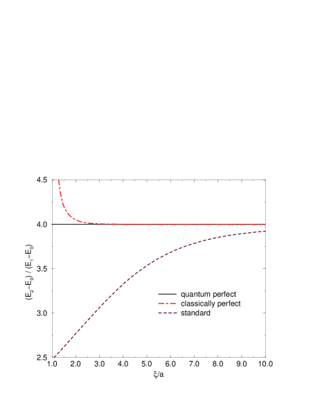
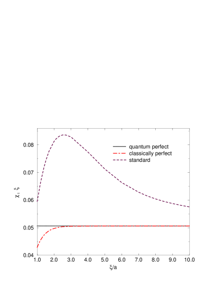
Figure 3: The scaling behaviour of a free scalar particle on a circle. We show two scaling quantities as functions of the correlation length in lattice units: the ratio between the first two energy gaps (on the left) and the topological susceptibility (on the right).

It is remarkable that also the continuum topology can be represented exactly on the lattice, thanks to the formulation with perfect actions and operators. Generally, we build (classically) perfect operators from the lattice fields obtained by (classical) blocking [15].

In contrast, for the standard action it is not even obvious how to define topological sectors (since all lattice configurations can be continuously deformed into one another). We use it here with the geometrical definition of the topological charge [17], which is the best option, but we observe strong scaling artifacts. On the other hand, the perfect formulation keeps track of each detail in the intervals between the discrete time points, since it emerges from blocking transformations. This means that any winding number between nearest neighbour time sites is included as a possibility in the expectation value $\langle\nu^{2}\rangle$. (Of course, a large number of windings is strongly suppressed by the kinetic term in the exponent of the Boltzmann factor, cf. eq. (1.13)). The classically perfect action still approximates the continuum value of $\,\chi_{t}\,\xi\,$ to a very good approximation.

3 Fermions

3.1 The Dirac equation

For convenience we temporarily return to Minkowski space for the Subsections 3.1 to 3.3, which contain introductory remarks on fermions.

Let us go back to quantum mechanics as a renewed starting point. Taking the relativistic energy-momentum relation $E^{2}=\vec{p}^{\,2}+m^{2}$ as a guide-line, one arrives at an obvious ansatz for a relativistic Schrödinger equation,

$$[\partial_{\mu}\partial^{\mu}-m^{2}]\,\Psi=0\ .$$ (3.1)

This is the Klein-Gordon equation, which we already encountered in eq. (1.8) in the context of classical field theory. An apparent problem with it, which worried the pioneers of quantum mechanics, is the occurrence of negative energies. P.A.M. Dirac wanted to avoid them by linearising this equation with the ansatz

$$[\,i\gamma_{\mu}\partial^{\mu}-m\,]\,\Psi=0\ .$$ (3.2)

In order to reproduce the relativistic energy, the coefficients $\gamma_{\mu}$ have to obey the anti-commutation relation

$$\{\gamma_{\mu},\gamma_{\nu}\}=2g_{\mu\nu}\ ,\quad g\equiv{\rm diag}(1,-1,-1,-1)\ .$$ (3.3)

Therefore, these coefficients $\gamma_{\mu}$ in the Dirac equation (3.2) have to be (at least) $4\times 4$ complex matrices in $d=4$. Thus the spinor $\Psi$ has four components,

$$\Psi=\left(\begin{array}[]{c}\psi_{1}\\ \psi_{2}\\ \psi_{3}\\ \psi_{4}\end{array}\right)\ .$$ (3.4)

Actually this linearisation does not overcome the negative energy eigenvalues. Nevertheless this ansatz was extremely successful; for instance, it led to the prediction of the positron just before its experimental discovery in 1931. In fact, the spinor $\Psi$ captures a spin-1/2 particle plus its antiparticle.

Later on, relativistic quantum mechanics considered the Dirac equation appropriate for fermions, and the Klein-Gordon equation for bosons.

3.2 Fermionic field theory

In the functional integral formulation of fermionic field theory, the Dirac operator is still present as the central ingredient in the Lagrangian. For free fermions of mass $m$, the partition function and the action are written as

$$Z = \int{\cal D}\bar{\Psi}{\cal D}\Psi\,e^{iS[\bar{\Psi},\Psi]}\ ,$$

$$S[\bar{\Psi},\Psi] = \int d^{4}x\,\bar{\Psi}(x)\,[i\gamma_{\mu}\partial^{\mu}-m]\,\Psi(x)\ ,$$ (3.5)

where $\bar{\Psi}(x)=(\bar{\psi}_{1}(x),\bar{\psi}_{2}(x),\bar{\psi}_{3}(x),\bar{\psi}_{4}(x))$ and $\Psi(x)$ are spinor fields. Application of the variational principle $\delta S=0$ leads to the Dirac equation (3.2) for $\Psi$, and to the adjoint Dirac equation

$$\bar{\Psi}\,[\,i\gamma_{\mu}\!\!\mathop{\raise 6.02773pt\hbox{$\leftarrow$\kern-7.5pt\raise-6.02773pt\hbox{$\partial$}}}\ ^{\!\!\mu}+m\,]=0\ .$$ (3.6)

In the light of the Spin-Statistics Theorem, fermion field components anti-commute, hence one describes them by Grassmann variables. A set of Grassmann variables $\{\eta_{i}\}$, $i=1,2,\dots$ (as it is used here for the components of $\bar{\Psi}$ and of $\Psi$ in a specific point $x$) obeys the relations

$$\{\eta_{i},\eta_{j}\}=0\ ,\quad\int d\eta_{i}\,\eta_{j}=\delta_{ij}\ .$$ (3.7)

A striking difference from the Dirac algebra (3.3) is the property $\eta_{i}^{2}=0$. The integration rule is motivated by the analogy to the translation invariance of the real, unbounded integral. The Grassmann integral has no bounds, and its effect is equivalent to differentiation. It provides the basis for the functional integral in eq. (3.5) [19], which we will make explicit in Subsection 3.4.

Interactions can be included for instance by adding a 4-Fermi term $(\bar{\Psi}(x)\,\Psi(x))^{2}$ to the Lagrangian, which we will consider in Subsections 3.5, 4.3 and 5.2. Another type of interaction is generated by coupling the fermions to a gauge field ${\cal A}_{\mu}$ through a covariant derivative, which turns the Dirac operator and the partition function into

$$D({\cal A}) = i\gamma_{\mu}\left[\partial^{\mu}-g{\cal A}^{\mu}(x)\right]-m\ ,$$ (3.8)

$$Z = \int{\cal D}\bar{\Psi}{\cal D}\Psi{\cal D}{\cal A}\,\exp\Big{(}i\int d^{4}x\,\bar{\Psi}(x)D({\cal A})\Psi(x)+iS[{\cal A}]\Big{)}\ .$$

$S[{\cal A}]$ represents the pure gauge action; it could be for instance the Abelian gauge action obtained by integrating the Lagrangian (1.9). In that framework, the term   $g\bar{\Psi}\gamma_{\mu}\Psi$   takes the rôle of the external, charged current $j_{\mu}$ (and $g$ is the gauge coupling). Fermionic $n$-point functions are defined in analogy to the bosonic case (see Subsection 1.3), but the order matters, of course.

3.3 Chiral symmetry

Due to the anti-commutation rule (3.3), the matrix

$$\gamma_{5}:=i\gamma_{0}\gamma_{1}\gamma_{2}\gamma_{3}\quad{\rm obeys}\quad\{\gamma_{5},\gamma_{\mu}\}=0\quad{\rm and}\quad\gamma_{5}^{2}=1\!\!1\ .$$ (3.9)

Therefore, the operators

$$P_{\pm}:=\frac{1}{2}(1\!\!1\pm\gamma_{5})$$ (3.10)

are complementary projectors ($P_{\pm}^{2}=P_{\pm}$ , $P_{+}+P_{-}=1\!\!1$). They can be used to decompose the spinor fields into their so-called left-handed and right-handed parts,

$$\Psi_{L,R}(x)=P_{\pm}\Psi(x)\ ,\quad\bar{\Psi}_{L,R}(x)=\bar{\Psi}(x)P_{\mp}\ .$$ (3.11)

In these terms, the fermionic part of the Lagrangian in eq. (3.8) reads

$${\cal L}=\bar{\Psi}_{L}D({\cal A})_{m=0}\Psi_{L}+\bar{\Psi}_{R}D({\cal A})_{m=0}\Psi_{R}-m(\bar{\Psi}_{L}\Psi_{R}+\bar{\Psi}_{R}\Psi_{L})\ .$$ (3.12)

In the chiral limit $m\to 0$ the left-handed and the right-handed parts decouple completely. This property corresponds to the relation

$$\{D_{m=0}\,,\gamma_{5}\}=0\ ,$$ (3.13)

which manifests itself in a global symmetry, namely the invariance of ${\cal L}$ under the “chiral rotation”

$$\bar{\Psi}\to\bar{\Psi}\,e^{i\alpha\gamma_{5}}\ ,\quad\Psi\to e^{i\alpha\gamma_{5}}\,\Psi\$$ (3.14)

for an arbitrary parameter $\alpha$.

Obviously, the term that enters the Lagrangian (3.12) for a fermion mass $m\neq 0$ breaks the chiral symmetry explicitly; the chiral rotation (3.14) transforms the mass term as

$$m\bar{\Psi}\Psi\ \to\ m\bar{\Psi}e^{2i\alpha\gamma_{5}}\Psi\ .$$ (3.15)

In general, global symmetries — such as the chiral invariance — are only realised approximately in Nature, hence a breaking by a mass term is not necessarily a problem. However, by the introduction of gauge fields one arrives at local symmetries, and they have got to be exact. In a vector theory, the gauge fields couple in the same way to the left-handed and to the right-handed fermions. This is the case for the gluon fields in QCD. Then the fermion mass is allowed — quark masses can be inserted into the QCD Lagrangian.

On the other hand, the electroweak sector of the Standard Model is an example for a chiral gauge theory, where the gauge fields couple in different ways to the left-handed and to the right-handed fermions. Then we have to require their invariance under independent transformations, which forbids explicit mass terms in ${\cal L}$. In that framework, the masses of fermions (and also those of gauge fields) can only be generated dynamically. It takes Yukawa couplings to a Higgs field and spontaneous symmetry breaking to arrive at massive quarks and leptons (and massive gauge bosons $W^{\pm}$ and $Z^{0}$).

3.4 Fermions on a Euclidean lattice

We return to Euclidean space, where the $\gamma$-matrices obey

$$\{\gamma_{\mu},\gamma_{\nu}\}=2\delta_{\mu\nu}\ ,\quad\gamma_{5}:=\gamma_{1}\gamma_{2}\gamma_{3}\gamma_{4}\ ,\quad\{\gamma_{\mu},\gamma_{5}\}=0\ ,\quad\gamma_{5}^{2}=1\!\!1\ .$$ (3.16)

We choose them to be Hermitian. We write a bilinear fermionic lattice action — such as the action for free fermions, or for fermions interacting through gauge fields — in the form

$$S=\sum_{i,j=1}^{N}{\bf\bar{\Psi}}_{i}M_{ij}{\bf\Psi}_{j}\equiv{\bf\bar{\Psi}}M{\bf\Psi}\ .$$ (3.17)

Here the components ${\bf\bar{\Psi}}_{i},\,{\bf\Psi}_{i}$ run over all the lattice sites, and on each site over all internal degrees of freedom (spinor and flavour indices, and for instance in QCD also colour indices). It is easy to see that the partition function is given by the celebrated fermion determinant,

$$Z=\int\prod_{i=1}^{N}d{\bf\bar{\Psi}}_{i}d{\bf\Psi}_{i}\ e^{-{\bf\bar{\Psi}}M{\bf\Psi}}={\rm det}M\ .$$ (3.18)

This expression also attaches an explicit meaning to the Grassmann functional integrals. (The order of the single Grassmann integrals matters, since the rule in eq. (3.7) refers particularly to the innermost integral.)

As an example, we consider a free, massless fermion with the Euclidean continuum action

$$S[\bar{\psi},\psi]=\int d^{4}x\,\bar{\psi}(x)\gamma_{\mu}\partial_{\mu}\psi(x)\ .$$ (3.19)

On a lattice with unit spacing ($a=1$) the simplest discretisation ansatz reads

$$S[\bar{\Psi},\Psi] = \sum_{x}\bar{\Psi}_{x}\gamma_{\mu}\frac{1}{2}(\Psi_{x+\hat{\mu}}-\Psi_{x-\hat{\mu}})$$ (3.20)

$$= \frac{1}{(2\pi)^{4}}\int_{B}d^{4}p\,\bar{\Psi}(-p)i\gamma_{\mu}\sin p_{\mu}\Psi(p)\ .$$

This formulation is known as the naive lattice fermion. As the name suggests, there is a serious problem with it: the propagator

$$G_{2}(p)_{\rm naive}=\frac{1}{i\gamma_{\mu}\sin p_{\mu}}$$ (3.21)

has inside the (first) Brillouin zone (2.1) not only the physical pole at $p=0$, but it has poles whenever $p_{\mu}\in\{0,\pi\}$, $\mu=1\dots 4$. Hence there are 16 poles (in general, $2^{d}$ poles) instead of the one that we have ordered. This effect is known as the fermion doubling problem — it is due to the occurrence of a linear derivative. In fact, these doublers distort physical properties regardless how fine the lattice might be, hence this formulation cannot be applied. For instance, among the 16 species the chiralities are equally distributed, which makes it impossible to construct a chiral gauge theory [22]. Moreover, the trouble also affects vector theories, since these species contribute to the axial anomaly with alternating signs, hence doubled lattice fermions cannot reproduce a non-vanishing axial anomaly either [23].

So we have to consider further options for the lattice action

$$S=\sum_{xy}\bar{\Psi}_{x}D_{xy}\Psi_{y}\ .$$ (3.22)

We recall that locality is in general a requirement for a controlled continuum limit (in view of the extension to the interacting case). In coordinate space, a local lattice Dirac operator $D$ has to be bounded as

$$|D_{xy}|\leq c_{1}e^{-c_{2}|x-y|}\quad,\qquad c_{1},\ c_{2}>0\ .$$ (3.23)

In momentum space this means that $D(p)=G_{2}(p)^{-1}$ has to be analytic.

It is not easy to find a satisfactory solution to the doubling problem. This statement was made precise by the Nielsen-Ninomiya No-Go Theorem [22]. Putting aside technical details, it essentially states that an undoubled lattice fermion cannot be chiral and local at the same time.

For an intuitive and simplified illustration, we write a rather general ansatz for a chiral lattice Dirac operator for free fermions,

$$D(p)=i\rho_{\mu}(p)\gamma_{\mu}\ ,\quad\rho_{\mu}(p)=p_{\mu}+O(p^{2})\ .$$ (3.24)

The leading momentum order of $\rho_{\mu}$ is required by the correct continuum limit (which is determined by small momenta in lattice units). We may consider the specific momenta $p=(p_{1},0,0,0)$, so that

$$D(p_{1},0,0,0)=i\rho_{1}(p_{1})\gamma_{1}\ ,$$

with the physical zero at $p_{1}=0$. Since $2\pi$ periodicity is mandatory, and since locality requires an analytic function $\rho_{1}(p_{1})=p_{1}+O(p_{1}^{2})$, at least one additional zero (generally: an odd number of them) is inevitable inside the Brillouin range $p_{1}\in\ (-\pi,\pi]$, even if one deviates from the naive form $\rho_{1}(p_{1})=\sin p_{1}$.

Many suggestions have been made to circumvent this problem by breaking one of the desired properties on the lattice, hoping this would not affect the continuum limit. We do not review all these efforts, but we mention as an example the SLAC fermion [24]. In the above consideration, it sets $\rho_{1}(p_{1})=p_{1}$ in $p_{1}\in\ (-\pi,\pi]$, which is then periodically continued (and the same for the other momentum components). Due to the jumps at the edges of the Brillouin zone this formulation is non-local. The hope to get away with this was crushed by Karsten and Smit, who showed that this formulation is inconsistent at the one-loop level of gauge theory, where it fails to reproduce Lorentz symmetry in the continuum limit [25].

The standard lattice fermion formulation, which has been used most in simulations — in QCD in particular — was put forward by K.G. Wilson in 1979 [27]. The free Wilson operator reads

$$D_{{\rm W},xy}=\frac{1}{2}\sum_{\mu}\Big{[}\gamma_{\mu}(\delta_{x,y-\hat{\mu}}-\delta_{x,y+\hat{\mu}})-(\delta_{x,y-\hat{\mu}}+\delta_{x,y+\hat{\mu}}-2\delta_{x,y})\Big{]}+m\delta_{x,y}\ .$$ (3.25)

Wilson added the term in the second round bracket to the naive form that we considered before. This term represents a Laplacian operator, which is discretised in the simplest way. In fact it avoids the fermion doubling by sending the doublers to the cutoff energy. There is no doubt that this operator is local, and the Wilson term is $O(a)$ suppressed, so one could hope that it does not distort the continuum limit.

However, due to this extra term the chiral symmetry is broken explicitly, $\{D_{{\rm W},m=0}\,,\gamma_{5}\}\neq 0$. As interactions are switched on, this causes numerous problems. In particular, a gauge field can be added as a set of link variables in the gauge group, which provides invariance under gauge transformation of the matter fields on the sites. One often writes this compact link variable as

$$U_{\mu,x}=\exp\Big{(}i\int_{x}^{x+\hat{\mu}}dy_{\mu}\,{\cal A}_{\mu}(y)\Big{)}\,\in\,{\rm\{\,gauge~{}group\,\}}\ ,$$ (3.26)

which indicates a connection to the (non-compact) continuum gauge field ${\cal A}_{\mu}$. For non-Abelian gauge groups this exponential is formulated as a path ordered product [28]. Such a gauge field suppresses the terms $\delta_{x,y\pm\mu}$ in the Wilson term, but not its last entry $2\delta_{x,y}$. This different treatment gives rise to additive mass renormalisation. If one tries to approach the chiral limit, where the renormalised fermion mass vanishes, one has to fine tune the bare mass to some value $m<0$, which compensates for the additive renormalisation.

A further (related) inconvenience for interacting Wilson fermions is that the lattice artifacts can appear in $O(a)$ already (unless one adds another term to cancel the $O(a)$ artifacts — following Symanzik’s program — which requires fine tuning again [29]).

Another formulation, which has been considered standard over the past decades, and which is regularly applied in simulations, is known as the staggered fermions (or Kogut-Susskind fermions) [30]. An elegant way to construct them starts from the naive action on a unit lattice,

$$S[\bar{\Psi},\Psi]=\sum_{x}\Big{[}\frac{1}{2}\sum_{\mu=1}^{d}\left(\bar{\Psi}_{x}\gamma_{\mu}U_{\mu,x}\Psi_{x+\hat{\mu}}-\bar{\Psi}_{x+\hat{\mu}}\gamma_{\mu}U_{\mu,x}^{\dagger}\Psi_{x}\right)+m\bar{\Psi}_{x}\Psi_{x}\Big{]}\ ,$$ (3.27)

and performs the substitutions [31]

$$\bar{\Psi}_{x}^{\prime}=\bar{\Psi}_{x}\gamma_{1}^{x_{1}}\dots\gamma_{d}^{x_{d}}\ ,\quad\Psi_{x}^{\prime}=\gamma_{d}^{x_{d}}\dots\gamma_{1}^{x_{1}}\Psi_{x}\ .$$ (3.28)

This leaves the mass term invariant and renders also the kinetic term diagonal in the spinor space. Hence one may reduce the transformed spinors to a single component $\bar{\chi}$, $\chi$, and one obtains

$$S[\bar{\chi},\chi] = \sum_{x}\Big{[}\frac{1}{2}\sum_{\mu=1}^{d}\Gamma_{\mu,x}\left(\bar{\chi}_{x}U_{\mu,x}\chi_{x+\hat{\mu}}-\bar{\chi}_{x+\hat{\mu}}U_{\mu,x}^{\dagger}\chi_{x}\right)+m\bar{\chi}_{x}\chi_{x}\Big{]}\ ,$$

$$\Gamma_{\mu,x} := (-1)^{x_{1}+x_{2}+\dots+x_{\mu-1}}\ .$$ (3.29)

This structure distinguishes two sublattices by the criterion if $\sum_{\mu=1}^{d}x_{\mu}$ is even or odd, i.e. by the sign term

$$\epsilon(x)=(-1)^{x_{1}+\dots+x_{d}}\ .$$ (3.30)

The link variables $U_{\mu,x}$ always connect sites belonging to distinct sublattices. For $m=0$, the action (3.29) is invariant under the transformations

$$\bar{\chi}_{x}\to e^{\alpha\epsilon(x)}\bar{\chi}_{x}\ ,\quad\chi_{x}\to e^{\alpha\epsilon(x)}\chi_{x}\ ,$$ (3.31)

which amounts to a remnant chiral symmetry $U(1)_{\rm e}\otimes U(1)_{\rm o}$, where $\epsilon(x)$ adopts the rôle of $\gamma_{5}$ (the subscripts refer to the even/odd sublattice). The $2^{d}$ components on the corners of the disjoint unit hypercubes are nowadays denotes as “tastes” (the earlier literature also called them “pseudoflavours”). As long as one finally assembles exactly 4 flavours from them, this remnant symmetry is sufficient to avoid additive mass renormalisation and $O(a)$ scaling artifacts.

Recently it became fashion to try to build single flavours with staggered fermions by taking the fourth root of the fermion determinant (3.18). However, it is likely that this formulation is non-local, and — even if someone is willing to accept that — additive mass renormalisation sets in again (see e.g. Refs. [32]). The question if this formulation might provide correct results even if it is non-local is still debated [33].

3.5 Are light fermions natural ?

We would like to stress that keeping track of the chiral symmetry is not a specific problem of the lattice regularisation. It should rather be viewed as a generic and deep problem, which plagues other regularisations as well. For instance, in dimensional regularisation [34] one performs computations in $4+\varepsilon$ dimensions (in the sense of distribution theory) and sends $\varepsilon\to 0$ at the end. This is the most popular regularisation scheme for perturbative calculations, but it is a longstanding problem to find a generally reliable rule for handling $\gamma_{5}=\prod_{\mu=1}^{d}\gamma_{\mu}$ on the regularised level (or $i\prod_{\mu=0}^{d-1}\gamma_{\mu}$ in the Minkowski signature), generalising eq. (3.16) (resp. (3.9)). A careful analysis of this issue can be found in Ref. [35].

On the conceptual level, this observation means that the existence of light fermions in our world actually appears to be unnatural. Nature must be non-perturbative, so we can only refer to a non-perturbative regularisation scheme when addressing this question, which means essentially the lattice. It is possible to formulate light lattice fermions — for instance light quarks in lattice QCD — but only with tedious and sophisticated constructions (see Section 7), which do not appear to mimic a conceivable mechanism in Nature. What could be an acceptable mimic is something very simple like the Wilson fermion (3.25), which, however, pushes the fermion mass to the cutoff scale due to a strong additive mass renormalisation — unless a negative bare mass is fine tuned, which appears unnatural again.

Nevertheless there do exist in particular two light quark flavours,

$$m_{u},\,m_{d}\ll\Lambda_{\rm QCD}\ .$$ (3.32)

The question how this is realised in Nature is a hierarchy problem that is not properly understood. The situation is different in pure Yang-Mills theory, for example, where (regularised) glueball masses can be made arbitrarily light thanks to asymptotic freedom and the absence of additive mass renormalisation. But for quarks it does not work in this simple way, due to the problems to keep track of an approximate chiral symmetry in a regularised system, such that the fermion mass is far below the cutoff. In a broader framework, this hierarchy problem raises the question why hadron masses are far below the Planck scale, and therefore why we do not just consist of gluons.

In Ref. [38] we studied the question if this problem could be solved (qualitatively) in a brane world. As a toy model, our target theory was the 2d Gross-Neveu model [39] with the (continuum) action

$$S[\bar{\Psi},\Psi]=\int d^{2}x\Big{[}\bar{\Psi}\gamma_{\mu}\partial_{\mu}\Psi-\frac{g}{2N}(\bar{\Psi}\Psi)^{2}\Big{]}\ ,$$ (3.33)

where we suppress the flavour index $1\dots N$. It enjoys a discrete chiral $Z(2)$ symmetry

$$(\bar{\Psi}_{L},\Psi_{L})\to\pm(\bar{\Psi}_{L},\Psi_{L})\ ,\quad(\bar{\Psi}_{R},\Psi_{R})\to\mp(\bar{\Psi}_{R},\Psi_{R})$$ (3.34)

(the chiral components are defined in eq. (3.11)). With an auxiliary scalar field $\Phi$ the action (3.33) is equivalent to

$$S[\bar{\Psi},\Psi,\Phi]=\int d^{2}x\Big{[}\bar{\Psi}\gamma_{\mu}\partial_{\mu}\Psi-\Phi\bar{\Psi}\Psi+\frac{N}{2g}\Phi^{2}\Big{]}\ ,$$ (3.35)

as we see by integrating out the field $\Phi$. The sign of $\Phi$ flips under a $Z(2)$ chiral transformation (3.34).

In the limit $N\to\infty$, $\Phi$ freezes to a constant [39], and $\bar{\Psi},\Psi$ can be integrated out. The resulting fermion determinant gives rise to an effective potential,

$$\int D\bar{\Psi}D\Psi\,e^{-S[\bar{\Psi},\Psi,\Phi]}=e^{-N\cdot V\cdot V_{\rm eff}(\Phi)}\ .$$ (3.36)

In a large volume $V$, the minima $\pm\Phi_{0}$ of $V_{\rm eff}$ obey the gap equation

$$\frac{1}{g}=\frac{1}{\pi}\int_{0}^{\Lambda_{2}}dk\,\frac{k}{k^{2}+\Phi_{0}^{2}}\quad\qquad(k=\sqrt{k_{1}^{2}+k_{2}^{2}})\ .$$ (3.37)

At weak coupling $g\ll 1$ we are dealing with a cutoff $\Lambda_{2}\gg\Phi_{0}$ and

$$m=\Phi_{0}=\Lambda_{2}\,e^{-\pi/g}$$ (3.38)

represents the fermion mass, which is generated by the spontaneous breaking of the $Z(2)$ symmetry (3.34). The exponent in eq. (3.38) expresses asymptotic freedom.

Let us proceed to three dimensions, where the action

$$S[\bar{\Psi},\Psi]\!=\!\!\int\!\!d^{3}x\Big{[}\bar{\Psi}\gamma_{\mu}\partial_{\mu}\Psi+\bar{\Psi}\gamma_{3}\partial_{3}\Psi-\frac{G}{2N}(\bar{\Psi}\Psi)^{2}\Big{]}\ ,\quad(\mu=1,2)$$ (3.39)

still has a $Z(2)$ symmetry,

$$(\bar{\Psi}_{L},\Psi_{L})|_{(\vec{x},x_{3})} \to \pm(\bar{\Psi}_{L},\Psi_{L})|_{(\vec{x},-x_{3})}\ ,$$

$$(\bar{\Psi}_{R},\Psi_{R})|_{(\vec{x},x_{3})} \to \mp(\bar{\Psi}_{R},\Psi_{R})|_{(\vec{x},-x_{3})}\ ,$$ (3.40)

which turns into the discrete chiral symmetry (3.34) after dimensional reduction. The 3d gap equation reads

$$\frac{1}{G}=\frac{1}{(2\pi)^{3}}\int d^{3}k\,\frac{2}{k^{2}+\Phi_{0}^{2}}\ ,$$ (3.41)

and for a cutoff $\Lambda_{3}\gg\Phi_{0}$ one identifies a critical coupling $G_{c}=\pi^{2}/\Lambda_{3}$. At $G>G_{c}$ we are in a phase of broken $Z(2)$ symmetry with

$$\Phi_{0}=2\pi\Big{(}\frac{1}{G_{c}}-\frac{1}{G}\Big{)}\ ,$$ (3.42)

whereas weak coupling ($G\leq G_{c}$) corresponds to a symmetric phase ($\Phi_{0}=0$).

Canonical dimensional reduction from 3 to 2 dimensions works in the usual way if we start from the 3d symmetric phase, and it leads to light 2d fermions [38]. However, this is not satisfactory in view of our motivation: for instance a non-perturbative treatment at finite $N$ (on the lattice) should not start from the symmetric phase, because this just shifts the problem of fine tuning to $d=3$. Therefore we focus on dimensional reduction from the broken phase.

We denote the (periodicity) extent of the third direction by $\beta$, and $\xi=1/m$ is the correlation length. Starting from the 3d broken phase, the limit  ${}^{\,\lim}_{\beta\to 0}\ \beta/\xi=2\ln(1+\sqrt{2})$ does not provide light fermions. Hence we proceed differently and generate a light 2d fermion as the $k_{3}=0$ mode on a brane. For the latter we make the ansatz $\Phi(x_{3})=\Phi_{0}\,{\rm tgh}(\Phi_{0}x_{3})$, which is inspired by Refs. [40]. We choose $x_{2}$ as the time direction, hence the Hamiltonian reads

$$\hat{H}=\gamma_{2}[\gamma_{1}\partial_{1}+\gamma_{3}\partial_{3}-\Phi(x_{3})]\ .$$ (3.43)

The ansatz $\Psi(x_{3})e^{ik_{1}x_{1}}e^{-iEt}$ (and the chiral representation for $\gamma_{i}$) reveals one localised eigenstate of $\hat{H}$,

$$\Psi_{0}(x_{3})=\sqrt{\frac{\Phi_{0}}{2}}\left(\begin{array}[]{c}0\\ \cosh^{-1}(\Phi_{0}x_{3})\end{array}\right)$$ (3.44)

with energy $E_{0}=-k_{1}>0$, i.e. a left-mover. (On an anti-brane $-\Phi(x_{3})$ one obtains a right-mover with $E_{0}=k_{1}>0$ and exchanged components in $\Psi_{0}(x_{3})$).

In addition there are bulk states (not localised in $x_{3}$),

$$\Psi_{k_{3}}(x_{3})=\frac{e^{ik_{3}x_{3}}}{\sqrt{2E(E+k_{1})}}\left(\!\!\begin{array}[]{c}i(E+k_{1})\\ \Phi_{0}{\rm tgh}(\Phi_{0}x_{3})-ik_{3}\end{array}\!\!\right)$$ (3.45)

with $E=\pm\sqrt{\vec{k}^{2}+\Phi_{0}^{2}}$, which form together with $\Psi_{0}$ an orthonormal basis for the 1-particle Hilbert space.

To verify the consistency of the brane profile we have to consider the chiral condensate $-\bar{\Psi}\Psi$. $\Psi_{0}$ does not contribute to it, and if we sum up the bulk contributions of $E<0$ we reproduce exactly $\Phi(x_{3})$, which confirms the self-consistency of this single brane world.

In addition we are free to fill some of the $\Psi_{0}$ states. Those with $E_{0}<\Phi_{0}$ are confined to the $(1+1)$-d world, whereas states with $E_{0}\geq\Phi_{0}$ can escape in the 3-direction. For the low energy observer on the brane this event appears as a fermion number violation.

We now want to include both, $\Psi_{L}$ and $\Psi_{R}$, to be localised on a brane and an anti-brane, and $\beta$ now denotes their separation. For the corresponding profile we make the ansatz

$$\Phi(x_{3}) = \Phi_{0}(a[{\rm tgh}_{+}-{\rm tgh}_{-}]-1)\ ,$$

$${\rm tgh}_{\pm} := {\rm tgh}(a\Phi_{0}[x_{3}\pm\beta/2])\ ,\ a\in[0,1]\ .$$ (3.46)

The ansatz for a bound state with the same form as on single branes,

$$\Psi_{0}(x_{3})=c\left(\begin{array}[]{c}\alpha_{1}\cosh^{-1}(a\Phi_{0}[x_{3}-\beta/2])\\ \alpha_{2}\cosh^{-1}(a\Phi_{0}[x_{3}+\beta/2])\end{array}\right),$$ (3.47)

implies the condition ${\rm tgh}(a\Phi_{0}\beta)=a$. Hence the parameter $a$ controls the brane separation, such that $a\to 0$ and $a\to 1$ correspond to $\beta\to 0$ and $\beta\to\infty$, respectively.

The Dirac equation in this background still has an analytic solution, which is given by the ansatz (3.47) with

$$c=\frac{1}{2}\sqrt{\frac{a\Phi_{0}}{E_{0}(E_{0}+k_{1})}}\ ,\ \ E_{0}=\pm\sqrt{k_{1}^{2}+m^{2}}\ ,$$

$$\alpha_{1}=-i(E_{0}+k_{1})\ ,\ \ \alpha_{2}=m=\sqrt{1-a^{2}}\,\Phi_{0}\ .$$ (3.48)

The resulting $\Psi_{0}(x_{3})$ represents a Dirac fermion with components $\Psi_{L}$, $\Psi_{R}$ localised on the brane resp. the anti-brane. For a fast motion to the left (right) we have $0<E_{0}\simeq-k_{1}\ (+k_{1})$, so that the lower (upper) component dominates. This situation is sketched in Figure 4. The mass $m$ measures the extent of the $L,R$ mixing. The limit $a\to 0$ does not provide a light fermion ($m=\Phi_{0}$), but the opposite limit $a\to 1$ achieves this, since the $L,R$ mixing is suppressed as

$$m\simeq 2\,\Phi_{0}\,e^{-\beta\Phi_{0}}\ .$$ (3.49)

Counter-intuitively, large $\beta$ implies $\xi\gg\beta$ and therefore dimensional reduction. A low energy observer in $d=1+1$ now perceives a point-like Dirac fermion composed of $L-$ and $R-$modes. On the other hand, a high energy observer in $d=2+1$ refers to the scale $\Phi_{0}$ (the 3d fermion mass) and observes a Dirac fermion with strongly separated $L-$ and $R-$constituents.

Also the bulk states can be determined analytically,

$$\Psi_{k_{3}}(x_{3}) = \frac{e^{ik_{3}x_{3}}}{\sqrt{U}}\left(\begin{array}[]{c}~{}~{}~{}i(E+k_{1})[a\Phi_{0}{\rm tgh}_{-}-ik_{3}]\\ -(\Phi_{0}+ik_{3})[a\Phi_{0}{\rm tgh}_{+}-ik_{3}]\end{array}\right)\ ,$$ (3.52)

$$U := 2E(E+k_{1})(k_{3}+a^{2}\Phi_{0}^{2})\ ,\ E=\pm\sqrt{k_{1}^{2}+k_{3}^{2}+\Phi_{0}^{2}}\ .$$

Summing up again their $E<0$ contributions to $-\bar{\Psi}\Psi$ yields

$$-\frac{G}{N}\int dk_{3}\Psi_{k_{3}}\bar{\Psi}_{k_{3}}\Big{|}_{E<0}=\Phi(x_{3})+{\cal C}\ ,$$ (3.53)

i.e. the desired result up to a term ${\cal C}$, which is given explicitly in Ref. [38]. It has to be cancelled by occupying bound states in $\Psi_{0}$, which do contribute this time. This requires all the bound states with energies $E_{0}\leq E_{F}$ to be filled. The Fermi energy turns out to be $E_{F}=\Phi_{0}$, i.e. exactly the threshold energy for the escape into the third dimension. Hence this brane anti-brane world does contain naturally light fermions, but it is completely packed with them, so its physics is blocked by Pauli’s principle.

Since this brane anti-brane world is not topologically stable, we also checked if the brane and anti-brane repel or attract each other, which could lead to disastrous scenarios. However, it turns out that the brane tension energy per fermion does not depend on the brane separation, so this toy world is indeed stable [38].

Finally we studied the possibility of adding a fermion mass term $M\bar{\Psi}\Psi$ to the Lagrangian, so that the $Z(2)$ symmetry is also explicitly broken in $d=3$ (which is actually realistic for a lattice formulation at finite $N$). This lifts the degeneracy of the minima of $V_{\rm eff}(\Phi)$. If we still insert the profile (3.46), the condition for $-\bar{\Psi}\Psi$ requires the bound fermion states to be filled even beyond $\Phi_{0}$, hence in this case there is no stable configuration at all.

One might also start from the symmetric phase and add a mass term to construct a somehow natural starting point. However, such a mass is simply inherited by the dimensionally reduced model (while the cutoff keeps the same magnitude), hence this does not solve the hierarchy problem under consideration.

We drop this mass term again and summarise Subsection 3.5 by repeating that the construction of naturally light fermions is basically successful, but unfortunately this world does not enjoy any flexibility for physical processes. However, we assumed translation invariance in the 2d world so far. That symmetry may be broken at sufficiently large chemical potential, so that the chiral condensate prefers a kink anti-kink pattern, rather than a constant [41]. This could possibly provide the missing flexibility for a lively brane world of that kind.

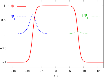
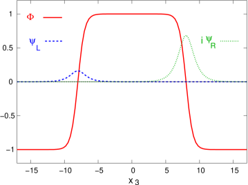
Figure 4: We show the brane anti-brane profile (3.46) in the 3-direction of our toy brane world [38]. The 2-direction is the (Euclidean) time, and the left-handed (right-handed) fermion moves to the left (right) in the one spatial direction inside the brane world. In the plot above it does so with a momentum $p_{1}=-4m$ and below with $p_{1}=2m$, where $m$ is the fermion mass. The latter arises from the communication between the left- and right-handed components, which are localised on the brane and anti-brane. As they drift apart, $m$ decreases exponentially in the distance, hence a low energy observer on the brane perceives them on top of each other as a point-like Dirac spinor.

4 Perfect Actions for Lattice Fermions

4.1 Free fermions

In the previous Section we have described the severe conceptual difficulties with the formulation of fermions on the lattice. We now proceed to the application of the RGT technique — described in Section 2 — to lattice fermions. This is going to reveal how the perfect action handles — and solves — the problems of species doubling and chiral symmetry.

We start with the free fermion and apply immediately the blocking from the continuum (introduced in Subsection 2.2), which is most efficient for analytic calculations. In analogy to eq. (2.10) we now relate lattice spinor fields $\bar{\Psi}_{x}$, $\Psi_{x}$ to their counterparts in the continuum,

$$\bar{\Psi}_{x}\sim\int_{C_{x}}d^{d}u\,\bar{\psi}(u)\ ,\quad\Psi_{x}\sim\int_{C_{x}}d^{d}v\,\psi(v)\ .$$ (4.1)

This relation is imposed by the RGT, which leads to the perfect lattice action $S[\bar{\Psi},\Psi]$ for free lattice fermions,

$$e^{-S[\bar{\Psi},\Psi]}=\int{\cal D}\bar{\psi}{\cal D}\psi\,e^{-s[\bar{\psi},\psi]}\times$$

$$\exp\Big{\{}-\sum_{xy}\Big{[}\bar{\Psi}_{x}^{i}-\int_{C_{x}}d^{d}u\,\bar{\psi}^{i}(u)\Big{]}(R^{-1})_{xy}^{ij}\Big{[}\Psi_{y}^{j}-\int_{C_{y}}d^{d}v\,\bar{\psi}^{j}(v)\Big{]}\Big{\}}\ ,\quad\$$ (4.2)

where $s[\bar{\psi},\psi]=\int d^{d}u\,\bar{\psi}(u)[\gamma_{\mu}\partial_{\mu}+m]\psi(u)$ is the continuum action (cf. eq. (3.19)). On the lattice (of spacing $a=1$) we arrive at the following perfect action and propagator

$$S[\bar{\Psi},\Psi] = \frac{1}{(2\pi)^{d}}\int_{B}d^{d}p\,\bar{\Psi}(-p)G(p)^{-1}\Psi(p)\ ,$$

$$G(p) = \sum_{l\in Z\!\!\!Z^{d}}\frac{\Pi(p+2\pi l)^{2}}{i\gamma_{\mu}(p_{\mu}+2\pi l_{\mu})+m}+R(p)\ ,$$ (4.3)

where the function $\Pi(p)$ is defined in eq. (2.11) (also here it could be generalised). This formula has been computed in various ways [42, 43, 15]. It incorporates the continuum propagator, its periodic copies and the blocking term, in full analogy to the perfect action for free scalars in eq. (2.11).

Let us now discuss the rôle of the blocking term, which we have generalised from the constant $1/\alpha$ in the scalar case (eq. (2.5)) to the form $R_{xy}^{ij}$. For sure we have to require $R$ to be local. Thus it cannot disturb the pole structure of $G(p)$. Hence the formulation is free of doublers, and the dispersion relation coincides with the continuum.

In the limit $R\to 0$ we perform a $\delta$-function blocking, as we mentioned for the scalar fields before. Then the relations (4.1) turn into equations. In this case (or more generally, whenever $\{R,\gamma_{5}\}$ vanishes), $G(p)_{m=0}$ — and therefore also the Dirac operator $D(p)_{m=0}$ — anti-commutes exactly with $\gamma_{5}$. Then we have chirality, i.e. invariance under the global transformation (3.14), just as in the continuum. Hence the question arises in which way a contradiction to the (mathematically rigorous) Nielsen-Ninomiya Theorem [22] is avoided. The answer is that in this case the Dirac operator is non-local [42, 43]: it does not decay exponentially, but only as [15]

$$D(r)_{m=0}\propto\frac{1}{r^{d-1}}\ .$$ (4.4)

As soon as we proceed to some non-vanishing, local term $R$, which obeys

$$\{R,\gamma_{5}\}\neq 0\ ,$$ (4.5)

locality is restored. However, this obviously leads to

$$\{D(p)_{m=0},\gamma_{5}\}\neq 0\ ,$$ (4.6)

hence we do not have chirality in the standard form (3.14) anymore.

Still, this breaking of the chiral symmetry can only be superficial: we know that the RGT does not distort any physical properties, hence the chirality of the continuum must be preserved in the physical observables, despite the relation (4.6), as we emphasised at numerous occasions [46, 47, 15, 48]. Therefore this must be a specifically harmless anti-commutator. Indeed it gave the crucial clue for a general criterion for the form of such a non-vanishing anti-commutator [45], which is still compatible with chiral symmetry in a lattice modified form [49]. This criterion is now denoted as the Ginsparg-Wilson relation (since it was already mentioned in Ref. [44]), which we will discuss in Section 7.

We assume $R$ to have the structure of a Dirac scalar, and we move to coordinate space. The perfect action for the free fermion is given in the form

$$S[\bar{\Psi},\Psi] = \sum_{x,y}\bar{\Psi}_{x}D_{xy}\Psi_{y}\ ,$$

$$D_{xy} = (G^{-1})_{xy}=\gamma_{\mu}\rho_{\mu}(x-y)+\lambda(x-y)\ ,$$ (4.7)

i.e. it consists of a vector term plus a scalar term. We consider the local case (4.5), where $\rho_{\mu}(x-y)$ and $\lambda(x-y)$ decay exponentially in the distance $|x-y|$. For practical purposes we need a truncation in these couplings, and we follow again the scheme of Section 2: we first optimise $R$, for the case $R_{xy}^{ij}=\rho\,\delta_{xy}\delta^{ij}$. An analytic calculation in $d=1$ suggests the choice

$$\rho(m)=\frac{e^{m}-m-1}{m^{2}}\ .$$ (4.8)

Only for this form of $\rho(m)$ the 1d couplings are limited to nearest neighbour sites, i.e. they take the structure of $D_{\rm W}$. In $d\geq 2$ couplings over all distances are inevitable, but the choice (4.8) still provides practically optimal locality, i.e. optimally fast exponential decays of the functions $\rho_{\mu}(x-y)$ and $\lambda(x-y)$; this is illustrated in Ref. [15].

As a truncation scheme, we computed for this function $\rho(m)$ the couplings of perfect actions in a periodic $3^{4}$ lattice, and applied these couplings in larger volumes [50]. This yields the free hypercube fermion (HF), which still has the structure of eq. (4.7), but now with strictly limited supports for the ingredients to the Dirac operator,

$$D_{{\rm HF},xy}=\gamma_{\mu}\rho_{\mu}(x-y)+\lambda(x-y)\ ,$$

$${\rm supp}[\rho_{\mu}(x-y)],\ {\rm supp}[\lambda(x-y)]\subset\Big{\{}x,y\ \Big{|}\ |x_{\mu}-y_{\mu}|\leq 1\ ,\ \forall\mu\Big{\}}\ .\quad$$ (4.9)

Tables for the explicit couplings for such HFs at various masses are given in Ref. [50]; in Table 1 we display here the HF couplings at $m=0$ to an extended precision of 16 digits.

$r$	$\rho_{1}(r)$	$\lambda(r)$
$(0,0,0,0)$	0	$1.852720547165511$
$(1,0,0,0)$	$0.1368467943177540$	$-0.060757866428667176$
$(1,1,0,0)$	$0.032077284302446526$	$-0.030036032105554878$
$(1,1,1,0)$	$0.011058131255574036$	$-0.015967620416694967$
$(1,1,1,1)$	$0.0047489906005042248$	$-0.0084268119917885868$

Table 1: The couplings of the free, massless HF with the parameterisation of eq. (4.9). $\rho_{\mu}(r)$ is anti-symmetric in $r_{\mu}$ and symmetric in all other components $r_{\nu}$, while $\lambda(r)$ is symmetric in all directions.

After truncation, the scaling behaviour is still by far superior to the Wilson fermion, and also to the so-called D234 fermion [51], which is improved to the leading order in the lattice spacing, following Symanzik’s program. A comparison of the dispersion relations at mass $m=0$ and $1$ is shown in Figure 5. We see a striking improvement for the truncated perfect action.

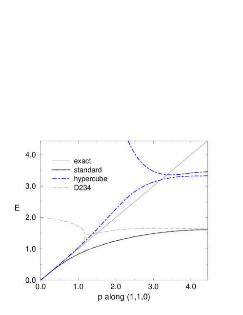
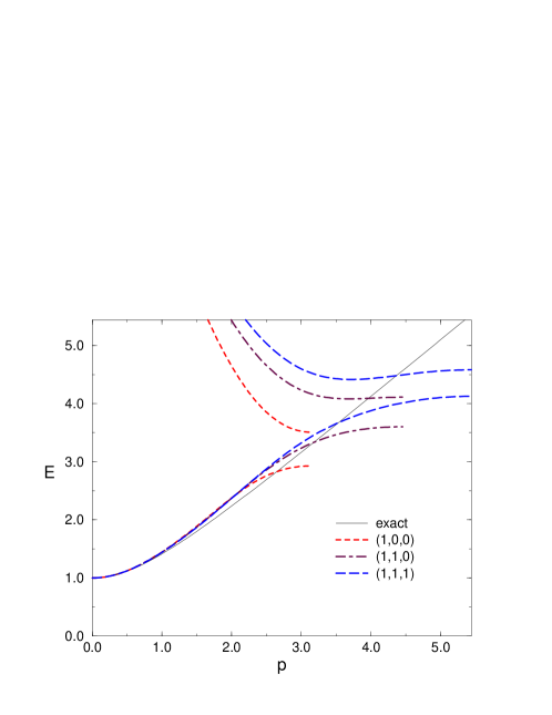
Figure 5: On top: The dispersion relation for free, massless lattice fermions in $d=4$ for spatial momenta $\vec{p}\propto(1,1,0)$ (as an example). For the perfect fermion the dispersion coincides with the exact dispersion in the continuum, and the HF dispersion follows it closely. The standard Wilson fermion deviates strongly at increasing momenta, while the Symanzik improved D234 fermion behaves well up to $|\vec{p}\,|\approx 1$, before it hits a doubler coming down from higher energy.
Below: Dispersion relation for the free HF at mass $m=1$. Here we show the energy $E$ for various directions of the momentum $\vec{p}$ ($p=|\vec{p}\,|$) to illustrate that they all follow closely the continuum dispersion over a sizable part of the Brillouin zone.

This trend is also confirmed for the thermodynamic quantities plotted in Figures 6 and 7. The pressure $P$ at finite temperature $T$ is obtained by imposing periodic boundary conditions in the time direction over $N_{t}$ lattice points. The corresponding data in Figure 6 are evaluated with the formula

$$\frac{P}{T^{4}} = \frac{N_{t}^{4}}{(2\pi)^{3}}\int_{-\pi}^{\pi}d^{3}p\,\Big{[}\frac{1}{N_{t}}\sum_{n=1}^{N_{t}}\ln{\rm det}D(\vec{p},p_{4,n})\Big{|}_{p_{4,n}=2\pi(n-1/2)/N_{t}}$$ (4.10)

$$\hskip 79.6678pt-\frac{1}{2\pi}\int_{-\pi}^{\pi}dp_{4}\,\ln{\rm det}D(\vec{p},p_{4})\Big{]}\ .$$

In this case we find a deviation from the continuum value $P/T^{4}=7\pi^{2}/180$ even for the perfect action, because its perfection is designed specifically for zero temperature.

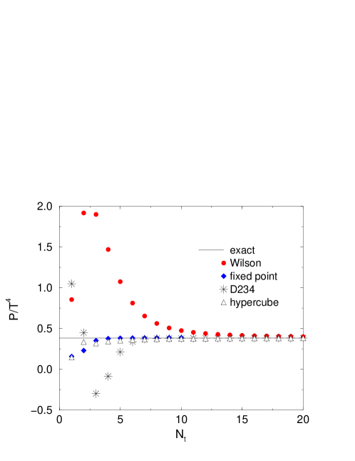
Figure 6: The ratio between ${\rm pressure}$ and ${\rm(temperature)}^{4}$ for various types of free lattice fermions, compared to the Stefan-Boltzmann law in the continuum. The RGT improved actions converge much faster to this value for decreasing temperature (increasing $N_{t}$) than the Wilson action or the D234 action.

Figure 7 deals with the inclusion of the chemical potential $\mu$. This is achieved by the prescription worked out in Refs. [52]. The key observation is that starting from any prefect lattice action at $\mu=0$ and performing consistently the substitutions

$$\bar{\Psi}(\vec{x},x_{4})\to e^{-\mu x_{4}}\bar{\Psi}(\vec{x},x_{4})\ ,\quad\Psi(\vec{x},x_{4})\to e^{\mu x_{4}}\Psi(\vec{x},x_{4})\ ,$$ (4.11)

one obtains in fact a perfect action at finite $\mu$. (Also classical perfection is preserved under these substitutions.) In our perfect propagator in momentum space (4.3), this substitution can be implemented by shifting $p_{4}\to p_{4}+i\mu$. Then one obtains the pressure and the baryon density (one third of the fermion density) at $T=0$ as

$$P(\mu) = \frac{1}{(2\pi)^{4}}\int_{B}d^{4}p\,\Big{[}\ln{\rm det}D(\vec{p},p_{4})-\ln{\rm det}D(\vec{p},p_{4}+i\mu)\Big{]}\ ,$$

$$n_{B} = \frac{1}{3}\frac{\partial}{\partial\mu}P(\mu)\ .$$ (4.12)

The scaling is then measured by the deviations from the continuum values $P/\mu^{4}=1/(6\pi^{2})$ and $n_{B}/\mu^{3}=2/(9\pi^{2})$. Lattice artifacts are amplified for increasing chemical potential $\mu$. We see that they remain modest over a broad range (i.e. up to coarse lattices) for the truncated perfect action, in contrast to the Wilson fermion and the D234 fermion. For large $\mu$ the fermion density turns into a constant plateau for the usual lattice fermion formulations, and one might believe that this is inevitable due to Pauli’s principle. However, the height of this plateau depends on the coupling range of the lattice Dirac operator, and it rises to infinity for the (untruncated) perfect action — hence the RGT is able to solve this problem as well [52].

Figure 7: The ratios $P/\mu^{4}$ and $n_{B}/\mu^{3}$, for the pressure $P$, the baryon density $n_{B}$ and the chemical potential $\mu$, at zero temperature, for various types of free massless lattice fermions. For the truncated perfect HF these ratios converge very fast to the continuum values as $\mu$ decreases, in contrast to the Wilson fermion and the D234 fermion.

4.2 Perfect staggered fermions

As we pointed out in the previous Subsection, the full standard chiral symmetry cannot be preserved in a perfect and local lattice action. On the other hand, staggered fermions only have a remnant chiral symmetry — see Subsection 3.4 — which raises the question if that symmetry can persist in a perfect and local staggered fermion formulation. In fact, this $U(1)_{\rm o}\otimes U(1)_{\rm e}$ symmetry can be preserved under the RGT, if the block variables are constructed such that they do not mix any of the $2^{d}$ tastes. A corresponding blocking scheme with overlapping blocks was first proposed in Ref. [53]. By its iteration we constructed a perfect action for free staggered fermions [43], which does fulfil the $U(1)_{\rm o}\otimes U(1)_{\rm e}$ symmetry exactly, and which is manifestly local — the Nielsen Ninomiya Theorem does not exclude this remnant chiral symmetry. In $d=2$ the corresponding free perfect action for the four massless tastes reads

$$S[\bar{\chi},\chi] = \sum_{x,y}\sum_{i,j=1}^{4}\bar{\chi}^{i}_{x}[\alpha^{-1}]^{ij}(x-y)\chi^{j}_{y}\ ,$$ (4.13)

$$\tilde{\alpha}(p) = d(-p)\alpha(p)d(p)=\left(\begin{array}[]{cccc}0&\tilde{\alpha}_{1}(p)&\tilde{\alpha}_{2}(p)&0\\ \tilde{\alpha}_{1}(p)&0&0&-\tilde{\alpha}_{2}(p)\\ \tilde{\alpha}_{2}(p)&0&0&~{}~{}~{}\tilde{\alpha}_{1}(p)\\ 0&\tilde{\alpha}_{1}(p)&\tilde{\alpha}_{2}(p)&0\end{array}\right)$$ (4.18)

$$\tilde{\alpha}_{\mu}(p) = 2\sum_{l\in Z\!\!\!Z^{2}}\frac{p_{\mu}+2\pi l_{\mu}}{(p+2\pi l)^{2}}(-1)^{l_{\mu}}\,\prod_{\nu=1}^{2}\Big{(}\frac{\sin(p_{\nu}/2)}{p_{\nu}/2+\pi l_{\nu}}\Big{)}^{2}+c\sin(k_{\mu}/2)\ ,$$

where $d(p)$ is a matrix of phase factors, which arrange for the shifts to the appropriate lattice sites (it is given explicitly in Ref. [56], which denotes it as $D(p)^{1/2}$). $c$ is an arbitrary (real) RGT parameter, which we tuned again for optimal locality. In this case, the analytic optimisation in $d=1$ yields $c=1/2$. Ref. [57] discusses the extension of this action to $d=4$, as well as the generalisation to a finite fermion mass $m$, which fills in diagonal elements in the above matrix and changes the locality optimal RGT term.

Also this result can be derived efficiently by blocking from the continuum, if the overlapping integration cells are treated carefully. That method also allows for a blocking of non-compact gauge fields, which is consistent in the sense that the link variables never connect fermionic variables on the same sublattice [57].

4.3 Application to the Gross-Neveu model

We return to the Gross-Neveu model that we described previously in Subsection 3.5. More precisely we now consider its lattice formulation in terms of staggered fermions. Again we replace the 4-Fermi term by a Yukawa coupling to an auxiliary scalar field $\phi$. Since $\phi$ is taste-free, it is adequate to put its lattice variables on the cell centres $z$ of the fermionic lattice [58]. The standard formulation then couples $\phi_{z}$ in the same manner to the $2^{d}$ taste variables located on the corners of the cell with centre $z$.

As in Subsection 3.5 we considered the large $N$ limit, where the field $\phi_{z}$ freezes to a constant $\phi^{(0)}$. Then the fermions can be integrated out, so that the RGT can be computed explicitly. In Ref. [56] we derived the perfect staggered fermion action for this case. To analyse the scaling behaviour, we evaluated two quantities of dimension mass for the staggered standard action and for the perfect action:

• First we computed the chiral condensate $\langle\chi\bar{\chi}\rangle$. For the perfect action $S[\bar{\chi},\chi,\phi]$ this was achieved by a perturbation

  $$S_{\epsilon}[\bar{\chi},\chi,\phi]=S[\bar{\chi},\chi,\phi]+\epsilon X[\bar{\chi},\chi,\phi]\ .$$ (4.19)

  The operator $X$ has the standard lattice form $\sum_{x}\chi_{x}\bar{\chi}_{x}$, and its perfect lattice form was computed again by the RGT technique, i.e. this perturbation was included to $O(\epsilon)$ in the transformation.

• From the gap equation (analogous to the continuum eq. (3.37))

  $$2\phi^{(0)}=\frac{g}{(2\pi)^{2}}\int_{B}d^{2}p\,\ln\,{\rm det}M(p,\phi^{(0)})$$ (4.20)

  we extracted the fermion mass $m_{f}$, which is dynamically generated by the breaking of the discrete, remnant chiral symmetry. $M$ is the fermion determinant (see eq. (3.18)), either for the standard formulation or for the perfect formulation.

  In this context, we also considered the asymptotic scaling by investigating how closely $\phi^{(0)}(1/g)$ follows an exponential behaviour. (This behaviour is known in the continuum version of this model, see eq. (3.38), and it characterises asymptotic freedom.) Theoretically, asymptotic scaling does not need to be improved by the perfect action, since it is in principle independent from the scaling itself. Nevertheless we observed that it is significantly improved as well [56], in agreement with similar observations for truncated classically perfect actions for $SU(3)$ gauge theory [59].

While these calculations involve lengthy expressions, the outcome for the (dimensionless) ratio of these two terms, which represents our scaling quantity, takes a simple form,

$$\frac{\langle\chi\bar{\chi}\rangle}{m_{f}}\Big{|}_{\rm standard}=\frac{2\sinh(am_{f}/2)}{am_{f}}\quad,\qquad\frac{\langle\chi\bar{\chi}\rangle}{m_{f}}\Big{|}_{\rm perfect}=1\ .$$ (4.21)

Hence the perfect scaling is indeed confirmed, i.e. for the perfect action the considered scaling ratio takes the exact continuum value at any lattice spacing $a$. In contrast, for the standard action this ratio is only obtained in the limit $a\to 0$. We add that in this case also the classically perfect action scales perfectly; artifacts are switched off by the large $N$ limit [56].

4.4 Exact supersymmetry on the lattice

Since the RGT technique enables us to transfer continuum properties to the lattice without any damage in the physical observables, this procedure can in principle also preserve exact supersymmetry (SUSY) on the lattice [60]. This may appear surprising, because continuous SUSY seems to contradict the lattice structure. For a review which presents a variety of approaches to handle SUSY on the lattice we refer to Ref. [61], and examples for further efforts to construct exact lattice SUSY are collected in Refs. [62].

For an illustration of the perfect action treatment of SUSY, we considered the simplest supersymmetric model [63]: it is given in $d=2$ by the Lagrangian

$${\cal L}[\psi,\varphi]=\bar{\psi}\gamma_{\mu}\partial_{\mu}\psi+\partial_{\mu}\varphi\partial_{\mu}\varphi\ ,$$ (4.22)

with a Majorana spinor $\psi$ and a neutral scalar field $\varphi$. The action is invariant under simultaneous transformations with

$$\delta\psi=-\gamma_{\mu}\partial_{\mu}\varphi\,\varepsilon\ ,\quad\delta\varphi=\bar{\varepsilon}\,\psi\ ,$$ (4.23)

where $\varepsilon$ is a two-component Grassmann vector. The SUSY transformation generators form a closed algebra with the translation operators,

$$[\delta_{1},\delta_{2}]\varphi=(\bar{\varepsilon}_{1}\gamma_{\mu}\varepsilon_{2}-\bar{\varepsilon}_{2}\gamma_{\mu}\varepsilon_{1})\partial_{\mu}\varphi\ .$$ (4.24)

By blocking from the continuum we transfer this model to the unit lattice and arrive at

$$S[\Psi,\Phi] = \frac{1}{(2\pi)^{2}}\int_{B}d^{2}p\,\Big{[}\bar{\Psi}(-p)G(p)^{-1}\Psi(p)+\Phi(-p)G_{s}(p)^{-1}\Phi(p)\Big{]}\ ,$$

$$G_{s}(p) = \sum_{l\in Z\!\!\!Z^{2}}\frac{\Pi(p+2\pi l)^{2}}{(p_{\mu}+2\pi l_{\mu})^{2}}+R^{s}(p)\ ,$$ (4.25)

where $G$ is the perfect fermion propagator (4.3), and $G_{s}$ is a perfect scalar propagator (an obvious generalisation of the form given in eq. (2.11)). If we perform the SUSY transformations (4.23) in the continuum, they are carried over to the blocked lattice fields,

$$\delta\Psi_{x}=-\gamma_{\mu}\int_{C_{x}}\partial_{\mu}\varphi(u)du\ \varepsilon\ ,\quad\delta\Phi_{x}=\bar{\varepsilon}\int_{C_{x}}\psi(u)du\ ,$$ (4.26)

which — under these transformations — obey exact SUSY too.

In particular, we may treat the term $j_{\mu}=\gamma_{\mu}\varphi$ as a continuum current. As a general prescription we block a continuum current to the lattice by integrating its flux over the face $f_{\mu,x}$ between adjacent lattice cells [46],

$$J_{\mu,x}=\int_{f_{\mu,x}}d^{d-1}y\,j_{\mu}(y)\ .$$ (4.27)

This blocking scheme is illustrated in Figure 8 on the right-hand side. The lattice divergence of the blocked current is then equal to the continuum divergence integrated over the corresponding lattice cells,

$$\delta J_{x}=\sum_{\mu}(J_{\mu,x+\hat{\mu}/2}-J_{\mu,x-\hat{\mu}/2})=\int_{C_{x}}d^{d}y\,\partial_{\mu}j_{\mu}(y)\ .$$ (4.28)

In this way, the transformations (4.26) can be expressed solely in terms of lattice quantities, i.e. the lattice current and the blocked lattice field [60]. Accordingly, the algebraic relation (4.24) is now precisely reflected in terms of lattice quantities as

$$[\delta_{1},\delta_{2}]\Phi=(\bar{\varepsilon}_{1}\nabla_{\mu}J_{\mu}\varepsilon_{2}-\bar{\varepsilon}_{2}\nabla_{\mu}J_{\mu}\varepsilon_{1})\ ,$$ (4.29)

where $\nabla_{\mu}$ is the standard (symmetric) lattice derivative.

These properties also extend to the free 2d Wess-Zumino model, which involves an additional scalar field that balances the fermionic and bosonic degrees of freedom, and to the free 4d Wess-Zumino model, where further field components are added.

In terms of classically perfect fields, the continuum SUSY transformations can be carried over to the lattice also in the interacting case. However, the explicit construction of the corresponding lattice terms is a challenging numerical project, which has not been carried out so far.

Still the lattice is hostile by its nature towards SUSY. In order to simulate SUSY models nevertheless, also the discrete formulation on a fuzzy sphere — that we already mentioned in Subsection 3.5 — should be considered [64]. For corresponding simulations we refer to Refs. [65, 66].

Figure 8: A cartoon of the schemes that we used to block various quantities from the continuum: matter fields are blocked to the lattice by integrating the continuum field in a lattice cell, with the convolution function $\Pi$. The perfect propagator $G$ is obtained by integrating all continuum propagators between points in the corresponding lattice cells, as shown on the left (the formulae are given in Subsections 2.2, 4.1 and 4.2). In the centre we illustrate the blocking for gauge fields, to be discussed in detail in Subsection 5.3. Here we integrate all straight parallel transporters between continuum points, which have the same relative position in adjacent lattice cells. At last, a perfect current is obtained by integrating the continuum flux through the face between adjacent lattice cells (it will be used again Subsection 5.3).

5 Perfect Lattice Perturbation Theory

On the level of analytical calculations, the construction of perfect lattice actions can be extended from the free fields to perturbative interactions. As a first example, we already sketched the computation of a perfect chiral condensate in Subsection 4.3.

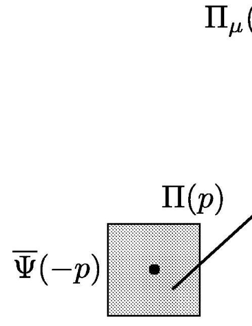
Figure 10: Overview over the construction scheme of the perfect quark gluon vertex function: the lattice fermion fields $\bar{\Psi}$ and $\Psi$ and the gluon field $A_{\mu}$ are obtained by blocking from the continuum, cf. Figure 8. For a given point (as the one marked by the central dot in this Figure) we then integrate the continuum propagators to all continuum fields involved in this blocking process.

The method of blocking from the continuum is still applicable and highly efficient for this purpose. One now blocks various fields in such a way that all the continuum propagators between the continuum points in the lattice cells are integrated over. In the case of gauge interactions, also the gauge fields undergo a blocking procedure, which can be made explicit most conveniently for non-compact gauge fields, see Subsections 5.3 and 5.4, and for illustrations Figures 8 and 10.

5.1 The anharmonic oscillator

As a toy model from quantum mechanics, we considered the anharmonic oscillator [67]. We write its action in field theoretic notation as

$$s[\varphi]=\int dt\,\Big{[}\,\frac{1}{2}\dot{\varphi}(t)^{2}+\frac{m^{2}}{2}\varphi(t)^{2}+\lambda\varphi(t)^{4}\,\Big{]}\ ,\quad(\varphi(t)\in{\kern 2.5pt\sf{R}\kern-7.79999pt\sf{I}\kern 7.79999pt\kern-2.5pt})\ .$$ (5.1)

As in the case of the quantum rotor (discussed in Refs. [16, 18] and reviewed in Subsection 2.3), we use the ratio between the first two energy gaps, $\Delta E_{1}=E_{1}-E_{0}$ and $\Delta E_{2}=E_{2}-E_{0}$, as a scaling quantity. In continuum perturbation theory, the corresponding expansion can be found at many places in the literature, e.g. in Ref. [68]. In terms of the dimensionless interaction parameter $\bar{\lambda}:=\lambda/m^{3}$ one obtains

$$\frac{\Delta E_{2}}{\Delta E_{1}}(\bar{\lambda})=2+3\bar{\lambda}-\frac{189}{4}\bar{\lambda}^{2}+\frac{7857}{8}\bar{\lambda}^{3}-\frac{1569069}{64}\bar{\lambda}^{4}+O(\bar{\lambda}^{5})\ .$$ (5.2)

First we evaluated this ratio to a high precision by Metropolis Monte Carlo simulations and we compare it to the perturbative results in various orders in Figure 9 (above). The latter approach the correct result only laboriously in a small range for $\bar{\lambda}$, even if we include the fourth order. This may serve as a caution to be careful in general with extrapolations to finite interaction strength based on perturbation theory.

Figure 9: Above: The ratio between the leading energy gaps, $\Delta E_{2}/\Delta E_{1}$, against the perturbative predictions. Higher orders do extend the range of the validity of perturbation theory gradually, but even at fourth order it is still limited to small interaction parameters ($\bar{\lambda}\mathop{\raise 1.29167pt\hbox{$<$\kern-7.5pt\raise-4.73611pt\hbox{$\sim$}}}0.03$).
In the plot below we compare simulation results at $\bar{\lambda}=0.005$ with the standard action and the $O(\bar{\lambda})$ perfect action, for different correlation lengths $\xi$ in lattice units [67].

Next we calculated the perfect lattice action to $O(\bar{\lambda})$. We chose the RGT parameter so that the action at $\bar{\lambda}=0$ consists of nearest neighbour couplings only. This is possible in 1d field theory (i.e. quantum mechanics) with the parameter given in eq. (2.13). We then extended the blocking from the continuum to $O(\bar{\lambda})$. This generates additional 2-spin and 4-spin terms, which were written down explicitly in momentum space [67]. There inverse Fourier transform yields a set of couplings that we computed for various parameters $m^{2}$ up to a coupling distance of two lattice spacings. This truncation is justified because the couplings undergo a fast decay, which speeds up for increasing $m^{2}$.

Finally we simulated the resulting perturbatively perfect action. For the scaling test, we fixed $\bar{\lambda}=0.005$, i.e. a value where Figure 9 (above) suggests the validity of first order perturbation theory. The results at various correlation lengths are compared to the outcome with the standard action in Figure 9 (below). At a correlation length of $\xi=5$ (in lattice units), both actions perform very well, and below 2.5 both suffer from similar scaling artifacts. In between, there appears a window where the perturbatively perfect action seems superior, as we observed at $\xi=10/3$.

5.2 The Yukawa term

We computed a perturbatively perfect action in the framework of the Gross-Neveu model with staggered fermions, cf. Subsections 4.2 and 4.3, but now for four tastes. In this case (without a large $N$ limit), the auxiliary scalar field $\Phi$ is not constant anymore, but we assumed it to be small. More precisely, we absorbed the Yukawa coupling in $\Phi$ and considered its first order. In this approximation — which describes the asymptotically free system at high energy — the perfect staggered action takes the form

$$S[\bar{\chi},\chi,\Phi] = \sum_{xy,ij}\bar{\chi}_{x}^{i}[\alpha^{-1}]_{xy}^{ij}\chi_{y}^{j}+\frac{1}{2}\sum_{z}\Phi_{z}^{2}$$ (5.3)

$$+ \sum_{xyz,ij}\bar{\chi}_{x}^{i}\sigma^{ij}(x-z,y-z)\chi^{j}_{y}\Phi_{z}\ ,$$

where $x,y$ run over the lattice which hosts the fermionic degrees of freedom, whereas $z$ runs over the plaquette centres, and $i,j=1\dots 4$. If we take the spacing between fermion components of the same taste as the unit, $z$ is spaced by $1/2$. In momentum space we write the interaction term as $\bar{\chi}(-p)\sigma(p,q)\chi(-q)\Phi(p+q)$. In the taste space, the shifted kernel $\tilde{\sigma}$ is a $4\times 4$ matrix, which only couples tastes of the same sublattice. To be explicit, its first order perturbatively perfect form reads [56] (we use the notation of eq. (4.13))

$$\tilde{\sigma}(p,q)=d(p)\alpha(p)\sigma(p,q)\alpha(-q)d(-q)=\left(\begin{array}[]{cccc}\tilde{\sigma}_{0}&0&0&-\tilde{\sigma}_{3}\\ 0&\tilde{\sigma}_{0}&\tilde{\sigma}_{3}&0\\ 0&-\tilde{\sigma}_{3}&\tilde{\sigma}_{0}&0\\ \tilde{\sigma}_{3}&0&0&-\tilde{\sigma}_{0}\end{array}\right)\ ,$$ (5.4)

with the matrix elements

$$\tilde{\sigma}_{0}(p,q) = \sum_{l,m\in Z\!\!\!Z^{2}}\sum_{n}\frac{p_{\mu}^{(l,n)}q_{\mu}^{(m,n)}}{p^{(l,n)\,2}q^{(m,n)\,2}}$$

$$\times \prod_{\nu=1}^{2}(-1)^{l_{\nu}+m_{\nu}+n_{\nu}}\frac{\hat{p}_{\nu}\hat{q}_{\nu}(\widehat{p+q})_{\nu}}{p_{\nu}^{(l,n)}q_{\nu}^{(m,n)}[p_{\nu}^{(l,n)}+q_{\nu}^{(m,n)}]}\ ,$$

$$\tilde{\sigma}_{3}(p,q) = \sum_{l,m\in Z\!\!\!Z^{2}}\sum_{n}\frac{\epsilon_{\mu\rho}p_{\mu}^{(l,n)}q_{\rho}^{(m,n)}}{p^{(l,n)\,2}q^{(m,n)\,2}}$$ (5.5)

$$\times \prod_{\nu=1}^{2}(-1)^{l_{\nu}}\frac{\hat{p}_{\nu}\hat{q}_{\nu}(\widehat{p+q})_{\nu}}{p_{\nu}^{(l,n)}q_{\nu}^{(m,n)}[p_{\nu}^{(l,n)}+q_{\nu}^{(m,n)}]}\ ,$$

where $p_{\mu}^{l,n}=p_{\mu}+4\pi l_{\mu}+2\pi n_{\mu}$, and $n_{\mu}\in\{0,1\}$. Note that these matrix elements are $4\pi$ periodic, in accordance with the central positions of the auxiliary scalar variables.

This Yukawa term identifies the direction of a “renormalised trajectory” (a line of perfect actions in parameter space) emanating from the critical surface. The corresponding couplings in coordinate space can be evaluated numerically, and they have been applied — in a truncated form — in lattice simulations [69].

5.3 Perfect gauge actions and the axial anomaly

The attempts to formulate non-local lattice fermions with a finite gap at the edge of the Brillouin zone were unsuccessful; we mentioned the SLAC fermion in Subsection 3.4. A refined approach was presented by C. Rebbi, who formulated a non-local fermion with divergences at these edges instead [70]. However, the Rebbi fermion does not reproduce a non-zero axial anomaly, as A. Pelissetto pointed out [71].

If we construct the perfect fermion for a $\delta$-function blocking RGT, we obtain a non-locality of the same type as the Rebbi fermion [42, 43], hence we wondered what happens to the axial anomaly in that case.

Once we deal with the $\delta$-function blocking, the relations (4.1) turn into equations. In momentum space they read

$$\bar{\Psi}(p)=\sum_{l\in Z\!\!\!Z^{d}}\Pi(p+2\pi l)\bar{\psi}(p)\ ,\quad\Psi(p)=\sum_{l\in Z\!\!\!Z^{d}}\Pi(p+2\pi l)\psi(p)\ .$$ (5.6)

Analogously, we now block an Abelian gauge field ${\cal A}_{\mu}(x)$ from the continuum to construct the non-compact link variable [46, 15]

$$A_{\mu,x}=\int_{C_{x-\hat{\mu}/2}}d^{d}u\,(1+u_{\mu}-x_{\mu}){\cal A}_{\mu}(u)+\int_{C_{x+\hat{\mu}/2}}d^{d}v\,(1-v_{\mu}+x_{\mu}){\cal A}_{\mu}(v)\ .\$$ (5.7)

Here $x$ is a link centre on a unit lattice, so that we integrate over adjacent lattice cells. This blocking scheme is illustrated in the centre of Figure 8. A gauge transformation in the continuum, ${\cal A}_{\mu}\to{\cal A}_{\mu}+\partial_{\mu}\lambda$, induces exactly a lattice gauge transformation

$$A_{\mu,x}\to A_{\mu,x}+\Lambda_{x+\hat{\mu}/2}-\Lambda_{x-\hat{\mu}/2}\ ,\quad\Lambda_{x}=\int_{C_{x}}d^{d}y\,\lambda(y)\ ,$$ (5.8)

which shows that this lattice gauge field is covariant. In momentum space it takes the form

$$A_{\mu}(p) = \sum_{l\in Z\!\!\!Z^{d}}\Pi_{\mu}(p+2\pi l)(-1)^{l_{\mu}}\,{\cal A}_{\mu}(p+2\pi l)\ ,$$

$${\rm where} \Pi_{\mu}(p):=\frac{\hat{p}_{\mu}}{p_{\mu}}\,\Pi(p)$$ (5.9)

is anti-periodic over the Brillouin zone in the $\mu$-direction (and periodic in the other directions). It is convenient to start from a continuum action in the Landau gauge, which leads to the perfect lattice gauge action [15]

$$S[A] = \frac{1}{(2\pi)^{d}}\int_{B}d^{d}p\,\frac{1}{2}A_{\mu}(-p)G^{(g)}_{\mu}(p)^{-1}A_{\mu}(p)\ ,$$

$$G^{(g)}_{\mu}(p) = \sum_{l\in Z\!\!\!Z^{d}}\frac{\Pi_{\mu}(p+2\pi l)^{2}}{(p+2\pi l)^{2}}+R^{(g)}(p)\ ,$$ (5.10)

where the term $R^{(g)}$ smears the RGT in analogy to the treatment of the matter fields in eqs. (2.5) and (4.2). As a remarkable property, the specific choice

$$R^{(g)}(p)=\frac{1}{6}-\frac{1}{72}\hat{p}_{\mu}^{2}$$ (5.11)

yields for an Abelian gauge field in $d=2$ the standard plaquette action, which is therefore perfect already [15]. This property is similar to the standard lattice scalar and the Wilson fermion in $d=1$, which are also perfect in the non-interacting case, as the choice of suitable RGT parameters confirms (this was pointed out previously in Subsections 2.2 and 4.1). Again we use this property as a tool to optimise the RGT in view of locality also in higher dimensions.

In Ref. [46] we considered a more general perfect lattice gauge action, without previous gauge fixing in the continuum. There we also proceeded to perturbation theory to the first order in the gauge coupling $g$. In this case, the blocking RGT of the fermion field is extended from eq. (5.6) to the form

$$\Psi_{i}(p) = \sum_{l\in Z\!\!\!Z^{d}}\Pi(p+2\pi l)\psi_{i}(p+2\pi l)+\frac{g}{(2\pi)^{d}}\sum_{l\in Z\!\!\!Z^{d}}\int d^{d}q\,$$ (5.12)

$$\times K_{\mu}(p+2\pi l,q+2\pi l){\cal A}_{\mu}^{c}(p-q)\lambda^{c}_{ij}\psi_{j}(q+2\pi l)\ ,$$

and correspondingly for $\bar{\Psi}_{i}$. Eq. (5.12) refers to a $SU(N)$ (or $U(N)$) gauge field, where $\lambda^{c}$ are Hermitian generators. However, in the current Subsection we will deal with the Abelian gauge field, where the last factor simplifies to ${\cal A}_{\mu}(p-q)\psi(q+2\pi l)$.

The kernel $K_{\mu}$ has to be regular, and gauge covariance requires

$$(p_{\mu}-q_{\mu})K_{\mu}(p,q)=\Pi(p-q)\Pi(q)-\Pi(p)\ .$$ (5.13)

To this order, the perfect action includes — in addition to the pure fermion and pure gauge action — an interaction term of the structure

$$V[\bar{\Psi},\Psi,A]=\frac{g}{(2\pi)^{2d}}\int_{B^{2}}d^{d}p\,d^{d}q\,\bar{\Psi}_{i}(-p)V_{\mu}(p,q)A_{\mu}^{c}(p-q)\lambda_{ij}^{c}\Psi_{j}(q)\ .$$ (5.14)

The explicit form of $V_{\mu}(p,q)$ is rather lengthy; it is written down for the gauge group $U(1)$ in Ref. [46], and for QCD in Ref. [15]. Gauge invariance requires that the vertex function $V_{\mu}$ obeys the lattice Ward identity

$$(\widehat{p-q})_{\mu}V_{\mu}(p,q)=G(q)^{-1}-G(p)^{-1}\ ,$$ (5.15)

where $G$ is the perfect fermion propagator (4.3).

To investigate the axial anomaly, we now block the axial continuum current

$$j_{\mu}^{5}(p)=\frac{1}{(2\pi)^{d}}\int d^{d}q\,\bar{\psi}(p-q)\gamma_{\mu}\gamma_{5}\psi(q)$$ (5.16)

to the lattice. Following the prescription (4.27) we obtain a lattice current $J_{\mu,x}^{5}$. In momentum space it takes the form

$$J_{\mu,x}^{5}(p)=\sum_{l\in Z\!\!\!Z^{d}}j_{\mu}^{5}(p+2\pi l)\Pi_{\neg\mu}(p+2\pi l)(-1)^{l_{\mu}}\ ,\ \,\Pi_{\neg\mu}(p):=\prod_{\nu\neq\mu}\frac{\hat{p}_{\nu}}{p_{\nu}}\ .$$ (5.17)

In the Schwinger model (two dimensional QED [72]), the continuum current in a gauge background is known to obey the relation

$$\langle j_{\mu}^{5}(p)\rangle_{\cal A}=\frac{g}{\pi}\,\frac{p_{\mu}}{p^{2}}\,\epsilon_{\nu\rho}p_{\nu}{\cal A}_{\rho}(p)\ ,$$ (5.18)

which can be derived for instance with dimensional regularisation. We integrate out the continuum gauge field ${\cal A}_{\mu}$ and take the lattice divergence of the current $J_{\mu,x}^{5}$ in the perfect lattice background, which leads to

$$\langle\hat{p}_{\mu}J_{\mu}^{5}(p)\rangle_{A} = \frac{g}{\pi}\sum_{l\in Z\!\!\!Z^{2}}\epsilon_{\nu\rho}\frac{p_{\nu}+2\pi l_{\nu}}{(p+2\pi l)^{2}}\Pi(p+2\pi l)(-1)^{l_{\rho}}$$ (5.19)

$$\times \Pi_{\rho}(p+2\pi l)G^{g}_{\rho\sigma}(p)^{-1}A_{\sigma}(p)\ ,$$

where $G^{g}_{\rho\sigma}(p)$ is the perfect gauge propagator (without previous gauge fixing in the continuum it generalises to a tensor). On the other hand, we build the perfect topological charge density in agreement with the blocking recipe of Subsection 2.3, i.e. we block the continuum density $\frac{1}{\pi}\epsilon_{\mu\nu}\partial_{\mu}{\cal A}_{\nu}$ to the lattice. We find that it coincides precisely with the lattice divergence of the perfect current [46],

$$Q_{x}:=\frac{1}{\pi}\int_{C_{x}}d^{2}y\,\epsilon_{\mu\nu}\partial_{\mu}{\cal A}_{\nu}(y)\ \mathop{\stackrel{{\scriptstyle!}}{{=}}}\ \langle\delta J_{x}^{5}\rangle_{A}\ .$$ (5.20)

Therefore the perfect lattice action does indeed reproduce the perturbative axial anomaly correctly, at any lattice spacing.

Hence the perfect fermion constructed with a $\delta$-function RGT is the only non-local lattice fermion that did not run into conceptual trouble. It represents the only conceptually successful implementation of chiral symmetry in its standard form on the lattice. For practical purposes, however, one prefers the local form, which is still compatible with a modified chiral symmetry, as we will discuss in Section 7.

5.4 The perfect quark gluon vertex function

The kernel function $K_{\mu}$ in the fermionic blocking scheme to the first order in the gauge coupling is submit to the constraint (5.13), and it is difficult to find explicit solutions for it. This issue is discussed in Ref. [50]. In the small momentum expansion one obtains unambiguously to the leading orders

$$K_{\mu}(p,q)\simeq\frac{q_{\mu}}{12}\,\Big{[}\,1+\frac{1}{120}\Big{\{}p_{\mu}^{2}-4\,[\,p_{\mu}(p_{\mu}-q_{\mu})+q_{\mu}^{2}\,]\,-5\,[\,\vec{p}\,(\,\vec{p}-\vec{q}\,)+\vec{q}^{\,2}\,]\,\Big{\}}\,\Big{]}\ ,$$ (5.21)

where $p=(p_{\mu},\vec{p}\,),\ q=(q_{\mu},\vec{q}\,)$. We also discovered two full solutions, which can be evaluated numerically. We display here one of them, denoted as the “recursive kernel”, in a corrected form (unfortunately this formula contains an error in Ref. [50]),

$$K_{\mu}(p,q) = \frac{1}{4}\sum_{n\geq 0}\frac{\Pi(p)}{\Pi(p/2^{n})}\Pi_{\mu}((p-q)/2^{n})\Pi(q/2^{n+1})$$

$$\times \sin(q_{\mu}/2^{n+1}){\cal K}_{\mu}(p/2^{n+1},q/2^{n+1})$$

$${\cal K}_{\mu}(p,q) = \sum_{\vec{l}\in\{0,1\}^{d-1}}\Big{[}\prod_{\nu\neq\mu}\frac{\cos(p_{\nu}+\pi l_{\nu}/2)\cos(q_{\nu}-\pi l_{\nu}/2)}{(1+\vec{l}^{\ 2})}\Big{]}\ ,\qquad$$ (5.22)

where $\vec{l}$ excludes the $\mu$-component.

Along with eq. (5.14) this provides a fully explicit — though somewhat complicated — form of the perfect quark gluon vertex function [15]. We recall that its gauge invariance is guaranteed by the Ward identity (5.15).

We worked out a truncated version of the quark gluon vertex function in coordinate space, which we applied in simulations to be addressed in Subsection 6.4. Its general form involves terms in the full Clifford algebra. It simplifies drastically if we map the system down to $d=2$ by dimensional reduction. For that case we gave explicit couplings, including the perturbatively perfect clover term, at various fermion masses in Ref. [50].

6 The Hypercube Fermion

6.1 Construction of the Hypercube Fermion

In Subsection 4.1 we have already described the truncation of the perfect free fermion to a hypercube fermion (HF) by means of periodic boundary conditions. We gave the couplings for the massless fermion in Table 1. We have also seen that it has excellent scaling properties, and we will illustrate in Section 7 that its approximation to chirality is excellent as well.

The numerical treatment of all couplings inside a unit hypercube is clearly more complicated than the effort for standard formulations (Wilson or staggered), which only deal with nearest neighbour couplings. However, simulations with this generalised form are feasible and have been carried out. To this end, the first question was how to handle the link variables to include the gauge interaction. If the spinors $\bar{\Psi}_{x}$ and $\Psi_{y}$ are coupled in some lattice action, we can arrange for gauge invariance of the corresponding term by connecting these spinors over a lattice path, where the compact link variables are multiplied [28] (cf. Subsection 3.4). The way to do so is ambiguous. The perfect or classically perfect actions do actually determine the couplings to these lattice paths (once the RGT is chosen). But their evaluation is tedious, and a truncation of the path length is required, which is again arbitrary.

The simplest approach just includes connections over the shortest lattice paths. For most connections in a hypercube there are several shortest paths, which are then all included with the same weight and averaged over. In this way, we introduce “hyperlinks” which connect a lattice site $x$ to all the $3^{d}$ sites in a common unit hypercube with $x$. An illustration of 2d and 3d hyperlinks, $U^{(2)}_{\mu+\nu}$ and $U^{(3)}_{\mu+\nu+\rho}$ , is given in Figure 11. Regarding the numerical implementation, it is favourable to construct these hyperlinks in a given gauge configuration recursively, i.e. to start with the 2d hyperlinks (over plaquette diagonals), which then also serve as building blocks for the 3d hyperlinks, from which one arrives conveniently at the 4d hyperlinks [73].

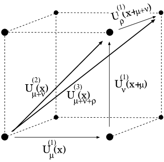
Figure 11: A 3d illustration for the construction of hyperlinks in the gauging of a hypercube fermion.

In Ref. [73] we discussed a suitable preconditioning method for the HF. The goal is to divide the lattice into sublattices such that a block structure in the lattice Dirac operator $D_{x,y}(U)$ is generated. This block structure allows for the transition to an equivalent Dirac operator with a better condition number. This means that the ratio between the maximal and minimal eigenvalue of $D^{\dagger}D$ decreases, and this ratio is essential for the computational effort in a simulation. Moreover, the transformed operator is block diagonal, which also simplifies its inversion.

For the Wilson fermion, this method is usually applied with two sublattices, which do not contain nearest neighbour sites, as distinguished by the sign term (3.30). It is known as even-odd (or red-black) preconditioning. For the HF a set of $2^{d}$ sublattices is suitable, which we denoted as “rainbow preconditioning”. In fact, it yields gain factors between 3 and 4 in typical QCD simulations [73]. (We add that also for Wilson fermions it can be profitable to deal with a larger set of sublattices, as the locally-lexicographic symmetric successive overrelaxed preconditioner (ll-SSOR) shows [74].)

6.2 Approximate rotation symmetry

A first simulation of this HF with the simple gauging described above was presented in Ref. [50]. We set the bare fermion mass to zero and evaluated the dispersion relation for the pseudoscalar meson with the Wilson plaquette gauge action (see e.g. Refs. [28]), at $\beta=5$ in a quenched simulation on a lattice of size $6^{3}\times 18$. The corresponding “speed of light”

$$c_{\rm meson}=\frac{\sqrt{E^{2}-M^{2}}}{|\vec{p}\,|}$$ (6.1)

is shown in Figure 12 and compared to the result for the Wilson fermion. In this formula, $E$, $M$ and $\vec{p}$ are the energy, mass and 3-momentum of the pseudoscalar meson. The continuum behaviour, $c_{\rm meson}=1$, is marked by a dotted line. We see that it is approximated very well for the HF — which leads to $c_{\rm meson}=1.04(5)$ — in striking contrast to the Wilson fermion. This property corresponds to an excellent approximation to Lorentz symmetry (resp. to Euclidean rotation invariance).

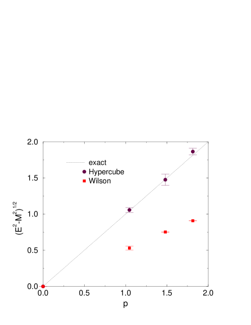
Figure 12: The “speed of light” in eq. (6.1) determined from the dispersion relation of a pseudoscalar meson on the lattice. We see that the continuum relation $c_{\rm meson}=1$ is approximated very well for the HF, but not for the Wilson fermion [50]. The simulation was performed quenched with the Wilson gauge action at $\beta=5$.

However, the meson mass is strongly renormalised in this case. In lattice units it amounts to $M\simeq 3$, hence it can hardly describe a pion. Of course, we were dealing with a very coarse lattice. Still, this property calls for a closer look at chiral symmetry, which we will undertake in Section 7.

The HF has been applied successfully in simulations of the Schwinger model [72] with two flavours, on a $16\times 16$ lattice at $\beta=6$, $4$ and $2$ [75]. In these simulations, the gauge configurations where generated quenched, but the measurements did include the fermion determinant. We used the Wilson plaquette gauge action, which is perfect for pure 2d $U(1)$ gauge theory (see Subsection 5.3).

First we present another test of the quality of rotation symmetry. Figure 13 shows the decay of the correlation function

$$C_{3}(x)=\langle\bar{\Psi}_{0}\,\sigma_{3}\Psi_{0}\cdot\bar{\Psi}_{x}\,\sigma_{3}\Psi_{x}\rangle\$$ (6.2)

against the distance $|x|$, where $x$ are lattice sites in all directions. We measured this correlator for the Wilson fermion and for several types of 2d HFs, which are described in Ref. [75]. For the TP-HF, the fermionic couplings correspond exactly to the description in Subsection 4.1, whereas the SO-HF is further optimised with respect to the scaling behaviour. Both variants also include a clover term. This plot shows in addition the results obtained with the classically perfect action constructed in Ref. [13].

The observation that the HFs and the (far more complicated) classically perfect action display a much smoother decay of $C_{3}$ down to short distances $|x|$ approves their good approximation to rotation symmetry.

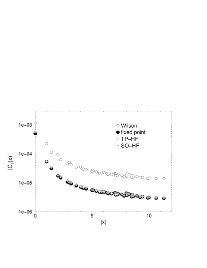
Figure 13: The isotropic correlation function (6.2) for the Wilson fermion, a fixed point fermion and two HF versions in the Schwinger model. We see in all cases but the Wilson fermion a smooth decay, which confirms the good quality of approximate rotation symmetry down to short distances.

6.3 Spectral properties in the two-flavour Schwinger model

6.3.1 Applications of the hypercube fermion

In Ref. [75] we also measured the dispersion relations for the states, which are analogous to the pion and the $\eta$-meson (a general discussion of these properties of the Schwinger model can be found in Ref. [76]). Again, for increasing momenta (in lattice units) scaling errors due to lattice artifacts are enhanced, cf. Subsections 2.2 and 4.1. In Figure 14 we show these dispersions, which are again strongly improved for the classically perfect action and for the HFs, in particular for the SO-HF. It is remarkable that the latter — which is still very simple — scales at least as well as the highly involved classically perfect action of Ref. [13].

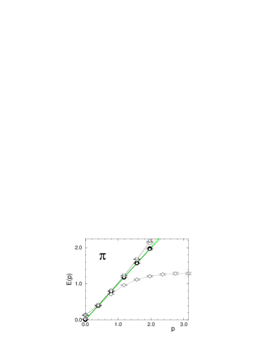
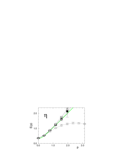
Figure 14: The dispersion relations for the “pion” and the “$\eta$-meson” in the Schwinger model with various lattice fermion formulations: Wilson fermions (diamonds), the classically perfect action (filled circles) and three types of HFs, in particular the scaling optimised SO-HF (little empty boxes) [75]. The solid lines mark the behaviour in the continuum.

6.3.2 Applications of a truncated perfect staggered fermion

In Ref. [77] we constructed with a similar procedure a truncated perfect staggered fermion, starting from the formulation described in Subsection 4.2. We applied it in Schwinger model simulations as well, and these simulations were truly dynamical. We designed a variant of the Hybrid Monte Carlo algorithm [78], which is particularly suitable for this formulation. It uses a simplified action (the standard staggered fermion action with fat links) for the Molecular Dynamics, and the full quasi-perfect action in the Metropolis accept/reject step. This provided a numerically cheap evaluation of the force, along with a still useful acceptance rate (as expected, the latter decreases at strong gauge coupling, which corresponds to a large physical volume). Again we used a $16\times 16$ lattice and the plaquette gauge action. At $\beta=3$ we found the neat $\pi$ and $\eta$ dispersion relations shown in Figure 15.

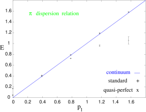
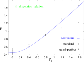
Figure 15: The dispersion relations for the “pion” and the “$\eta$-meson” in the 2-flavour Schwinger model with dynamical staggered fermions. We show results for standard staggered fermions and for truncated perfect staggered fermions [77], similar to the HF discussed before. The solid lines mark the behaviour in the continuum, which is also here very close to the data for the truncated perfect action.

In the framework of that project, we further investigated the “meson” masses under variation of the gauge coupling $\beta$ (the parameters are given in detail in Ref. [77]). The results, shown in Figure 16, reveal again that the truncated perfect formulation is far more suitable to approximate the continuum behaviour, and in particular to realise light pions — even on coarse lattices.

Figure 16: The “meson” masses in the Schwinger model from dynamical simulations with different types of staggered fermions, at various values of $\beta$, resp. lattice spacings $a\propto 1/\sqrt{\beta}$. We confirm that the results for the truncated perfect staggered fermion are far closer to the continuum results, and they provide much lighter “pions”.

This work has pioneered on one side the construction and application of improved staggered fermions — which became indeed fashion in the beginning of this century — as well as the use of a simplified force term in the Hybrid Monte Carlo simulation of a complicated quasi-perfect action.

6.4 The charmonium spectrum

Regarding QCD, we performed simulations to evaluate the charmonium spectrum employing the HF [79]. In this case we used a truncated version of the perfect quark gluon vertex function discussed in Subsection 5.4. The result is shown in Figure 17. This was a quenched simulation with the Wilson gauge action at $\beta=5.6$ on a $8^{3}\times 16$ lattice. The bare quark mass was set to $m=0.9$ — that value was adapted to match the ground state $\eta_{c}(2.98{\rm GeV})$. Considering the fact that only this ground state was used as an input, the agreement with the experimental spectrum is clearly satisfactory. The inclusion of a term $\propto\gamma_{\mu}\gamma_{\nu}\gamma_{\rho}$ in the vertex function (see also Ref. [50]) was especially helpful for the quality of the charmonium spectrum.

Figure 17: The charmonium spectrum, measured in simulations with the HF and a truncated perfect quark gluon vertex function [79]. The experimental values are dashed, and the ground state of $\eta_{c}$ sets the scale.

6.5 Spectral functions at finite temperature

At last, we add that the HF is currently being applied in studies of the spectral functions of QCD at finite temperature [80, 81]. These spectral functions, depending on the frequencies, are obtained from lattice data using the Maximum Entropy Method, which was suggested for this purpose in Ref. [82]. For the HF they reveal a continuum-like behaviour up to much larger energies than it is the case for the Wilson fermion, see Figure 18. The basis for this virtue is that the HF moves all the doublers to a unique cutoff scale, whereas the Wilson fermion splits them into four (in general $d$) subsets, see Subsection 7.5. We recall that the naive doubler species have between $1$ and $d$ momentum components $\pi/a$ in the free case. This causes the splitting in their cutoff energy for $D_{\rm W}$ — an effect that $D_{\rm HF}$ overcomes.

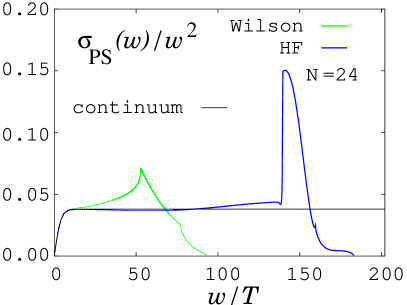
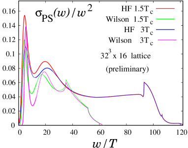
Figure 18: The spectral function $\sigma_{\rm PS}$, as a function of the frequencies $\omega$, at critical temperature $T_{c}=\infty$ (on the left, free case) and at finite $T_{c}$ (on the right, interacting case). These results are obtained from lattice data using the Maximum Entropy Method for the HF and for the Wilson fermion.

7 Chiral Correction by means of the Overlap Formula

7.1 The Ginsparg-Wilson relation

In Subsection 4.1 we discussed the block variable RGT for the free fermion field. Eq. (4.2) introduced the transformation term, which we assume (for simplicity) to be diagonal in the spinor indices,

$$\sum_{x,y}\Big{[}\bar{\Psi}_{x}-\int_{C_{x}}d^{d}u\,\bar{\psi}(u)\Big{]}(R^{-1})_{xy}\Big{[}\Psi_{y}-\int_{C_{y}}d^{d}v\,\bar{\psi}(v)\Big{]}\ .$$ (7.1)

For the bare fermion mass $\,m=0\,$ the inverse perfect lattice Dirac operator has the structure

$$(D^{-1})=\frac{-\gamma_{\mu}\rho_{\mu}}{\rho^{2}+\lambda^{2}}+R\ ,\quad R=\frac{\lambda}{\rho^{2}+\lambda^{2}}\ ,$$ (7.2)

where we are using the notation of eq. (4.7) and $\rho^{2}=\rho_{\nu}\rho_{\nu}$ (in coordinate space, the products are lattice convolutions). We repeat that in the limit of a $\delta$-function RGT, $R\to 0$, the lattice action is invariant under the standard chiral transformation (3.14), as we see from the anti-commutator $\{D,\gamma_{5}\}=0$.

However, we also saw that locality requires $R\neq 0$, in agreement with the Nielsen Ninomiya No-Go Theorem [22], and we found for $m=0$ the term

$$R_{xy}=\frac{1}{2}\delta_{xy}$$ (7.3)

to be optimal for locality [15]. In this case, we have to face $\{D,\gamma_{5}\}\neq 0$, but due to our requirements for $R$ in Subsection 4.1 (eq. (4.5)) the anti-commutator

$$\{D^{-1},\gamma_{5}\}=2\gamma_{5}R$$ (7.4)

is local. The exact form of the factor $\Pi$ (which depends on the blocking scheme, for our case it is given in eqs. (4.3) and (2.11)) does not affect this relation. This already indicates that for a given term $R$ there is a variety of solutions to eq. (7.4).

We stressed in Section 4 — and a long time ago, for instance in Ref. [46] — that the specific chiral symmetry breaking by the term $R$ cannot distort any physical properties, in particular not those related to chirality. Relation (7.4) illustrates this again, since a local term $R$ cannot shift the poles in the propagator $D^{-1}$. If we multiply the operator $D$ from both sides, we arrive at the equivalent equation

$$\{D,\gamma_{5}\}=2D\gamma_{5}RD\ ,$$ (7.5)

which is now known as the Ginsparg-Wilson relation (GWR). The dimensions reveal that the right-hand side is $O(a)$ suppressed. As we mentioned earlier, the GWR was written down in Ref. [44], which was forgotten over a long period until its re-discovery in 1997 [45].

We may compare this property to the Wilson operator, which breaks chiral symmetry such that $\{D_{{\rm W},m=0},\gamma_{5}\}$ amounts to a local term, unlike relation (7.4). If we try to insert the free operator $D_{{\rm W},m=0}$ into the GWR, we arrive at a non-local term $R_{xy}$, which decays only as $|x-y|^{-6}$ in $d=4$, and as $|x-y|^{-4}$ in $d=2$ [83]. Hence the Wilson operator does not solve the GWR.

We continue to use the GWR as a requirement also in the interacting case. For gauge interactions, $D(U)$ involves the link variables, and so does $R$, if it couples different lattice sites. However, we stay now with the choice (7.3), for which the GWR takes the simple form

$$R_{xy}=\frac{1}{2}\,\rho\,\delta_{xy}\ ,\ \rho=1\quad\Rightarrow\quad\{D,\gamma_{5}\}=D\gamma_{5}D\ .$$ (7.6)

M. Lüscher observed that this relation assures the exact invariance under a lattice modified chiral symmetry transformation [49]. In the notation of eq. (3.14), it is sufficient to consider this modified transformation to $O(\alpha)$ (due to the Lie group structure of the chiral rotation),

$$\bar{\Psi}D\Psi \to \bar{\Psi}\Big{(}1+\alpha(1-\frac{1}{2}D)\gamma_{5}\Big{)}\,D\,\Big{(}1+\alpha\gamma_{5}(1-\frac{1}{2}D)\Big{)}\Psi+O(\alpha^{2})$$ (7.7)

$$= \bar{\Psi}D\Psi+\alpha\bar{\Psi}\Big{[}\{D,\gamma_{5}\}-D\gamma_{5}D\Big{]}\Psi+O(\alpha^{2})\ .$$

The GWR corresponds exactly to a vanishing term in the square bracket. In fact, it could have been also discovered by requiring invariance under such a lattice modified chiral symmetry. Unlike the remnant chiral symmetry of staggered fermions, this chiral rotation involves the full number of generators that appear in the continuum theory. The continuum limit $a\to 0$ yields a smooth transition to the standard form of chiral invariance. Based on these observations, even a non-perturbative formulation of chiral $U(1)$ gauge theory (cf. Subsections 3.3 and 3.4) has been worked out on the conceptual level [84]. Earlier works in this direction, based on the overlap formalism, are collected in Ref. [85].

Perfect Dirac operators solve the GWR, but — as we saw — they can in general not be constructed explicitly. A step towards an applicable solution was the observation that also classically perfect Dirac operators (cf. Subsection 2.3) are Ginsparg-Wilson operators [86]. Still, a truncation of the couplings and therefore a deviation from exact chiral symmetry is needed in its construction, but in view of the possibilities to build approximate solutions this is a more accessible starting point than the (quantum) perfect action.

A fully explicit solution was presented by H. Neuberger [87]. Let us recall the properties (3.16) and start from some massless lattice Dirac operator $D_{0}$, which we assume to be $\gamma_{5}$-Hermitian, i.e.

$$D^{\dagger}_{0}=\gamma_{5}D_{0}\gamma_{5}\ .$$ (7.8)

This property holds for practically all Dirac operators that have been considered, in particular for the Wilson operator $D_{\rm W}$. Now we define the shifted operator

$$A:=D_{0}-1\ ,$$ (7.9)

which is unitary if  $D_{0}$ is a GW operator,

$$A^{\dagger}A=\gamma_{5}\Big{[}D_{0}\gamma_{5}D_{0}-\{D_{0},\gamma_{5}\}+\gamma_{5}\Big{]}\ .$$ (7.10)

Of course, we cannot assume this for a quite general $D_{0}$, and we pointed out before that it does not hold in particular for $D_{\rm W}$. But we can transform $A$ such that unitarity is enforced,

$$A\to A_{\rm ov}:=A/\sqrt{A^{\dagger}A}\ \quad\Rightarrow\quad A_{\rm ov}^{\dagger}A_{\rm ov}=1\!\!1\ .$$ (7.11)

In this way, we obtain the overlap Dirac operator

$$D_{\rm ov} = 1+A_{\rm ov}=1+(D_{0}-1)/\sqrt{(D_{0}^{\dagger}-1)(D_{0}-1)}$$ (7.12)

$$= 1+\gamma_{5}\frac{H}{\sqrt{H^{2}}}\ ,\quad H:=\gamma_{5}A\ ,$$

where $H$ is Hermitian, $H=H^{\dagger}$. H. Neuberger introduced this operator [87] with $D_{0}=D_{\rm W}$, and we denote the corresponding overlap operator as the Neuberger operator $D_{\rm N}$.

Since the resulting lattice action $S[\bar{\Psi},\Psi,U]$ has now a modified but exact chiral symmetry, one may be worried about the fate of the axial anomaly. However, the anomaly is in fact captured correctly, due to the variance of the functional measure under modified chiral rotations [49], which is analogous to the continuum. This property means an explicit realisation of the program formulated in Ref. [89]. The axial anomaly has been computed perturbatively by many authors, for instance in Refs. [44, 49, 86, 90] for general Ginsparg-Wilson operators, and specifically for $D_{\rm N}$ also in Refs. [91]. A proof which extends to all topological sectors was given for $D_{\rm N}$ in Ref. [92]. In fact, this extension is non-trivial, as the considerations in Refs. [93] underline.

7.2 Massless lattice fermions in $d=3$

In three dimensions, there is no chiral symmetry (since there is no matrix $\gamma_{5}$ at hand), but parity takes a rôle similar to a discrete chiral symmetry. The parity operator ${\cal R}$ is then the analogue to $\gamma_{5}$, and we can write the parity transformation on the lattice for spinors and compact link variables as

$$P : \bar{\Psi}_{x}\to i\bar{\Psi}_{x}{\cal R}\ ,\quad\Psi_{x}\to i{\cal R}\Psi_{x}\ ,$$ (7.13)

$$U_{\mu,x}\to U_{\mu,x}^{P}:=U_{\mu,-x}^{\dagger}\ .$$

Similar to the $\gamma_{5}$-Hermiticity (7.8), practically all lattice Dirac operators which are considered obey

$$D(U)^{\dagger}={\cal R}D(U^{P}){\cal R}\ .$$ (7.14)

The relation

$$D(U)+D(U)^{\dagger}=0\$$ (7.15)

then implies parity invariance of the action $S=\sum_{xy}\bar{\Psi}_{x}D(U)_{xy}\Psi_{y}$, and fermion mass zero. However, this condition (7.15) is again not easy to fulfil — it leads to a doubling problem as the chiral symmetry does in even dimensions. The doublers in the naive action can be avoided by a Wilson term, but this term breaks the condition (7.15) and therefore parity symmetry, so that additive mass renormalisation sets in.

A (massless) overlap fermion in $d=3$ was introduced in Ref. [94], which was actually the first place where the overlap formula (7.12) appeared. In Ref. [95] we considered generally a 3d Ginsparg-Wilson operator given by the condition

$$D+D^{\dagger}=D^{\dagger}D\ ,$$ (7.16)

and we studied a lattice modified parity symmetry. This modification alters the transformations (7.13) such that

$$\Psi_{x}\to i{\cal R}(1-D)\Psi_{x}\ .$$ (7.17)

For a solution $D$ to eq. (7.16) the lattice action is exactly invariant under this modified parity symmetry, but the functional measure transforms as

$${\cal D}\bar{\Psi}\,{\cal D}\Psi\ \to\ [{\rm det}(1-D)]^{-1}{\cal D}\bar{\Psi}\,{\cal D}\Psi\ .$$ (7.18)

Once more in analogy to the chiral symmetry in even dimensions, this transformation of the measure gives rise to the requested parity anomaly [95]. We should clarify that this is not an anomaly in the usual sense, which has a unique value, but it comes with an arbitrary integer factor (a comprehensive discussion is given in Ref. [96]). Hence a successful regularisation should capture all possibilities for this integer. In the current case, they are all captured indeed by varying either the kernel $R$ in the GWR (which then modifies the right-hand-side of eq. (7.16) to $2D^{\dagger}RD$), or by considering different kernels $D_{0}$ in the overlap formula (7.12).

At this point we add that also a pure Abelian 3d Chern-Simons gauge theory with the continuum action

$$S[{\cal A}]=\int d^{3}x\,\epsilon_{\mu\nu\rho}\,{\cal A}_{\mu}\partial_{\nu}{\cal A}_{\rho}$$ (7.19)

suffers from a doubling problem on the lattice due to the occurrence of a linear momentum [97]. A solution can be found also here either by the perfect action formalism, or by a formula of the overlap-type [98].

7.3 The overlap hypercube fermion

We proceed to a slightly more general form of the term $R$ in the GWR (7.5): we now allow for a parameter $\rho\mathop{\raise 1.29167pt\hbox{$>$\kern-7.5pt\raise-4.73611pt\hbox{$\sim$}}}1$ in eq. (7.6). The overlap formula can be adapted to general forms of $R$ [99, 14]. For the still simple form that we are considering now, it reads

$$D_{\rm ov} = \rho\left(1+A/\sqrt{A^{\dagger}A}\right)=\rho\Big{(}1+\gamma_{5}\frac{H}{\sqrt{H^{2}}}\Big{)}\ ,$$

$$A := D_{0}-\rho=\gamma_{5}H\ .$$ (7.20)

As we mentioned, the standard formulation inserts as a kernel the Wilson operator, $D_{0}=D_{\rm W}$, which is far from chiral, and which undergoes a drastic change in the overlap formula to yield the Neuberger operator $D_{\rm N}$. Ref. [99] suggested to consider more general possibilities for $D_{0}$, and motivated in particular the use of a truncated perfect operator, which is approximately chiral already. In this case, the square root in eq. (7.20) is close to the constant $\rho$, and the transition from $D_{0}$ to $D_{\rm ov}$ is therefore only a modest modification. An intuitive argument for this property is that an exact GW kernel $D_{0}$ reproduces itself identically in the overlap formula (7.20) (for a fixed parameter $\rho$).

In particular we are using $D_{\rm HF}$ as the input Dirac operator — note that it is $\gamma_{5}$-Hermitian as well. Its inexact chirality is then corrected by the overlap formula, which leads to $D_{\rm ovHF}$, the operator of the overlap-HF, while keeping both Dirac operators similar,

$$D_{\rm ovHF}\approx D_{\rm HF}\ .$$ (7.21)

The motivation for this construction is that the property (7.21) allows us to preserve other virtues of $D_{\rm HF}$ (beyond the approximate chirality) in the chirally exact formulation $D_{\rm ovHF}$. As such virtues we are going to discuss:

• a high level of locality

• approximate rotation symmetry

• a good scaling behaviour.

Below we will summarise results for these three aspects and comment on their meaning. Still before that we mention that the simulation of an overlap fermion with a hypercubic kernel requires more computational effort compared to $D_{\rm N}$. The use of the complicated kernel by itself corresponds to an overhead of about a factor $15$ in QCD (without applying the preconditioning method reviewed in Subsection 6.1). However we should consider that in 4d simulations, the inverse square root in the overlap formula (7.20) (resp. the sign function $\frac{H}{\sqrt{H^{2}}}$ ) is approximated by polynomials. Again thanks to the relation (7.21), the convergence in the polynomial evaluation is faster — for a fixed precision one gains back by this property about a factor of $3$ [102, 103, 104]. Hence an overhead of about a factor $5$ remains. We are confident that this factor will be more than compensated by the superior properties listed above, which we will discuss in Subsections 7.6 and 7.7.

7.4 The axial anomaly in the continuum limit

On the conceptual side, we were able to prove that also the overlap-HF (obtained by inserting $D_{0}=D_{\rm HF}$ in the overlap formula, as we just advocated) has the correct chiral anomaly in the continuum limit of all topological sectors [105]. This proof required a number of generalisation steps compared to the proof that had been worked out previously for the Neuberger operator $D_{\rm N}$ [92].

In Ref. [105] we gave a non-perturbative evaluation of the continuum limit of the axial anomaly and the fermion index. To this end, we formulated the Dirac operator $D_{\rm HF}$ on a $2n$-dimensional Euclidean lattice in a form, which is well-suited for analytic investigations. We used it first to study the dependence of the doubler structure of $D_{\rm HF}$ on its coupling parameters. Then we evaluated the classical continuum limits of the axial anomaly and the index of the overlap-HF operator, showing that the correct continuum expressions are recovered when the parameters are in the physical (doubler-free) range. This continuum limit relies only on general properties of $D_{\rm HF}$ and not on its explicit form (in contrast to the previous evaluations in the Wilson case [92]). The main new technical tool was a set of identities, which allowed the continuum form

$$\epsilon_{\mu_{1}\dots\mu_{2n}}\,{\rm Tr}\,F_{\mu_{1}\mu_{2}}(x)\cdots{}F_{\mu_{2n-1}\mu_{2n}}(x)$$ (7.22)

of the axial anomaly to be extracted, and its coefficient to be evaluated topologically.

These properties are basically not specific to the HF structure. We expect that this proof can be extended to completely general overlap Dirac operators obtained by inserting an ultralocal (and $\gamma_{5}$-Hermitian) lattice Dirac operator $D_{0}$ (involving the full Clifford algebra of $\gamma$ matrices, as the operators in Refs. [14, 101, 106]) into the overlap formula.

7.5 Approximate chirality of the hypercube fermion

An exact solution to the GWR with a term $R$ of the form (7.5) and $\rho\mathop{\raise 1.29167pt\hbox{$>$\kern-7.5pt\raise-4.73611pt\hbox{$\sim$}}}1$ has its spectrum $\sigma(D)$ on a circle in the complex plane with centre and radius $\rho$, as we see from the relation $A^{\dagger}A\equiv\rho^{2}$. We call it the GW circle,

$$\sigma(D)\subset\Big{\{}z\ \Big{|}\ |z-\rho|=\rho\Big{\}}\ .$$ (7.23)

This property reveals immediately the absence of additive mass renormalisation and of “exceptional configurations” (with accidental near-zero modes in quenched simulations). In order to check how well some input operator $D_{0}$ approximates chirality already, it is therefore a sensible criterion to evaluate the spectrum $\sigma(D_{0})$ and to test if it is close to this GW circle [99]. Let us start with the free HF in $d=4$: the spectrum of $D_{\rm HF}$ in infinite volume is shown in Figure 19, and we see that it approximates the GW circle (with $\rho=1$) extremely well. On the other hand, the spectrum of the free Wilson operator covers four circles of this kind, so that its real part extends up to $\approx 8$.  (We anticipated this property in Section 6 when we commented on Figure 18.)

Figure 19: The spectrum of the truncated perfect, free HF in $d=4$, on a lattice of unit spacing and infinite size. It is very close the GW circle with centre and radius $\rho=1$, which shows that it approximates chirality very well.

To study this property in the presence of gauge interactions, we first return to the 2-flavour Schwinger model. We considered this model as described in the first part of Subsection 6.3, and we show the spectrum of a typical configuration at $\beta\equiv 1/g^{2}=6$ for $D_{\rm W}$ and for $D_{\rm HF}$ in Figure 20 [75]. In two dimensions, the spectrum of $D_{\rm W}$ covers the vicinity of two circles, whereas the HF is again very close to the GW circle with $\rho=1$. As an experiment, we also show in the latter case the spectrum after a minimal approximation to the overlap formula: we only use its first term in the Taylor expansion, which leads to a spectrum that can hardly be distinguished from the exact GW circle.

Figure 20: The spectra of the Wilson operator (with and without a clover term with coefficient $1$) and of the HF operator for a typical configuration in the Schwinger model at $\beta=6$. The Wilson spectrum deviates strongly from the GW circle, whereas the HF spectrum approximates it well. In the latter case we also show the result if the overlap formula is approximated by a polynomial of first order only, which is sufficient to put the eigenvalues quite exactly onto the GW circle [75].

As we increase the strength of the gauge coupling $1/\sqrt{\beta}$, the eigenvalues spread out a bit more, but they still follow closely the GW circle for $\beta=4$ and even $\beta=2$, as we illustrate in Figure 21.

Figure 21: The spectra of the HF operator for typical configurations in the Schwinger model at $\beta=4$ and at $\beta=2$. The GW circle is still approximated well. We also show a polynomial correction with the Taylor expanded overlap formula to the first resp. second order.

In QCD this property is more tedious to achieve. Refs. [107, 102] describe the construction of a suitable HF formulation for quenched QCD at $\beta\equiv 6/g^{2}=6$. It starts again from the free, truncated perfect HF and restores approximate criticality under gauge interaction by a link amplification $U_{x,\mu}\to uU_{x,\mu}$, $u\mathop{\raise 1.29167pt\hbox{$>$\kern-7.5pt\raise-4.73611pt\hbox{$\sim$}}}1$. Further ingredients are a separate link amplification factor $v$ for the vector term (which controls the imaginary part of the spectrum, with hardly any effect on the mass renormalisation), and the simplest version of a “fat link”. The latter amounts to the substitutions

$$U_{x,\mu}\to(1-\alpha)U_{x,\mu}+\frac{\alpha}{6}\ \sum\ [\ {\rm staples~{}terms}\ ]$$ (7.24)

for all compact link variables, where we chose $\alpha$ in the range $0.3\dots 0.5$. The fat link helps to pull the eigenvalues around real part $1$ somewhat closer to the GW circle [107, 102]. At some point, also a clover term was considered, but since its optimisation led to a coefficient close to $0$ we dropped it again. We arrived at a very satisfactory approximation for typical configurations at $\beta=6$, as Figure 22 shows. This plot includes the full spectrum on a $4^{4}$ lattice, as well as the low eigenvalues on a $8^{4}$ lattice, which fill the gap near zero (this gap is generic on small lattices).

Figure 22: The spectrum of the optimised HF operator for a typical configuration in quenched QCD at $\beta=6$ on lattices of the sizes $4^{4}$ (crosses, full spectrum) and $8^{4}$ (squares, physical part of the spectrum).

Later on, such a construction was also accomplished at $\beta=5.85$, i.e. on a coarser lattice, where it is more difficult. Still this program could be carried out successfully [103, 104]. In this case, we made a compromise between the criteria of a minimal condition number of $A^{\dagger}A$ and optimal locality of $D_{\rm ovHF}$ (to be discussed in this and the following Subsection).

An immediate consequence of the approximate chirality of $D_{\rm HF}$ is that the polynomial evaluation of $D_{\rm ovHF}$ (to a fixed precision) is faster, i.e. the required degree is lower, as we mentioned before. In QCD we used Chebyshev polynomials for this purpose, which converge exponentially as the degree rises (see e.g. Ref. [109]). The required degree is then proportional to the square root of the condition number of the operator $A^{\dagger}A$. In practice one usually projects out the lowest few modes and treats the eigenspace spanned by them separately — this reduces the condition number of the remaining operator very significantly. Figure 23 compares these condition numbers for the Neuberger operator and the overlap-HF, for QCD on a $12^{4}$ lattice at $\beta=6$, with $k-1=1\dots 19$ modes projected out. We recognise for the overlap-HF a gain factor $\approx 25$, which we anticipated at the end of Subsection 7.3. This gain factor is essentially due to the reduction of the maximal $A^{\dagger}A$ eigenvalue, and it persists practically unchanged at $\beta=5.85$; details can be found in Ref. [104] (Table 1).

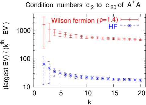
Figure 23: The condition numbers of the overlap ingredient $A^{\dagger}A=H^{2}$, where $H$ is the Hermitian operator $H=\gamma_{5}A$ (and $A=D_{0}-\rho$, see eq. (7.20)), for the Neuberger operator and for the overlap-HF, in QCD on a $12^{4}$ lattice at $\beta=6$. $k-1$ is the number of lowest modes which are projected out. The condition number of the remaining operator, i.e. the ratio $c_{k}={\rm(largest~{}eigenvalue~{}of~{}}A^{\dagger}A)/(k^{\rm th}{\rm~{}eigenvalue~{}of~{}}A^{\dagger}A)$, is about $25$ times lower for the overlap-HF [102], from which we infer a gain factor of about $5$ in the polynomial degree. The computational effort is roughly proportional to this degree.
This gain factor is practically the same at $\beta=5.85$ on a $12^{3}\times 24$ lattice [104].

7.6 Locality and rotation symmetry

Now we move on to the point where the overlap operator is already evaluated to a high accuracy of at least $10^{-12}$ (in many case, the precision was also set to $10^{-15}$ or $10^{-16}$). First we compare the level of locality of the overlap-HF to the standard formulation $D_{\rm N}$. A strong gain in this level was first observed for the free fermion in Ref. [99], which was one of the motivations to generalise the overlap operator, as described in Subsection 7.3. In Figure 24 we show this property in $d=2$: on top we see that the couplings in $D_{\rm ovHF}$ decay much faster than in $D_{\rm N}$. Since the $D_{\rm ovHF}$ couplings follow closely a single exponential curve, this plot also illustrates an improved rotation symmetry. Both properties can be understood based on the ultralocality and the good rotation symmetry of $D_{\rm HF}$, together with relation (7.21). (Of course, ultralocality also holds for $D_{\rm W}$, but the relation (7.21) does not, hence this property is not approximately inherited in $D_{\rm N}$.) In fact, the level of locality is related to the minimal separation of a $D_{0}$ eigenvalue from $\rho$ (the centre of the GW circle) [112]; this implies a link between the quests for locality of an overlap operator and approximate chirality of its kernel $D_{0}$. The optimal parameters have roughly the same trend for these criteria, but they are not identical (we mentioned in the previous Subsection that we made a compromise between maximal locality of $D_{\rm ovHF}$ and minimal condition number of $A^{\dagger}A$).

In the lower plot in Figure 24 we see that the superior locality of $D_{\rm ovHF}$ persists in the Schwinger model at $\beta=6$ [75]. In this case we measure the locality in the way suggested in Ref. [112]: we put a unit source $\eta_{y}$ at one site $y$, and we consider all sites $x$ separated from $y$ by a taxi driver distance $r=\sum_{\mu}|x_{\mu}-y_{\mu}|:=\|x-y\|_{1}$. Then we identify the maximum of the norm $\|D_{xy}\eta_{y}\|$, which we denote as $f(r)$,

$$f(r)=\ ^{\rm max}_{~{}\,x}\Big{\{}\|D_{xy}(U)\eta_{y}\ \Big{|}\ \|x-y\|_{1}=r\Big{\}}\ .$$ (7.25)

The exponential decay of $\langle f(r)\rangle$ in $r$ is a compelling criterion to demonstrate locality. For $\beta=6$ we see in Figure 24 (below) that this decay is much faster for $D_{\rm ovHF}$ than for $D_{\rm N}$.

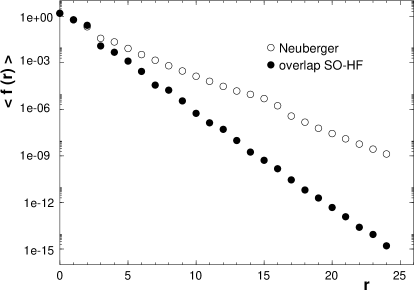
Figure 24: The locality of the overlap-HF vs. the standard Neuberger operator in $d=2$. On top we show the decay of the free couplings in the vector term $\rho_{\mu}$ and in the scalar term $\lambda$ (in the notation $D_{\rm ov}=\rho_{\mu}\gamma_{\mu}+\lambda$), against the Euclidean distance $|x|$. We see that the overlap-HF couplings follow a much faster exponential decay, indicating a higher level of locality. Moreover, the couplings in the Neuberger operator are much more spread out, which reveals a better approximate rotation symmetry for the overlap-HF.
Below we compare the locality in the Schwinger model at $\beta=6$, measured according to eq. (7.25) (in the taxi driver metrics). We see that the overlap-HF is still by far more local.

We proceed to QCD and first illustrate that we obtain again a higher degree of locality for the overlap-HF at $\beta=6$ [102] and at $\beta=5.85$ [103, 104], see Figure 25. On top, at $\beta=6$ (which corresponds to a physical lattice spacing of about $a\simeq 0.093~{}{\rm fm}$) we still use the taxi driver metrics, but below ($\beta=5.85$, corresponding to $a\simeq 0.123~{}{\rm fm}$) we switch to the Euclidean metrics. The observation that the decay for the overlap-HF is not only faster, but in the Euclidean metrics also smoother, confirms again that our overlap-HF formulation is both, more local and to a better approximation rotation invariant than the standard formulation. We add that the quality of rotation symmetry was also tested directly in the Schwinger model with the procedure shown before for the HF in Figure 13. For the overlap-HF a smooth decay of the isotropic correlator $C_{3}$ was found, similar to the HF, affirming an improved rotation symmetry [75].

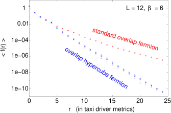
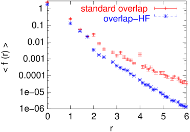
Figure 25: The locality of the overlap-HF vs. the standard operator $D_{\rm N}$ in QCD. On top the decay is compared in the taxi driver metrics at $\beta=6$, where we find a gain factor of almost $2$ in the exponent of the decay [102].
The plot below refers to $\beta=5.85$ in the Euclidean metrics, which also provides a comparison of the quality of rotation symmetry [104].

At last we turn to strong gauge couplings, which correspond to rough configurations and therefore to coarse lattices. Generally, the overlap formula is only applicable to generate a valid lattice Dirac operator up to a certain coupling strength, where locality collapses. We see in Figure 26 that the Neuberger operator is still local at $\beta=5.7$ (corresponding to $a\simeq 0.17~{}{\rm fm}$), but at $\beta=5.6$ no exponential decay can be observed anymore (for any parameter $\rho$). In contrast, the overlap-HF (where only the link amplification factor is adapted compared to the formulation at $\beta=5.85$) is local in both cases, and at $\beta=5.7$ the function $\langle f(r)\rangle$ still exhibits a remarkably fast decay.

This superior locality is essentially due to the HF structure of the overlap kernel. By means of fat links alone the locality of the overlap operator can also be improved, but only marginally [115] (assuming the optimal value of $\rho$ in each case).

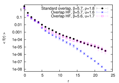
Figure 26: The locality of the overlap-HF (with a link amplification factor $u$ and $\rho=1$) vs. the Neuberger operator $D_{\rm N}$, in QCD at strong coupling (in taxi driver metrics). At $\beta=5.7$ $D_{\rm N}$ (with an optimised parameter $\rho=1.8$) is still local, but at $\beta=5.6$ its locality — and therefore its validity as a lattice Dirac operator — collapses. The overlap-HF is local in both cases. At $\beta=5.7$ its locality is still stronger than the one of $D_{\rm N}$ at $\beta=6$ and $\rho=1.4$ (which is optimal for locality in that case [112]).
These measurements were done on a $12^{3}\times 24$ lattice, and the anisotropy causes the bending down at large $r$.

7.7 The scaling behaviour

Again referring to the perfect action background of the HF and to relation (7.21), we also expect a good scaling behaviour for the overlap-HF. For the free overlap-HF, this is clearly confirmed by the dispersion relation, which we show for momenta $\vec{p}=(p_{1},0,0)$ in Figure 27. In contrast, $D_{\rm N}$ scales worse than the Wilson operator $D_{\rm W}$ in this case. Qualitatively the same behaviour is observed for massive overlap fermions [75]. We also repeated the thermodynamic scaling tests described earlier (in Subsection 4.1, before applying the overlap formula). The results in $d=2$, for three version of the overlap-HF, are by far improved compared to the standard overlap operator, see Figure 28 [75]. Here we incorporated the chemical potential also for the overlap fermions according to the prescription (4.11); for an alternative method and first simulations, see Ref. [116].

Figure 27: The dispersion relation of the free, massless overlap-HF (scaling optimised version), compared to the continuum and to the standard overlap formulation $D_{\rm N}$. These dispersions end when the argument of the square root becomes negative. To provide an overview we also include the dispersion for the kernel operators $D_{\rm HF}$ and $D_{\rm W}$.

Figure 28: The thermodynamic scaling ratios ${\rm pressure}/{\rm(temperture)}^{2}$ and ${\rm pressure}/{\rm(chemical~{}potential)}^{2}$ for free overlap fermions in $d=2$. The hierarchy of the scaling behaviour is confirmed in all respects.

In the interacting case, we reconsidered the “meson” dispersion relations in the Schwinger model (cf. Subsection 6.3), this time for exact Ginsparg-Wilson operators. Also here we observe a scaling behaviour which is by far better for the overlap-HF than for the Neuberger operator, as Figure 29 shows. Further scaling tests in the Schwinger model with the dynamical HF and the quenched re-weighted overlap-HF can be found in Ref. [117] (they were compared to the scaling with dynamical Wilson fermions, which has also been investigated in Ref. [118]). In QCD, a systematic scaling test is tedious and still outstanding, but the toy model results summarised here raise optimism also in that respect.

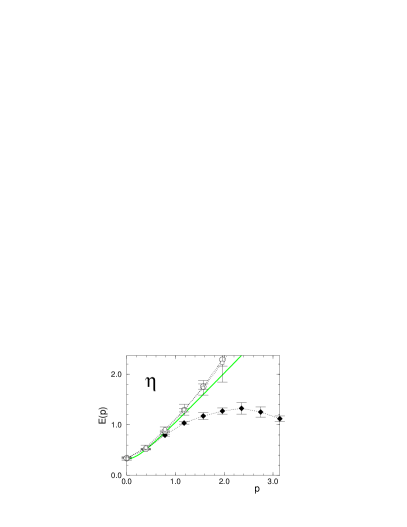
Figure 29: The mesonic dispersion relation in the Schwinger model with two types of overlap-HFs (open circles and squares). Both, the “pion” (on the left) and the “$\eta$-particle” (on the right) display a scaling which is by far improved for the overlap-HFs compared to the standard overlap fermion (diamonds). Once more we obtain the best scaling by inserting the (scaling optimised) SO-HF into the overlap formula (squares) [75].

7.8 The link to domain wall fermions

Finally we remark that the overlap fermion is equivalent to the domain wall fermion [119] in the limit of an infinite number $L_{s}$ of layers in a fifth direction. It is then a practical issue if one tries to approximate this limit by a satisfactory number $L_{s}$, or by a sufficiently precise polynomial approximation to the overlap formula. Also in the case of the domain wall fermions, the standard formulation inserts a Wilson kernel. Replacing it by a HF kernel, as suggested in Ref. [99], could lead to similar improvements as we demonstrated in this Section for the overlap fermion. The improved condition number of the kernel operator manifests itself here in a lower demand for $L_{s}$ (for some required precision of chirality). Furthermore the gains in locality, approximate rotation symmetry and scaling are expected here in practically the same form as in the overlap case.

8 Relating QCD Simulations to Chiral Perturbation Theory

8.1 Chiral Perturbation Theory

We start this Section with a few general remarks on Chiral Perturbation Theory ($\chi$PT), an effective low energy theory, which we are going to relate to our QCD simulation results.

When a continuous, global symmetry breaks spontaneously, we obtain a continuous set of degenerate vacuum states. Expanding around one selected vacuum, one distinguishes between excitations to higher energy (which are identified with massive particles) and fluctuations, which preserve the ground state energy. The subgroups of the energy conserving symmetry group can either transfer the selected vacuum to a different vacuum state, or leave it simply invariant. The number of generators relating different vacuum states corresponds — according to the Goldstone Theorem [120] — to the number of massless Nambu-Goldstone bosons (NGBs) involved. At low energy, the NGBs can be described by an effective theory as fields in the coset space of the spontaneous symmetry breaking (SSB). Such effective theories still apply if we add a small explicit symmetry breaking; we then deal with light quasi-NGBs, which dominate the low energy physics. The effective Lagrangian ${\cal L}_{\rm eff}$ contains terms of the quasi-NGB fields, which obey the original symmetry, as well as the (explicit) symmetry breaking terms. All these terms are hierarchically ordered according to some low energy counting rules for the momenta and the quasi-NGB masses. A simple example for such an expansion is outlined in Subsection 8.4.1.

This concept is very general, but it was introduced in the framework of chiral symmetry breaking in QCD [121]. At zero quark masses the left- and right-handed spinors decouple (see eq. (3.12)), so ${\cal L}_{\rm QCD}$ is invariant under their independent rotation. QCD is then assumed to exhibit a chiral SSB of the pattern

$$SU(N_{f})_{L}\otimes SU(N_{f})_{R}\ \to\ SU(N_{f})_{L+R}\ ,$$ (8.1)

where $N_{f}$ is the number of quark flavours involved. $\chi$PT is the corresponding low energy effective theory [121, 122, 123]. Following the general prescription, it deals with fields in the SSB coset space, $U(x)\in SU(N_{f})$.

A small quark mass supplements a slight explicit symmetry breaking. The quasi-NGBs are then identified with the light mesons, i.e. the pions $\pi^{+},\,\pi^{0},\,\pi^{-}$ for $N_{f}=2$ — and for $N_{f}=3$ also the kaons and $\eta$-particles.

In view of our lattice study, we have to put the system into a finite volume; we choose its shape as $V=L^{3}\times T$ $\ (T\geq L)$. We will refer to the formulations of $\chi$PT in two regimes, with different counting rules for the terms in ${\cal L}_{\rm eff}[U]$. The usual case — to be addressed in Subsection 8.2 — is characterised by a large volume, $Lm_{\pi}\gg 1$, where $m_{\pi}$ is the pion mass, i.e. the lightest mass involved, which corresponds to the inverse correlation length. This is the $p$-regime, where finite size effects are suppressed, and one expands in the meson momenta and masses ($p$-expansion) [122].

The opposite situation, $Lm_{\pi}<1$, is denoted as the $\epsilon$-regime. In that setting, an expansion in the meson momenta is not straightforward, due to the dominant rôle of the zero modes. However, the functional integral over these modes can be performed by means of collective variables [123]. There is a large gap to the higher modes, which can then be expanded again, along with the meson masses ($\epsilon$-expansion) [123, 125, 126]. We will address that regime extensively in Subsection 8.4.

In both regimes, the leading order of the effective Lagrangian (in Euclidean space) reads

$${\cal L}_{\rm eff}[U] = \frac{F_{\pi}^{2}}{4}\,{\rm Tr}[\partial_{\mu}U^{\dagger}\partial_{\mu}U]-\frac{1}{2}\Sigma\,{\rm Tr}[{\cal M}(U+U^{\dagger})]+\dots\ ,$$ (8.5)

$$U\in SU(N_{f})\ ,\qquad{\cal M}=\left(\begin{array}[]{ccc}m_{u}&&\\ &m_{d}&\\ &&(m_{s})\end{array}\right)\ .$$

Throughout Section 8 we consider only the $u$- and $d$-quark, and we assume their masses to be degenerated; we denote them by $m_{q}$. The coefficients to the terms in ${\cal L}_{\rm eff}$ are the Low Energy Constants (LECs), and we recognise $F_{\pi}$ and $\Sigma$ as the leading LECs. Experimentally the pion decay constant was measured as $F_{\pi}\simeq 92.4~{}{\rm MeV}$. $\Sigma$ is not directly accessible in experiments, but its value is assumed to be in the range $(250~{}{\rm MeV})^{3}\dots(300~{}{\rm MeV})^{3}$. For instance, in the one flavour case a value around $(270~{}{\rm MeV})^{3}$ was recently obtained based on a large $N_{c}$ expansion [127].

The LECs are of physical importance, but they enter $\chi$PT as free parameters. For a theoretical prediction of their values one has to return to the fundamental theory, which is QCD in this case. Due to the notorious lack of analytic tools for QCD at low energy, the evaluation of the LECs is a challenge for lattice simulations.

The LECs in Nature correspond to their values in (practically) infinite volume, and the $p$-regime is close to this situation. However, these phenomenological values of the LECs can also be determined in the $\epsilon$-regime, in spite of the strong finite size effects. Actually one makes use exactly of the finite size effects to extract the physical LECs. Generally, we need a long Compton wave length for the pions, $1/m_{\pi}$, and in view of lattice simulations in the $p$-regime we have to use an even larger box length $L$. In this respect, it looks very attractive to work in the $\epsilon$-regime instead, where we can get away with a small volume [128].

However, such simulations face conceptual problems, which delayed their realisation until this century: first, to realise light pions the lattice fermion formulation should keep track of the chiral symmetry. Second, the $\epsilon$-regime has the peculiarity that the topology is important (in accordance with the importance of the zero modes) [129]. $\chi$PT predictions for expectation values often differ when restricted to distinct topological sectors, so it would be a drastic loss of information to sum them up. This distinction requires a sound definition of the topological charge on the lattice. In both respects, the use of Ginsparg-Wilson fermions is ideal, due to the specific properties explained in Subsections 7.1 and 8.3.

8.2 Simulations in the $p$-regime

Usually, for $\chi$PT in a finite spatial box $L^{3}$, one expects the meson momenta $p$ to be small, so that

$$p\sim\frac{2\pi}{L}\ll 4\pi F_{\pi}\ .$$ (8.6)

The term $4\pi F_{\pi}$ takes a rôle analogous to $\Lambda_{\rm QCD}$. Regarding the counting rules for the momenta and the pion mass, the condition $L\gg 1/m_{\pi}$ allows for an application of the $p$-expansion [122]. It expands in the following dimensionless ratios, which are expected to be small and counted in the same order,

$$\frac{1}{LF_{\pi}}\sim\frac{p}{\Lambda_{\rm QCD}}\sim\frac{m_{\pi}}{\Lambda_{\rm QCD}}\ .$$ (8.7)

In this Subsection we present quenched simulation results in the $p$-regime. In Ref. [104] we applied the overlap-HF (described in Section 7) at $\beta=5.85$ on a lattice of size $12^{3}\times 24$, which corresponds to a physical volume of $V\simeq(1.48~{}{\rm fm})^{3}\times 2.96~{}{\rm fm}$ (where we use again the Sommer scale [113], cf. footnote 44). We evaluated 100 propagators for each of the bare quark masses

$$am_{q}=0.01,\ 0.02,\ 0.04,\ 0.06,\ 0.08\quad{\rm and}\quad 0.1\$$

(in physical units: $16.1~{}{\rm MeV}\dots 161~{}{\rm MeV}$). At this point we re-introduce a general lattice spacing $a$. We will see that the smallest mass in this set is at the edge of the $p$-regime — even smaller quark masses will be considered in the $\epsilon$-regime (Subsection 8.4). Part of the observables presented in the current Subsection were also measured on the same lattice with the Neuberger operator $D_{\rm N}$ at $\rho=1.6$ (a preferred value at $\beta=5.85$) [130].

We include $m_{q}$ in the overlap operator (7.12) in the usual way,

$$D_{\rm ov}(m_{q})=\Big{(}1-\frac{am_{q}}{2\rho}\Big{)}D_{\rm ov}+m_{q}\ ,$$ (8.8)

which leaves the largest real overlap Dirac eigenvalue ($2\rho/a$) invariant. $m_{q}$ represents the bare mass for the quark flavours $u$ and $d$.

We first evaluate the pion mass in three different ways:

• $m_{\pi,PP}$ is obtained from the decay of the pseudoscalar correlation function $\langle P(x)P(0)\rangle$, with $P(x)=\bar{\psi}_{x}\gamma_{5}\psi_{x}$.

• $m_{\pi,AA}$ is extracted from the decay of the axial-vector correlation function $\langle A_{4}(x)A_{4}(0)\rangle$, with $A_{4}(x)=\bar{\psi}_{x}\gamma_{5}\gamma_{4}\psi_{x}$.

• $m_{\pi,PP-SS}$ is obtained from the decay of the difference

  $$\langle P(x)P(0)-S(x)S(0)\rangle\ ,\quad{\rm where}\quad S(x)=\bar{\psi}_{x}\psi_{x}$$

  is the scalar density. This subtraction is useful at small $m_{q}$, where configurations with zero modes ought to be strongly suppressed by the fermion determinant. In our quenched study, this suppression does not happen as it should, but the above subtraction in the observable eliminates the zero mode contributions, which are mostly unphysical.

The results in Figure 30 (on top) show that the pion masses follow to a good approximation the expected behaviour $m_{\pi}^{2}\propto m_{q}$. Deviations occur at the smallest masses, where we observe the hierarchy

$$m_{\pi,PP}>m_{\pi,AA}>m_{\pi,PP-SS}\ ,$$ (8.9)

in agreement with Ref. [14]. This shows that the scalar density subtraction is in fact profitable, since it suppresses the distortion of the linear behaviour down to the lightest pion mass in Figure 30,

$$m_{\pi,PP-SS}(am_{q}=0.01)\simeq(289\pm 32)~{}{\rm MeV}\ .$$ (8.10)

That mass corresponds to a ratio $L/\xi\approx 2$, which confirms that we are leaving the $p$-regime around this point. Based on the moderate quark masses in Figure 30, we find a very small intercept in the chiral extrapolation,

$$m_{\pi,PP-SS}(m_{q}\to 0)=(-2\pm 24)~{}{\rm MeV}\ .$$ (8.11)

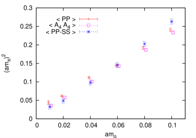
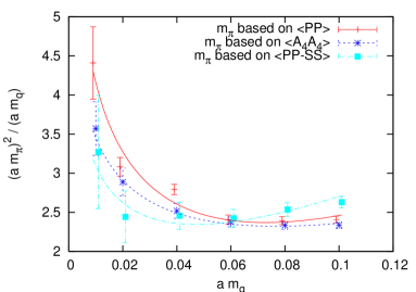
Figure 30: On top: The pion mass evaluated from overlap-HFs in the $p$-regime in three different ways, as described in Subsection 8.2.
Below: The pion masses fitted to the formula (8.12), which is expected due to the logarithmic quenching artifacts in the absence of an additive mass renormalisation.

Due to quenching, one expects at small quark masses a logarithmic behaviour of the form

$$\frac{am_{\pi}^{2}}{m_{q}}=C_{1}+C_{2}\ln am_{q}+C_{3}am_{q}\ ,\quad(C_{1},C_{2},C_{3}:~{}{\rm constants})\ .$$ (8.12)

Corresponding results are given for instance in Refs. [131, 132]. Figure 30 (below) shows the fits of our data to eq. (8.12), which works best for $m_{\pi,AA}$.

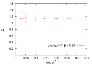
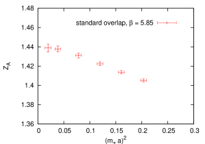
Figure 31: The axial current renormalisation constant $Z_{A}$ evaluated from $m_{\rm PCAC}$ according to eq. (8.13). For $D_{\rm ovHF}$ (on the left) we find $Z_{A}\approx 1$ [104], in contrast to the result with the standard overlap operator $D_{\rm N}$ [130] (on the right). The chiral extrapolations are given in eq. (8.14).

On the same lattice we also measured the $\rho$-meson mass in the $p$-regime using the overlap operators $D_{\rm N}$ [130] and $D_{\rm ovHF}$ [104], as well as the quark mass according to the PCAC relation,

$$m_{\rm PCAC}=\frac{\sum_{\vec{x}}\langle(\partial_{4}A_{4}^{\dagger}(x))P(0)\rangle}{\sum_{\vec{x}}\langle P^{\dagger}(x)P(0)\rangle}\ ,$$ (8.13)

where we used a symmetric nearest-neighbour difference for $\partial_{4}$. It determines the axial-current renormalisation constant $Z_{A}=m_{q}/m_{\rm PCAC}$. For the overlap-HF this constant is close to $1$ [104], see Figure 31 (on the left), which is favourable in view of the link to perturbation theory. This is in contrast to the large $Z_{A}$ value found for the standard overlap operator [130], see Figure 31 (on the right). A chiral extrapolation leads to

$$Z_{A}=1.17(2)\quad{\rm for~{}}D_{\rm ovHF}\ ,\quad Z_{A}=1.448(4)\quad{\rm for~{}}D_{\rm N}\ .$$ (8.14)

Regarding $D_{\rm N}$, consistent results were reported later in Refs. [133, 134], and (somewhat surprisingly) at $\beta=6,\ \rho=1.4$ it even rises to $Z_{A}\simeq 1.55$ [134]. When one uses the improved Lüscher-Weisz gauge action [135], the value of $Z_{A}$ for $D_{\rm N}$ is still in that range [132]. The application of fat links, however, helps to reduce $Z_{A}$ [115].

As a further observable in the $p$-regime, we measured the pion decay constant by means of the relation

$$F_{\pi}=\frac{2m_{q}}{m_{\pi}^{2}}\ \left|\langle 0|P|\pi\rangle\right|\ ,$$ (8.15)

based on $P(x)P(0)$, and based on $P(x)P(0)-S(x)S(0)$. The results for the operator $D_{\rm ovHF}$ [104] are given in Figure 32. In particular the value at $am_{q}=0.01$ (the lightest quark mass in this plot) is significantly lower for the case of the scalar subtraction. Hence this subtraction pushes the result towards the phenomenological value.

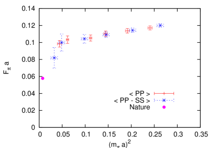
Figure 32: The pion decay constant based on a matrix element evaluation in the $p$-regime — given by eq. (8.15) — using the overlap-HF [104].

However, a chiral extrapolation based on such data for $F_{\pi}$ cannot be reliable. An extrapolated value of $F_{\pi,PP}$ would come out clearly too large, as it is also the case for $D_{\rm N}$ [130]. But in particular the instability of $F_{\pi,PP-SS}$ at our lightest pion masses in the $p$-regime (obtained at $am_{q}=\ 0.01$ and $0.02$) calls for a clarification by yet smaller quark masses. We did consider still much smaller values of $m_{q}$ in the same volume. As the results for the pion masses suggest, we are thus leaving the $p$-regime. For the tiny masses $am_{q}\leq 0.005$ we enter in fact the $\epsilon$-regime, where observables like $F_{\pi}$ have to be evaluated in completely different manners, see Subsection 8.4.

8.3 The distribution of topological charges

In the next Subsection we are going to present result in the $\epsilon$-regime of QCD. In this Subsection we focus on topological charges, which play an essential rôle the $\epsilon$-regime [129] (as we mentioned before).

As we already outlined when commenting on Figure 3, it is a priori not obvious how to introduce topological sectors on the lattice. However, if one deals with Ginsparg-Wilson fermions, a sound definition is given by adapting the Atiyah-Singer Theorem from the continuum and defining the topological charge of a lattice gauge configuration by the fermionic index $\nu$ [86],

$${\rm topological~{}charge}\,\mathop{\stackrel{{\scriptstyle!}}{{=}}}\,\nu:=n_{+}-n_{-}\ ,$$ (8.16)

where $n_{\pm}$ is the number of zero modes with positive/negative chirality. These numbers are unambiguously determined once a Ginsparg-Wilson Dirac operator is fixed (and in practice only chirality positive or chirality negative zero modes occur in one general non-trivial configuration). However, for a given gauge configuration, the index for different Ginsparg-Wilson operators does not need to agree. Albeit the level of agreement should be high for smooth configurations, i.e. it should — and it does — increase for rising values of $\beta$.

In view of the LEC evaluation in the $\epsilon$-regime, numerical measurements inside a specific topological sector — and a confrontation with the analytic predictions in this sector — are in principle sufficient. This requires the collection of a large number of configurations in a specific sector. The (hyperbolic) “topology conserving gauge actions” $S_{\varepsilon}^{\rm hyp}$ [84, 137, 138, 139, 140] are designed to facilitate this task,

$$S_{\varepsilon}^{\rm hyp}(U_{P})=\left\{\begin{array}[]{cc}\frac{S_{P}(U_{P})}{1-S_{P}(U_{P})/\varepsilon}&{\rm~{}~{}for~{}~{}}S_{P}(U_{P})<\varepsilon\\ +\infty&{\rm otherwise}\end{array}\right.$$ (8.17)

where $S_{P}(U_{P})=S_{\infty}^{\rm hyp}(U_{P})$ is the Wilson plaquette gauge action, and $U_{P}$ are the plaquette variables [28]. For $\varepsilon\leq 1/[6(2+\sqrt{2})]\simeq 0.049$ topological transitions cannot occur under continuous deformations of the gauge configuration [141]. But in practice we have to relax $\varepsilon$ to larger values to allow for reasonably strong fluctuations. For strong gauge couplings we can then arrange for a useful physical lattice spacing. Examples illustrating the increased topological stability in the course of a Monte Carlo history are shown in Figure 33.

Figure 33: Histories of the topological charge $|\nu|$ on a $16^{4}$ lattice for three sets of parameters, which correspond approximately to the same physical scale, $a\approx 0.08~{}{\rm fm}$ [138].

Let us now return to the Wilson gauge action, which allows us to investigate also the statistical distribution of the topological charges. Again at $\beta=5.85$ on a $12^{3}\times 24$ lattice we compared the charges for the overlap-HF operator, and for the standard overlap operator $D_{\rm N}$ at $\rho=1.6$ [104]. As an example, the histories of about 200 indices for the same configurations are compared in Figure 34. Of course, these two types of indices are considerably correlated, but only about $40\%$ really coincide.

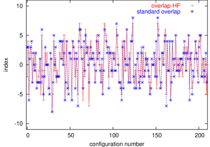
Figure 34: Index histories for $D_{\rm ovHF}$ (see Section 7) and for the standard overlap operator $D_{\rm N}$ (at $\rho=1.6$) for the same set of QCD configurations.

Nevertheless both follow well the expected Gaussian distributions $\propto\exp(-{\rm const.}\cdot\nu^{2})$, with a width $\approx 3.3$, see Figure 35.

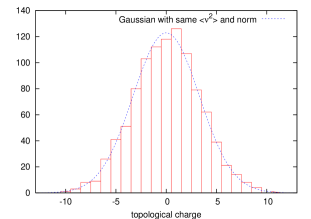
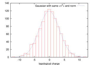
Figure 35: The histogram of $D_{\rm ovHF}$ indices (on the left) and of $D_{\rm N}$ indices (on the right), on a $12^{3}\times 24$ lattice at $\beta=5.85$. In both cases, 1013 configurations are included [104].

This width fixes the topological susceptibility (cf. eq. (2.15))

$$\chi_{\rm top}=\frac{1}{V}\langle\nu^{2}\rangle\ ,$$ (8.18)

which is of importance to explain the heavy mass of the $\eta^{\prime}$-meson [142].

In Figure 36 we present our results with $D_{\rm ovHF}$ and $D_{\rm N}$ on the lattice referred to so far, plus a result for $D_{\rm N}$ at $\beta=6$ in the same physical volume (lattice size $16^{3}\times 32$). We also mark the continuum extrapolation according to Ref. [143], which is fully consistent with our results. That measurement of $\chi_{\rm top}$ was based on $D_{\rm N}$ indices on $L^{4}$ lattices. The resulting value for $\chi_{\rm top}$ is compatible with the Witten-Veneziano scenario that much of the $\eta^{\prime}$ mass is generated by a $U(1)$ anomaly [142].

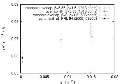
Figure 36: The topological susceptibility measured by indices of $D_{\rm ovHF}$ and of $D_{\rm N}$, in a volume $V=(1.48~{}{\rm fm})^{3}\times 2.96~{}{\rm fm}$, with two different lattice spacings $a$. Our data — given in detail in Ref. [104] — agree well with the continuum extrapolation in Ref. [143].

8.4 The $\epsilon$-regime

We first repeat that the $\epsilon$-regime of QCD is characterised by a relatively small volume, i.e. the correlation length $\xi$ exceeds the linear box size $L$. Together with the requirement (8.6) this amounts to the condition

$$\frac{1}{m_{\pi}}>L\gg\frac{1}{4\pi F_{\pi}}\ .$$ (8.19)

In such a box, the $p$-expansion of $\chi$PT fails, in particular because of the importance of the zero modes. However, the latter can be treated separately by means of collective variables, and the higher modes — along with the pion mass — are then captured by the $\epsilon$-expansion [123]. One now counts the ratios

$$\frac{m_{\pi}}{\Lambda_{\rm QCD}}\sim\frac{p^{2}}{\Lambda_{\rm QCD}^{2}}\sim\frac{1}{(LF_{\pi})^{2}}$$ (8.20)

as small quantities in the same order.

This setting, where pions are squeezed into a tiny box, cannot be considered physical. Nevertheless there is a strong motivation for its numerical study: the point is that the finite size effects are parametrised by the LECs of the effective chiral Lagrangian as they occur in infinite volume. Hence the physical values of the LECs can (in principle) be evaluated even in such an unphysically small box, as we mentioned in the introduction to Section 8.

Unfortunately, most results for the LECs in the $\epsilon$-regime are obtained in the quenched approximation so far, hence they are affected by (mostly logarithmic) finite size effects [144]. So the final results by this method still have to wait for the feasibility of QCD simulations with dynamical, chiral quarks. These prospects will be commented on in Subsection 9.2.

8.4.1 A 3-loop calculation in the $\epsilon$-expansion

The chiral symmetry breaking for two flavours is locally isomorphic to orthogonal groups,

$$SU(2)\otimes SU(2)\to SU(2)\quad\sim\quad O(4)\to O(3)\ .$$ (8.21)

Generally, the spontaneous symmetry breaking $O(N)\to O(N-1)$ generates $N-1$ NGBs. They can be described by the non-linear $\sigma$-model and studied with the formalism of $\chi$PT. In $d=3$ and $d=4$ the corresponding Lagrangian involves an infinite string of terms, which can be ordered by the power of the momenta involved. In a volume $V=L^{d}$ (with periodic boundary conditions) we count the momenta as $\partial_{\mu}=O(L^{-1})$, and we obtain the leading terms

$${\cal L}^{\rm(sym)}[\vec{S}] = \frac{F^{2}}{2}\partial_{\mu}\vec{S}\partial_{\mu}\vec{S}+\frac{1}{2}g_{4}^{(1)}\partial^{2}\vec{S}\partial^{2}\vec{S}+\frac{1}{4}g_{4}^{(2)}(\partial_{\mu}\vec{S}\partial_{\mu}\vec{S})^{2}$$ (8.22)

$$+ \frac{1}{4}g_{4}^{(3)}(\partial_{\mu}\vec{S}\partial_{\nu}\vec{S})^{2}+O(L^{-6})\ ,\qquad\vec{S}^{\,2}(x)\equiv 1\ ,\quad$$

where we attach an independent LEC to each term. We may also add terms that break the $O(N)$ symmetry explicitly through a small, constant magnetic field $\vec{H}$, which adopts the rôle of the light quark masses,

$$-{\cal L}^{\rm(sb)}[\vec{S}] = \Sigma(\vec{H}\vec{S})+h_{2,0}^{(1)}(\vec{H}\vec{S})^{2}+h_{2,0}^{(2)}(\vec{H}\vec{H})^{2}$$ (8.23)

$$+ h_{1,2}^{(1)}(\vec{H}\vec{S})\,(\partial_{\mu}\vec{S}\partial_{\mu}\vec{S})+h_{1,2}^{(2)}(\vec{H}\partial^{2}\vec{S})+\dots\quad.$$

Then we assemble the total Lagrangian ${\cal L}={\cal L}^{\rm(sym)}+{\cal L}^{\rm(sb)}$.

We count $H:=|\vec{H}|=O(V^{-1})$, so that the NGBs with $m^{2}=\Sigma H/F^{2}$ feel the finite size strongly, $mL\ll 1$. Then the partition function can be $\epsilon$-expanded in the dimensionless ratio $\epsilon=L^{2-d}/F^{2}$ in $d=3$ and $4$.

To compute the free energy ${\cal F}=-\ln Z$ one first has to find a way to handle the zero modes. We mentioned before that this can be achieved by using collective variable [123]. In the present case, one considers the magnetisation

$$\vec{M}:=\int d^{d}x\,\vec{S}(x)=|\vec{M}|\,\Omega\,\vec{e}\ ,$$ (8.24)

where $\vec{e}=\vec{H}/|\vec{H}|$ is a fixed unit vector and $\Omega\in O(N)$ is integrated over in the functional integral. (The corresponding unitary integration for quark flavours is discussed in Refs. [145].) Here the vector field $\vec{S}$ can be decomposed into one dominant component plus fluctuations ${\underline{\pi}}(x)=(\pi_{1}(x),\dots\pi_{N-1}(x))$, $\ \pi_{i}(x)=O(L^{1-d/2})$, which are treated perturbatively. In this way, the partition function can be evaluated order by order.

This was first carried out to 2 loops in Ref. [126], where the functional measure was treated with the Faddeev-Popov procedure (the constraint $\delta(\vec{S}^{\,2}-1)$ is implemented in an exponential form). A different method was applied in Ref. [146], which was based on the Polyakov measure [147]. That measure was originally introduced in the framework of string theory and it captures the above constraint by integrating ${\cal D}{\underline{\pi}}$ over the $\epsilon$-expanded elements of a metrics in flavour space. In this way we computed the partition function to 3 loops. In both cases dimensional regularisation [34] was used. It turned out that the free energy is in fact perturbatively renormalisable order by order (although the number of required counter terms increases rapidly in each order). This property is highly non-trivial due to the requirement that the renormalised LECs must not pick up any volume dependence. This is realised both, in $d=3$ and in $d=4$, for the large number of terms occurring to the 3-loop order, thanks to numerous cancellations between forbidden contributions. These calculations represent therefore a sensitive test for the validity of the $\epsilon$-expansion scheme, as well as the methods used for the treatment of the functional measure.

Before chiral lattice fermions became available, the program of evaluating LECs through simulations in the $\epsilon$-regime was tested in the framework of this spin model [148].

8.4.2 The chiral condensate

Chiral Random Matrix Theory (RMT) conjectures predictions for the low lying eigenvalues, ordered as $\lambda_{n}$, $n=1,2,3\dots$ (excluding possible zero eigenvalues) of the Dirac operator in the $\epsilon$-regime; for a review, see Ref. [149]. More precisely, it conjectures densities of the dimensionless variables $\Sigma V\lambda_{n}$, where $\Sigma$ is the chiral condensate in the effective Lagrangian (8.5). Here we focus on the variable $z:=\Sigma V\lambda_{1,P}$, where $\lambda_{1,P}$ emerges from the leading non-zero eigenvalue $\lambda_{1}$ if the spectral circle of the overlap operator is mapped stereographically onto the imaginary axis, $\lambda_{1,P}=|\lambda_{1}/(1-\lambda_{1}/2\rho)|$.

These RMT predictions depend on $|\nu|$, the absolute value of the topological charge. Here we make use of the explicit formulae [150] for the density of the first non-zero (re-scaled) eigenvalues $z$ in the sectors $|\nu|$, which we denote by $\rho_{1}^{(|\nu|)}(z)$. For the lowest eigenvalues, the particular density $\rho_{1}^{(0)}$ was first confirmed by staggered fermion simulations (results are summarised in Ref. [149]). But in those studies the charged sectors yielded the very same density, in contradiction to RMT.

The distinction between the topological sectors was first observed to hold for $D_{\rm N}$, following the RMT predictions to a good precision [152], if the linear box size exceeds a lower limit of about $L\mathop{\raise 1.29167pt\hbox{$>$\kern-7.5pt\raise-4.73611pt\hbox{$\sim$}}}1.1~{}{\rm fm}$ (the exact limit depends on the criterion, of course). The predictions for the densities of the leading non-zero eigenvalues in the sectors $|\nu|=0,\ 1$ and $2$ are shown in Figure 37 on the left; we see that zero modes repel the finite eigenvalues. On the right-hand-side of Figure 37 we present results for the corresponding cumulative density with $D_{\rm N}$ on a $10^{4}$ lattice at $\beta=5.85$ (box length $\simeq 1.23~{}{\rm fm}$).

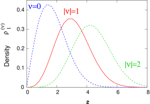
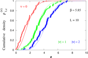
Figure 37: On the left: RMT predictions for the leading non-zero Dirac eigenvalue in the topological sectors with charge $|\nu|=0,\ 1$ and $2$.
On the right: RMT predictions (lines) and simulation results for the corresponding cumulative densities. The numerical data were obtained with $D_{\rm N}$ on a $10^{4}$ lattice at $\beta=5.85$ (see first work in Ref. [152]), and they do essentially follow the RMT predictions. The confidence level for the agreement of cumulative densities has been verified with the Kolmogorov-Smirnov test [109].

Once the predicted densities $\rho_{1}^{(|\nu|)}$ (marked by lines) are well reproduced, we can read off the value of $\Sigma$, which is the only free fitting parameter for all topological sectors. We proceed to larger lattices and show our result for $D_{\rm ovHF}$ on a $12^{3}\times 24$ lattice at $\beta=5.85$ in Figure 38 [104]. The optimal fit shown in this plot, and its counterpart for the Neuberger operator $D_{\rm N}$, yield

$$\Sigma^{1/3}=298(4)~{}{\rm MeV}\quad({\rm from}~{}D_{\rm ovHF})\ ,\ \Sigma^{1/3}=301(4)~{}{\rm MeV}\quad({\rm from}~{}D_{\rm N})\ .$$ (8.25)

These fits focus on the lowest eigenvalues resp. energies, where chiral RMT is most reliable. Clearly, in this range the neutral sector ($\nu=0$) dominates. In the case of $D_{\rm N}\,$, the charged sectors $|\nu|=1$ and $2$ alone would favour a different $\Sigma$ value [104]. Such ambiguities are quite strong in the results with smeared staggered fermions [153]. In the case of $D_{\rm ovHF}$, however, a unique $\Sigma$ works well for all the three sectors $|\nu|=0,1,2$, up to about $z\approx 3$, as Figure 38 shows. This range extends well beyond the Thouless value $z_{\rm Thouless}=F_{\pi}^{2}\sqrt{V}\mathop{\raise 1.29167pt\hbox{$<$\kern-7.5pt\raise-4.73611pt\hbox{$\sim$}}}1$, which is often understood as a threshold for the RMT applicability.

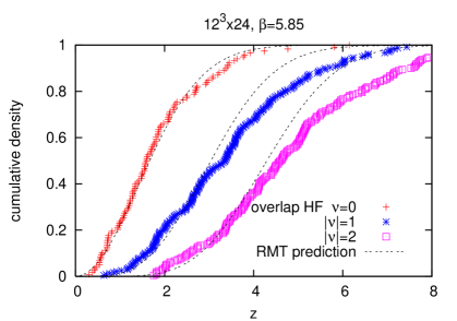
Figure 38: The cumulative density of the (Möbius projected) lowest Dirac eigenvalue $\lambda_{1,P}$ of the overlap-HF operator, in the topological sectors $|\nu|=0$, $1$ and $2$. We compare the chiral RMT predictions to our data for $z=\Sigma V\lambda_{1,P}$ with $\Sigma^{1/3}=298~{}{\rm MeV}$ — the optimal value in the neutral sector ($\nu=0$). This value works well up to $z\approx 3$ for all topological sectors, i.e. well beyond the Thouless value $z_{\rm Thouless}\mathop{\raise 1.29167pt\hbox{$<$\kern-7.5pt\raise-4.73611pt\hbox{$\sim$}}}1$, which is often considered a theoretical bound for the applicability of these predictions.

As an alternative approach to test the agreement of our data with the chiral RMT, and to extract a value for $\Sigma$, we now consider the mean values of the leading non-zero Dirac eigenvalues $\lambda_{1}$ in all the charge sectors up to $|\nu|=5$. In physical units, the results $\langle\lambda_{1,P}\rangle$ agree very well for different overlap operators and lattice spacings — see Figure 39 — although this consideration extends beyond very low energy. Each single result for $\langle\lambda_{1,P}\rangle_{|\nu|}$ can then be matched to the RMT value for a specific choice of $\Sigma$. It is very remarkable that all these 18 results are compatible with RMT if we choose

$$\Sigma=(290(6)~{}{\rm MeV})^{3}\ ,$$ (8.26)

as Figure 39 also shows.

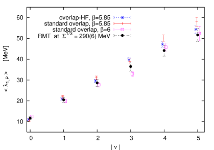
Figure 39: The mean values of the first non-zero Dirac eigenvalue (in physical units) in the charge sectors $|\nu|=0\dots 5$. All these numerical results [104] agree with chiral RMT if we choose $\Sigma^{1/3}=290(6)~{}{\rm MeV}$.

A renormalisation procedure for $\Sigma$ obtained in this way is discussed in Ref. [154]. However, we will only use this quenched lattice result as a fitting input in Subsection 8.4.3, so we stay with the bare condensate $\Sigma$ for our fixed lattice parameters.
We add that there are also first applications of this technique with dynamical overlap fermions [155].

8.4.3 The pion decay constant determined from the axial current correlator

In order to relate our quenched simulation results to the effective low energy theory, we now refer to quenched $\chi$PT. In that framework, mesonic correlation functions were calculated to the first order in Refs. [156, 157]. The vector current correlation function vanishes, while the scalar and pseudoscalar correlators involve already in the first order additional, quenching specific LECs, which obstruct the access to the physical LECs in the Lagrangian (8.5). Therefore we first focus on the axial-vector correlator, which only depends on $\Sigma$ and $F_{\pi}$ in the first order. In particular we are going to compare our data to the quenched $\chi$PT prediction in a (periodic) volume $V=L^{3}\times T$ [157], for the topological sectors with charge $\pm\nu$,

$$Z_{A}^{2}\cdot\langle A_{4}(t)\,A_{4}(0)\rangle_{|\nu|} = 2\left(\frac{F_{\pi}^{2}}{T}+2m_{q}\,\Sigma_{|\nu|}(z_{q})\,T\,h_{1}(\tau)\right)\ ,$$ (8.27)

$$h_{1}(\tau) = \frac{1}{2}\Big{(}\tau^{2}-\tau+\frac{1}{6}\Big{)}\ ,\qquad\tau=\frac{t}{T}\ ,$$

$$\Sigma_{\nu}(z_{q}) = \Sigma\left(z_{q}\Big{[}I_{\nu}(z_{q})K_{\nu}(z_{q})+I_{\nu+1}(z_{q})K_{\nu-1}(z_{q})\Big{]}+\frac{\nu}{z_{q}}\right)\ ,$$

where

$$A_{4}(t)=a^{3}\sum_{\vec{x}}\bar{\psi}(t,\vec{x})\gamma_{5}\gamma_{4}\psi(t,\vec{x})\qquad\quad(t>0)$$ (8.28)

is the bare axial-vector current at 3-momentum $\vec{p}=\vec{0}$. $I_{\nu}$ and $K_{\nu}$ are modified Bessel functions, and $z_{q}:=\Sigma Vm_{q}$ (in analogy to the dimensionless variable $z$ in Subsection 8.4.2).

It is remarkable that this prediction in the $\epsilon$-regime has the shape of a parabola with a minimum at $t=T/2$. This is in qualitative contrast to the ${\tt cosh}$ behaviour, which is standard in large volumes. $\Sigma$ affects both, the curvature and the minimum of this parabola, whereas $F_{\pi}$ only appears in the additive constant — that feature is helpful for its evaluation.

A first comparison of this curve to lattice data was presented in Ref. [158], using $D_{\rm N}$ at $\beta=6$, $\rho=1.4$, $am_{q}=0.01$ on lattice sizes $10^{3}\times 24$ and $12^{4}$. For the anisotropic volume the linear size of $L\simeq 0.93~{}{\rm fm}$ turned out to be too small: the data for $\,\langle A_{4}(t)\,A_{4}(0)\rangle_{1,2}\,$ were incompatible with the parabola of eq. (8.27) for any positive $\Sigma$. This observation is consistent with the lower bound for $L$ that we also found for the agreement of the microscopic spectrum with chiral RMT ($L\mathop{\raise 1.29167pt\hbox{$>$\kern-7.5pt\raise-4.73611pt\hbox{$\sim$}}}1.1~{}{\rm fm}$, see Subsection 8.4.3).

Another observation in that study was that the corresponding Monte Carlo history in $\nu=0$ is plagued by strong spikes, giving rise to large statistical errors. A huge statistics of $O(10^{4})$ topologically neutral configurations would be required for conclusive results. These spikes occur for the configurations with a tiny (non-zero) Dirac eigenvalue $\lambda_{1,P}$. It agrees again with chiral RMT that such configurations are most frequent in the topologically neutral sector, see Figure 37. (A method called “low mode averaging” was designed and applied to alleviate this problem [159].)

However, without applying that method we obtained a decent agreement with the prediction (8.27) in the $12^{4}$ lattice mentioned above ($V\simeq(1.12~{}{\rm fm})^{4}$) in the sector $|\nu|=1$ [158]. In view of the leading LECs, it seems unfortunately impossible to extract a value of $\Sigma$ from such data (although it is encoded in $z_{q}$), since the theoretical curvature depends on it only in an extremely weak way. On the other hand, $F_{\pi}$ can be extracted quite well from the vicinity of the minimum at $t=T/2$, but the value found in Ref. [158] was too large.

Next a study of that kind appeared in Ref. [133], which also used $D_{\rm N}$, at $\beta=5.85$ (and $\rho=1.6$), now on a $10^{3}\times 20$ lattice. This work analysed the sectors $|\nu|=0$ and 1. As a reason for this limitation the authors referred to the condition $|\nu|\ll\langle\nu^{2}\rangle$. As we mentioned in Subsection 8.4.2, one expects $\langle\nu^{2}\rangle\propto V$ (up to artifacts), see eq. (8.18), hence this limitation was imposed by the volume.

In Ref. [104] we presented again results at $\beta=5.85$ on a $12^{3}\times 24$ lattice, where the volume admits $|\nu|=2$. We measured for both, $D_{\rm ovHF}$ and $D_{\rm N}$, the axial-vector correlators at the masses $am_{q}=0.001$, $0.003$ and $0.005$, which are safely in the $\epsilon$-regime. We fitted the data to eq. (8.27) by inserting the chirally extrapolated factors $Z_{A}$ ($1.17$ for $D_{\rm ovHF}$ [104] and $1.45$ for $D_{\rm N}$ [130], see Subsection 8.2), along with the $\Sigma$ values in eq. (8.25). For each of the overlap operators we performed — at each of the quark masses — a global fit over the topological sectors that we considered. The result for $D_{\rm ovHF}$ is shown in Figure 40. It revealed for the first time a convincing distinction between the sectors $|\nu|=1$ and $|\nu|=2$ — this predicted topological splitting could not be observed for $D_{\rm N}$ up to now. For $D_{\rm N}$ at $am_{q}=0.005$ we also include the neutral sector; as expected it has clearly larger errors than the charged sectors, but it is helpful nevertheless to reduce the error on $F_{\pi}$ in the global fit. The values for $F_{\pi}$ obtained in this way for $D_{\rm ovHF}$ and for $D_{\rm N}$ are in accurate agreement, as Table 2 shows.

$am_{q}$	$D_{\rm ovHF}$	$D_{\rm N}$
$0.001$	$F_{\pi}=(110\pm 8)~{}{\rm MeV}$	$F_{\pi}=(109\pm 11)~{}{\rm MeV}$
$0.003$	$F_{\pi}=(113\pm 7)~{}{\rm MeV}$	$F_{\pi}=(110\pm 11)~{}{\rm MeV}$
$0.005$	$F_{\pi}=(115\pm 6)~{}{\rm MeV}$	$F_{\pi}=(111\pm 4)~{}{\rm MeV}$

Table 2: Our results for the pion decay constant $F_{\pi}$, evaluated in the $\epsilon$-regime based on the axial-current correlation function (8.27). These results are obtained at $\beta=5.85$ on a $12^{3}\times 24$ lattice. The statistics involved $100$ propagators for $D_{\rm N}$ at $am_{q}=0.005$, and $50$ propagators in all other cases. $F_{\pi}$ was determined from fits to the quenched $\chi$PT formula (8.27) in the range  $t/a\in[11,13]$.

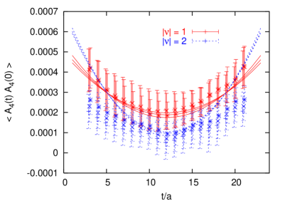
Figure 40: Lattice data obtained with $D_{\rm ovHF}$ for the axial-current correlation functions, measured separately in the topological sectors $|\nu|=1$ and $2$. The curves are global fits (over both sectors) to the quenched $\chi$PT formula (8.27), for each of our three masses in the $\epsilon$-regime. They single out the values of $F_{\pi}$ given in Table 2.

8.4.4 The pion decay constant based on the zero modes

At last we review our results based on an alternative method to evaluate $F_{\pi}$ in the $\epsilon$-regime [104]. This method was introduced in Ref. [160], and it involves solely the zero mode contributions to the pseudoscalar correlation function. Here one works directly in the chiral limit. Let us briefly summarise the main idea of this approach.

Ref. [160] computed the chiral Lagrangian to the next-to-next-to-leading order in quenched $\chi$PT, ${\cal L}_{\rm q\chi PT}^{(2)}$. It can be written in a form that involves an auxiliary scalar field $\Phi_{0}$, which is coupled to the quasi Nambu-Goldstone field $U$ by a new LEC denoted as $K$. The auxiliary field also contributes

$${\cal L}^{(2)}[\Phi_{0}]=\frac{\alpha_{0}}{2N_{c}}\partial_{\mu}\Phi_{0}\partial_{\mu}\Phi_{0}+\frac{m_{0}^{2}}{2N_{c}}\Phi_{0}^{2}$$ (8.29)

to ${\cal L}_{\rm q\chi PT}^{(2)}$, which brings in $\alpha_{0}$ and $m_{0}$ as another two quenching specific LECs, in addition to $K$. The field $\Phi_{0}$ supplements the quenching effects; in the dynamical case it decouples form the field $U$.

It is ambiguous how to count these additional terms in the quenched $\epsilon$-expansion. Ref. [160] assumes the action terms with the coefficients $\alpha_{0}$ and $\,K\sqrt{N_{c}}\,$ to be of $O(1)$, whereas the one with $m_{0}$ is in $O(\epsilon)$. The last assumption is somewhat unusual (for instance, it differs from the framework of Subsection 8.5.1). Nevertheless it is an acceptable possibility, which simplifies this approach since it removes the auxiliary mass term from the dominant order. If one further defines the dimensionless parameter

$$\alpha:=\alpha_{0}-\frac{4N_{c}^{2}KF_{\pi}}{\Sigma}\ ,$$ (8.30)

then only the LECs $F_{\pi}$ and $\alpha$ occur in this order.

For $N_{f}$ valence quark flavours, this approach considers the correlation function of the pseudoscalar density $P(x)$ (defined in Subsection 8.2), which is decomposed into a connected plus a disconnected part. In a spectral decomposition of the propagators one obtains the residuum in terms of the zero modes,

$${}^{~{}\lim}_{m_{q}\to 0}\ (m_{q}V)^{2}\langle P(x)P(0)\rangle_{\nu} = N_{f}C^{(1)}_{|\nu|}(x)+N_{f}^{2}C^{(2)}_{|\nu|}(x)$$

$${\rm connected:~{}~{}~{}}C^{(1)}_{|\nu|}(x) = -\langle v_{j}^{\dagger}(x)v_{k}(x)\cdot v_{k}^{\dagger}(0)v_{j}(0)\rangle_{|\nu|}$$

$${\rm disconnected:~{}~{}~{}}C^{(2)}_{|\nu|}(x) = \langle v_{j}^{\dagger}(x)v_{j}(x)\cdot v_{k}^{\dagger}(0)v_{k}(0)\rangle_{|\nu|}\ .$$ (8.31)

The vectors $v_{j}$ denote the (exact) zero modes of the Ginsparg-Wilson operator at $m_{q}=0$. In the terms for $C^{(i)}_{|\nu|}$ these zero modes are summed over.

Next we consider the spatial integral $\int d^{3}x\,P(x)P(0)$. Now the above procedure for the correlation function leads to functions $C^{(i)}_{|\nu|}(t)$, $i=1,2$, which are given explicitly in Ref. [160]. In principle, these functions could be measured and fitted to the predictions in order to determine $F_{\pi}$ and $\alpha$. In practice, however, it is much more promising to consider just the leading term in the expansion at $t=T/2$,

$$\frac{V}{L^{2}}\frac{d}{dt}C^{(i)}_{|\nu|}(t)|_{t=T/2}=D^{(i)}_{|\nu|}s+O(s^{3})\ ,\quad s=t-\frac{T}{2}\ ,\quad i=1,2\ .$$ (8.32)

The explicit slope functions $D^{(i)}_{|\nu|}$ in a volume $V=L^{3}\times T$ are given in Refs. [160, 103, 104]. (They also involve a shape coefficient, which we computed for our anisotropic volume according to the prescription in Ref. [126].)

We evaluated the LECs $F_{\pi}$ and $\alpha$ from fits to the linear term in eq. (8.32). For each of our lattice sizes and for each type of overlap operator we performed a global fit over the topological sectors $|\nu|=1$ and $2$, in a fitting range $s_{\rm max}\,$. The slopes tend to be stable over a variety of fitting ranges $s\in[-s_{\rm max},s_{\rm max}]$, $s_{\rm max}=a,\,2a,\,3a\dots$. The deduced optimal values for $F_{\pi}$ are shown in Figures 41, and the values for $F_{\pi}$ and $\alpha$ at $s_{\rm max}/a=1$ are given in Table 3. We see that the results for different lattice spacings and overlap Dirac operators are in good agreement. Considering also $\alpha(s_{\rm max})$, we found the most stable plateau for $D_{\rm ovHF}$ [104].

Dirac operator	$D_{\rm ovHF}$	$D_{\rm N}$	$D_{\rm N}$
$\beta$	$5.85$	$5.85$	$6$
lattice size	$12^{3}\times 24$	$12^{3}\times 24$	$16^{3}\times 32$
$F_{\pi}$	$(80\pm 14)$ MeV	$(74\pm 11)$ MeV	$(75\pm 24)$ MeV
$\alpha$	$-17\pm 10$	$-19\pm 8$	$-21\pm 15$

Table 3: Our results in the $\epsilon$-regime for the pion decay constant $F_{\pi}$ — along with the quenching specific LEC $\alpha$ given in eq. (8.30) — based on the zero mode contributions to the pseudoscalar correlation function. We give results for the fitting range $s_{\rm max}=a$, which is most adequate in the light of eq. (8.32).

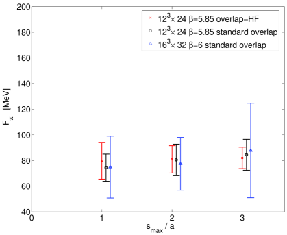
Figure 41: The results for $F_{\pi}$ based on a global fit of our data to a quenched $\chi$PT prediction for the zero mode contributions to the pseudoscalar correlations function. We show the $F_{\pi}$ results of a two parameter fit (for $F_{\pi}$ and $\alpha$) over the ranges $s\in[T/2-s_{\rm max},T/2+s_{\rm max}]$.

The values that we now obtain for $F_{\pi}$ is below those of Section 8.4.3, which used a different observable and a different $\epsilon$-counting rule for the quenched terms. In fact, the $F_{\pi}$ results in Table 3 are close to the phenomenological value (the latter is shifted down to $\approx 86~{}{\rm MeV}$ if one extrapolates to the chiral limit [161]). Our values for $F_{\pi}$ and $\alpha$ obtained from the zero modes are somewhat below the values reported in Ref. [160] based on the same method. We suspect that the anisotropic shape of our volumes, $T=2L$, could be the main source of this deviation [162].

9 Epilogue

The central concept in this work are block variable RGTs (renormalisation group transformations) applied to lattice regularised quantum field theories. We described this method for various types of field theoretic models, and focused in particular on the limit obtained under iterated RGTs. This leads to lattice formulations with fascinating properties: in particular the symmetries and the scaling quantities of the continuum theories can — in principle — be reproduced exactly on the lattice. This amazing feature also includes exact supersymmetry and precise topological sectors on the lattice. The corresponding perfect lattice actions were constructed explicitly for the case of free particle. For interacting fields this can in general only be achieved approximately (as an exception we considered the Gross-Neveu model in the large $N$ limit). We discussed perturbatively perfect actions in various models, as well as issues of truncation, parameterisation and gauging. We also demonstrated that different kinds of anomalies are represented correctly in this way.

We summarised a variety of simulation results based on such approximately perfect actions. They reveal a number of properties which are superior to the standard lattice formulations, in particular an improved symmetry and scaling behaviour. The chiral symmetry of massless fermions can be rendered exact by means of the overlap formula. This provides a lattice formulation, which performs very well in toy model simulations, and it is currently being applied to QCD.

9.1 The status of overlap-HF applications in QCD with light quarks

In Section 7 we reviewed our construction of overlap hypercube Dirac operators $D_{\rm ovHF}$, which are especially suitable at lattice spacings of $a\simeq 0.093~{}{\rm fm}$ and $a\simeq 0.123~{}{\rm fm}$. In both cases, they display a strongly improved locality compared to the standard overlap operator $D_{\rm N}$. Hence $D_{\rm ovHF}$ defines chiral fermions on coarser lattices.

Section 8 summarised quenched simulations with $D_{\rm ovHF}$ and with $D_{\rm N}$ in a volume $V\simeq(1.48~{}{\rm fm})^{3}\times(2.96~{}{\rm fm})$ at $\beta=5.85$ and at $\beta=6$.

Subsection 8.2 dealt with the $p$-regime, where we measured the meson masses $m_{\pi}$ and $m_{\rho}$ (though only the former was presented here, for $m_{\rho}$ we refer to Ref. [104]), the quark mass $m_{\rm PCAC}$ (based on the axial Ward identity) and the pion decay constant $F_{\pi}$ at bare quark masses ranging from $16.1~{}{\rm MeV}$ to $161~{}{\rm MeV}$. The results for $m_{\pi}$ and $m_{\rho}$ are similar for $D_{\rm ovHF}$ and $D_{\rm N}$. On the other hand, for $D_{\rm ovHF}$ the quark mass $m_{\rm PCAC}$ is much closer to $m_{q}$ than in the standard overlap formulation. This implies $Z_{A}\approx 1$, which is favourable for the connection to perturbation theory. Regarding $F_{\pi}$, it turned out that the data obtained in the $p$-regime can hardly be extrapolated to the chiral limit.

In Subsection 8.3 we discussed a way to stabilise the topological sector in a Monte Carlo history. We also considered the distribution of a large number of topological charges defined by the fermion indices of $D_{\rm ovHF}$ or of $D_{\rm N}$. We found histograms which approximate well a Gaussian distribution, consistent with the conservation of parity invariance. The resulting topological susceptibility is in good agreement with the literature, and with the Witten-Veneziano scenario.

In Subsections 8.4 we proceeded to the $\epsilon$-regime, where we first summarised a 3-loop calculation in the framework of the $\epsilon$-expansion. Numerically we determined a value for the chiral condensate from the distribution of the lowest eigenvalues. For both, $D_{\rm ovHF}$ and $D_{\rm N}$ we identified $\Sigma$ close to $(300~{}{\rm MeV})^{3}$.

We evaluated $F_{\pi}$ in the $\epsilon$-regime in two ways, from the axial-current correlation and from the zero mode contributions to the correlation of the pseudoscalar density. These two methods handle the $\epsilon$-counting of the quenched terms differently, and they yield different values for $F_{\pi}$. The axial-current method leads to $F_{\pi}\approx 110~{}{\rm MeV}$, which is consistent with part of the quenched results in the literature. The zero mode method leads to a lower $F_{\pi}$, in the vicinity of the phenomenological value. The result of Ref. [159] — empolying yet another method, based on the $\Delta I=1/2$ rule, still in the $\epsilon$-regime — is in between.

From the current results we conclude that the methods applied here do have the potential to evaluate at least the leading LECs from lattice simulations in the $\epsilon$-regime. The quenched data match the analytical predictions qualitatively (if the volume is not too small) and — in the setting we considered — they lead to results in the magnitude of the LECs in Nature. However, the quenched results are volume dependent and in addition ambiguous: different methods yield different values.

For values that can be confronted with phenomenology in detail, simulations with dynamical quarks will be needed. In particular the $\epsilon$-regime requires then dynamical Ginsparg-Wilson fermions. This regime is promising in view of the lattice size. Also the option to extract physical information from single topological sectors is attractive, since it is very difficult to change the sector frequently in the course of Hybrid Monte Carlo histories. The question is if one is able to handle sufficiently small quark masses in dynamical simulations.

9.2 Prospects for dynamical simulations with chiral fermions

We just pointed out that the results for light quarks can be linked successfully to $\chi$PT (Chiral Perturbation Theory), but to some extent they are obstructed up to now by the quenched approximation. Quenching has been necessary so far in QCD simulations with chiral quarks due to limitations in the computational resources.

We hope to overcome this limitation — and the systematic errors that it causes — in the foreseeable future, and to be able to proceed to simulations with dynamical chiral quarks. However, in addition to powerful machines this step also requires new algorithmic tools, which are currently under consideration. Also in this respect overlap-HFs open up new perspectives.

Due to the similarity with the hypercubic kernel, a low polynomial of this kernel can be used as a numerically cheap way to evaluate the fermionic force in the Hybrid Monte Carlo (HMC, [78]) algorithm. This approach is conceptually guided by the algorithm that we used for the simulation of quasi-perfect staggered fermions (see Ref. [77] and Subsection 6.3.2). Also for the overlap-HF formulations of Ref. [75] it is under investigation in the two-flavour Schwinger model. First the extreme case of using directly $D_{\rm HF}$ in the force term was studied in Ref. [163], which reported a decreasing acceptance rate for an increasing volume. However, it turned out that the acceptance rate can be improved by an order of magnitude by correcting the fermionic force term at least to a low accuracy like $0.005$, which allows for efficient HMC simulations with very light (degenerate) overlap-HFs [164]. Of course, the overlap operator has be to very precise in the Metropolis accept/reject step (we set it to $10^{-16}$). We verified the acceptance rate as well as algorithmic requirements, namely area conservation and reversibility.

In our simulations at $\beta=5$ on a $16\times 16$ lattice [164] (with the plaquette gauge action) we confirmed the similarity between the kernel and the overlap operator by considering the spectra, and we observed a high level of locality for this formulation. The characteristic decay hardly changes in the fermion mass range $0.03\dots 0.24$, and the locality is by far superior to the standard overlap operator. As an observable we evaluate the chiral condensate at light fermion masses, based on the ratio between low lying Dirac eigenvalues in different topological sectors (the relevant formulae were taken from Ref. [165]). This represents one of the first measurements with dynamical overlap fermions. Our results for the chiral condensate at various masses are in excellent agreement with analytic predictions, which were obtained with bosonisation and low energy approximations [166].

In QCD, simulations with dynamical overlap fermions are still in an early stage; for recent status reports we refer to Refs. [167]. Regarding the approximately chiral fermion formulations explained in this work, dynamical HFs are currently investigated, and interesting results for their phase diagram are available already [169]. It provides access to a mass ratio $m_{\pi}/m_{\rho}\leq 0.8$ at the thermal crossover, which is not the case for Wilson fermions. In this context we add that the truncated classically perfect action of Ref. [14], and the “chirally improved” formulation of Refs. [101], are currently applied in dynamical simulations as well [170].

Also the topology conserving gauge actions — that we discussed in Subsection 8.3 — appears to be helpful in simulations with dynamical quarks due to the suppression of small plaquette value, as suggested in Ref. [138] and tested in Ref. [140].

The quenched studies reported here show that we have methods at hand, which are applicable for instance for the evaluation of Low Energy Constants in the chiral Lagrangian from first principles. These constants play a prominent rôle in QCD at low energy, hence their determination is a major challenge and a sensitive test for QCD, to be addressed with dynamical Ginsparg-Wilson fermions.

10 Further Fields of Research

In my diploma thesis I investigated mathematical and mechanical models for certain brain activities and the resulting neural signals. More precisely, I analysed numerically and analytically the time evolution of jerky eye motions and the required coordination of nerve signals, particularly in view of the non-Abelian dynamics.

For short periods I was involved in two experiments at CERN that observed the electroweak mixing angle (CHARM II) and neutral kaon decays (CP-LEAR).

In a work with J.J. Giambiagi we discussed solutions of the spherically symmetric wave equation and Klein-Gordon equation in an arbitrary real number of spatial and temporal dimensions [171]. Starting from a given solution, we presented various procedures to generate further solutions in the same or in different dimensions. The transition from odd to even or non-integer dimensions could be performed by fractional derivation or integration. We also discussed the analytic continuation to arbitrary real powers of the D’Alembert operator. Finally we worked out operators which transform a time into a space coordinate and vice versa, and we commented on a possible application to black holes.

In a completely different project we addressed statistical mechanics and investigated the phase diagram of the 2d O(3) lattice model with a $\theta$-term [172]. The simulation made use of the Wolff cluster algorithm [173] and required the construction of an improved estimator, which could only be achieved by a new method. The clusters carry half integer topological charge and most of the charged clusters can be identified with merons. We confirmed to a high accuracy the prediction by I. Affleck et al. [174], who expected a second order phase transition at $\theta=\pi$ due to analogies to Haldane’s conjecture about quantum spin chains [175]. The traditional picture explains this phase transition by the neutralisation of vortex-antivortex pairs. In the framework of our “meron cluster algorithm”, this picture could be formulated precisely, without breaking the O(3) symmetry.

Further algorithmic elements were added in Ref. [176]. Recently another meron cluster simulation was performed successfully for the $XY$ spin chain [18].

For a few years, I have been working in a collaboration which studied large $N$ reduced matrix models as candidates for a non-perturbative formulation of string theory. In particular, we have simulated variants of the so-called IKKT model (or IIB matrix model) [177], which corresponds to a dimensional reduction of super Yang-Mills theory to zero dimensions. This model is formulated in 10 (target) dimensions and it has a complex action, which can hardly be simulated. We studied its 4d counterpart [178], which has a real positive action, as well as the 10d version with a quenched phase [179] (a summary is given in Ref. [180]). The space-time coordinates arise dynamically, and we found numerically that their distribution does not support the scenario of spontaneous Lorentz symmetry breaking, which could single out a subset of extended dimensions. (This question was also addressed in Refs. [181].) We did see, however, a well-defined large $N$ scaling, and we observed the area law for the Wilson loop to hold in some regime.

In the context of large $N$ reduced matrix models, we are now studying field theory on spaces with a non-commutative (NC) geometry. This was the subject of the Ph.D. thesis of my collaborators A. Bigarini, F. Hofheinz, Y. Susaki and J. Volkholz. A (fuzzy) lattice version of 2d $U(1)$ gauge theory on a NC plane can be mapped onto a twisted Eguchi-Kawai model [182, 183]. This mathematically rigorous map enables Monte Carlo simulations. We observed numerically the large $N$ “double scaling” of 1- and 2-point functions of the Wilson loops. This corresponds to a simultaneous continuum and infinite volume limit at fixed non-commutativity. Thus we obtained the first fully non-perturbative evidence in favour of the renormalisability of a NC field theory [184, 185]. The area law for the Wilson loop holds at small area as in the commutative $U(N\to\infty)$ model [186], but at large area we observed instead a linearly rising complex phase. This is consistent with an Aharonov-Bohm type picture known from the Seiberg-Witten map to string theory, and from 2d models for the quantum Hall effect. The difference is, however, that we discovered this feature as a dynamical effect.

For pure $U(N)$ gauge theories in a commutative plane, the expectation values of Wilson loops only depend on their (oriented) area, i.e. they are invariant under area preserving diffeomorphisms. This property enables analytic solutions. Hence the question arises if the same holds for NC 2d gauge theories. First perturbative calculations seemed to confirm this [187], but proceeding to higher accuracy a reduction of the symmetry group to $SL(2,R)$ was observed [188]. However, detailed numerical measurements show that non-perturbatively this symmetry is broken completely, including the $SL(2,R)$ subgroup [189]. Hence analytic solutions are unlikely in that case, but the theories may display a rich structure.

Next our numerical pilot studies of NC field theory addressed the $\lambda\phi^{4}$ model in two and three dimensions [190, 185, 191]. The results reveal an interesting phase diagram, and in particular the occurrence of a new “striped phase”, as it was first conjectured in by Gubser and Sondhi [192]. Its existence shows that the famous UV/IR mixing of divergences in NC field theory is not an artifact of perturbation theory, but it belongs to the very nature of the system. In three dimensions (with a commutative Euclidean time) we could again safely extrapolate our results to the double scaling limit. In particular the dispersion relation stabilises, and it reveals an IR divergence in part of the phase diagram. Although this striped phase involves the spontaneous breaking of Poincaré symmetry, it could persist in the double scaling limit of this model in $d=2$ [193, 191], where we also studied a NC linear $\sigma$-model with 3 flavours [191].

Our next focus in this framework was NC QED in $d=4$ [194] (with two NC directions). We measured the photon dispersion relation, which is distorted compared to the commutative world. A non-perturbative result for this distortion is of phenomenological interest: it was suggested to be used to extract bounds on the non-commutativity parameter from the confrontation with experimental data, obtained in particular from cosmic gamma rays [195]. For instance, the Gamma-ray Large Area Space Telescope (GLAST) project (see e.g. Ref. [196]) was scheduled to be launched in September 2007 and to monitor gamma rays in the range from 20 MeV to 1 TeV. A relative delay for photons emitted simultaneously by Gamma Ray Bursts or blazar flares could hint at a NC geometry — or the absence of a detectable delay could impose a narrow bound on the possible extent of non-commutativity.

On the other hand, perturbation theory showed that the NC photon is asymptotically free [197], but it suffers from IR instability [198], unless one proceeds to its supersymmetric version. If one is not willing to put SUSY as another hypothetical concept on top, this property seems to be a true disaster for the scenario of a NC world. However, we observed non-perturbatively at moderate coupling a phase with broken translation symmetry, which appears to be IR stable [194]. Several observables follow a scaling law, which leads to this broken phase in the simultaneous UV and IR limit at constant non-commutativity. Thus the double scaling limit leads to a phase which was not visible in perturbation theory, and which could accommodate the NC photon.

We applied similar methods to study the “fuzzy sphere” formulation [199] of the 3d $\lambda\phi^{4}$ theory [200]. Further details about that study can be found in the Ph.D. thesis by J. Medina, quoted in Ref. [37] (that reference also collects further simulations results on the fuzzy sphere). The fuzzy sphere regularises quantum field theories with a finite set of degrees of freedom. Hence the hope is that it might be useful for Monte Carlo simulations, as an alternative to the lattice. A potential virtue is that it preserves a number of continuum symmetries, which are broken by the standard lattice formulations. In the $\lambda\phi^{4}$ model this formulation turned out to be tedious to simulate, but it may be in business for issues where the lattice faces severe difficulties, like SUSY [60, 61, 62]. Therefore we now proceeded to the simulation of a fuzzy sphere formulation of a 2d Wess-Zumino type model [201]. (Related approaches were already presented in Refs. [64, 65].) This discretisation is indeed numerically tractable, which enabled us to explore the phase diagram [66] with a moderate computational effort. Again the ordered regime is divided into a phases of a uniform and non-uniform order, as the coefficients of the polarisation tensors show.

Acknowledgements :

First I would like to thank Prof. K. Hepp at ETH Zürich and Prof. H. Leutwyler and the Universität Bern, who supervised my diploma work and my Ph.D. thesis, respectively, as well as Prof. M. Müller-Preußker, who is the head of the group at the Humboldt-Universität zu Berlin, where I wrote this “Habilitationsschrift”. In this group I enjoyed the contact with him, with Prof. D. Ebert, Dr. E.M. Ilgenfritz and other colleagues. I am grateful for the system administration by Drs. B. Bunk and A. Sternbeck, and for the assistance by our excellent secretary Mrs. S. Richter. I have also benefited from inspiring questions and remarks by the participants of my lectures at Humboldt-Universität and at the Universität Potsdam.

At this point, I would also like to acknowledge the leaders of the further groups where I have been working, namely Profs. J.A. Helayël-Neto, P. Hoyer, J. Negele, G. Schierholz and K. Schilling.

In the course of my research I collaborated with about 50 persons from 16 countries and 5 continents, which illustrates the cosmopolitan nature of research in Theoretical Physics. It is a pleasure to thank them all. In particular, the following collaborators had a long-lasting and significant influence on the work that we reviewed here:

David Adams, Richard Brower, Shailesh Chandrasekharan, Hermann Dilger, Erich Focht, Ivan Hip, Jun Nishimura, Kostas Orginos, Mauro Papinutto, Luigi Scorzato, Stanislav Shcheredin, Jan Volkholz and Uwe-Jens Wiese.

I would also like to thank explicitly the following collaborators in the context of this and further fields of research (addressed in Section 10):
J. Ambjørn, K.N. Anagnostopuolos, A. Bigarini, T. Chiarappa, N. Eicker, J.J. Giambiagi, F. Hofheinz, K. Jansen, Th. Lippert, J. Medina, K.-I. Nagai, D. O’Connor, M. Panero, A. Shindler, Y. Susaki, C. Urbach and U. Wenger.

In addition to my direct collaborators I am indebted to a many persons for helpful communications, for instance A.P. Balachandran, R. Burkhalter, S. Catterall, P. Damgaard, S. Dürr, M. Hasenbusch, P. Hasenfratz, M. Laine, E. Laermann, C.B. Lang, E. Lopez, M. Lüscher, X. Martin, F. Niedermayer, M. Peardon, R. Sommer, R.J. Szabo, J. Verbaarschot, P. Weisz and T. Wettig.
The QCD simulations that we discussed in Sections 7 and 8 were mostly performed on the IBM p690 clusters of the “Norddeutscher Verbund für Hoch- und Höchstleistungsrechnen” (HLRN). In this context I would like to thank V. Linke and H. Stüben for their support.
I further acknowledge comments received on this work by E. Laermann, M. Müller-Preußker and S. Shcheredin.

Finally I thank my wife Marlene and my sons Diego and Philippe for their moral support and patience.

References

-
[1]
P.A.M. Dirac, Phys. Zeitschrift der Sowjetunion
3 (1933) 64.
R. Feynman, Rev. Mod. Phys. 20 (1948) 367. - [2] K. Osterwalder and R. Schrader, Commun. Math. Phys. 31 (1973) 83; Commun. Math. Phys. 42 (1975) 281.
- [3] G. Roepstorff, “Path Integral Approach to Quantum Physics”, Springer (Berlin, 1994).
-
[4]
K.G. Wilson and J.B. Kogut,
Phys. Rev. C12 (1974) 75.
K.G. Wilson, Rev. Mod. Phys. 47 (1975) 773. - [5] T.L. Bell and K.G. Wilson, Phys. Rev. B11 (1975) 3431.
- [6] W. Bietenholz, Int. J. Mod. Phys. A15 (2000) 3341.
- [7] P. Hasenfratz and F. Niedermayer, Nucl. Phys. B414 (1994) 785.
- [8] M. Lüscher, P. Weisz and U. Wolff, Nucl. Phys. B359 (1991) 221.
- [9] M. Blatter, R. Burkhalter, P. Hasenfratz and F. Niedermayer, Phys. Rev. D53 (1996) 923. M. D’Elia, F. Farchioni and A. Papa, Phys. Rev. D55 (1997) 2274.
- [10] R. Burkhalter, Phys. Rev. D54 (1996) 4121.
- [11] T.A. DeGrand, A. Hasenfratz and T.G. Kovacs, Nucl. Phys. B505 (1997) 417; Phys. Lett. B420 (1998) 97; Nucl. Phys. B520 (1998) 301. M. Feurstein, E.-M. Ilgenfritz, M. Müller-Preussker and S. Thurner, Nucl. Phys. B511 (1998) 421. E.-M. Ilgenfritz, H. Markum, M. Müller-Preussker and S. Thurner, Phys. Rev. D58 (1998) 094502.
- [12] T.A. DeGrand, A. Hasenfratz, P. Hasenfratz and F. Niedermayer, Nucl. Phys. B454 (1995) 587; Nucl. Phys. B454 (1995) 615.
- [13] C.B. Lang and T.K. Pany, Nucl. Phys. B513 (1998) 645.
- [14] P. Hasenfratz, S. Hauswirth, T. Jörg, F. Niedermayer and K. Holland, Nucl. Phys. B643 (2002) 280.
- [15] W. Bietenholz and U.-J. Wiese, Nucl. Phys. B464 (1996) 319.
- [16] W. Bietenholz, R. Brower, S. Chandrasekharan and U.-J. Wiese, Phys. Lett. B407 (1997) 283.
-
[17]
B. Berg and M. Lüscher,
Nucl. Phys. B190 (1981) 412.
M. Lüscher, Commun. Math. Phys. 85 (1982) 39. -
[18]
T. Boyer, “Chaîne de spins dans le modèle
: Investigation par un algorithme multi-cluster”,
B.Sc. Thesis, Humboldt-Universität zu Berlin
(2005).
J. Wuilloud, “Simple quantum models on the circle and the sphere: analytical and numerical investigations using the Path Integral formalism”, Diploma Work, Humboldt-Universität zu Berlin and Université de Genève (2006).
W. Bietenholz, T. Boyer and J. Wuilloud, Int. J. Mod. Phys. C18 (2007) 1497. - [19] F.A. Berezin, “The Method of Second Quantization”, Academic Press (New York, 1966).
-
[20]
R. Jost, Helv. Phys. Acta 30 (1957) 409.
G. Lüders, Ann. Phys. 2 (1957) 1. - [21] O.W. Greenberg, Phys. Rev. Lett. 89 (2002) 231602.
- [22] H.B. Nielsen and M. Ninomiya, Nucl. Phys. B185 (1981) 20 [Erratum Nucl. Phys. B195 (1982) 541]; Nucl. Phys. B193 (1981) 173. L.H. Karsten, Phys. Lett. 104B (1981) 315.
- [23] L.H. Karsten and J. Smit, Nucl. Phys. B183 (1981) 103.
- [24] S.D. Drell, M. Weinstein and S. Yankielowicz, Phys. Rev. D14 (1976) 487; Phys. Rev. D14 (1976) 1627.
- [25] L.H. Karsten and J. Smit, Nucl. Phys. B144 (1978) 536.
- [26] A. Kirchberg, J.D. Länge and A. Wipf, Annals Phys. 316 (2005) 357. G. Bergner, T. Kaestner, S. Uhlmann and A. Wipf, arXiv:0705.2212 [hep-lat].
- [27] K.G. Wilson, in “New Phenomena in Subnuclear Physics” (ed. A. Zichichi) Plenum (1979) p. 69.
- [28] H.J. Rothe, “Lattice gauge theories: An Introduction”, World Scientific (Singapore, 1992). I. Montvay and G. Münster, “Quantum fields on a lattice”, Cambridge University Press (Cambridge UK, 1994). J. Smit, “Introduction to quantum fields on a lattice”, Cambridge Lecture Notes in Physics (Cambridge UK, 2002).
- [29] M. Lüscher, S. Sint, R. Sommer and P. Weisz, Nucl. Phys. B478 (1996) 365; Nucl. Phys. B491 (1997) 323. K. Jansen and R. Sommer, Nucl. Phys. B530 (1998) 185 [Erratum Nucl. Phys. B643 (2002) 517].
- [30] J.B. Kogut and L. Susskind, Phys. Rev. D11 395.
- [31] N. Kawamoto and J. Smit, Nucl. Phys. B192 (1981) 100.
- [32] B. Bunk, M. Della Morte, K. Jansen and F. Knechtli, Nucl. Phys. B697 (2004) 343. A. Hasenfratz and R. Hoffmann, Phys. Rev. D74 (2006) 014511.
- [33] F. Maresca and M. Peardon, hep-lat/0411029. D.H. Adams, Phys. Rev. D72 (2005) 114512. S. Dürr and C. Hoelbling, Phys. Rev. D71 (2005) 054501. S. Dürr PoS(LAT2005)021. M. Golterman, Y. Shamir and B. Svetitsky, Phys. Rev. D74 (2006) 071501. M. Creutz, Phys. Lett. B649 (2007) 230. C. Bernard, M. Golterman and Y. Shamir, Phys. Rev. D73 (2006) 114511, PoS(LAT2006)205. S.R. Sharpe, PoS(LAT2006)022.
-
[34]
C.G. Bollini and J.J. Giambiagi,
Nuovo Cim. B12 (1972) 20;
Phys. Lett. B40 (1972) 566.
G. ’t Hooft and M. Veltman, Nucl. Phys. B44 (1972) 189. - [35] F. Jegerlehner, Eur. Phys. J. C18 (2001) 673.
- [36] A.P. Balachandran, T.R. Govindarajan and B. Ydri, Mod. Phys. Lett. A15 (2000) 1279; hep-th/0006216. A.P. Balachandran and G. Immirzi, Phys. Rev. D68 (2003) 065023.
- [37] X. Martin, JHEP 0404 (2004) 077. J. Medina, W. Bietenholz, F. Hofheinz and D. O’Connor, PoS(LAT2005)263. F. Garcia Flores, D. O’Connor and X. Martin, PoS(LAT2005)262. T. Azuma, S. Bal, K. Nagao and J. Nishimura, JHEP 0605 (2006) 061. J. Medina, “Fuzzy Scalar Field Theories: Numerical and Analytical Investigations”, Ph.D. Thesis, CINVESTAV, México D.F. (2006) arXiv:0801.1284 [hep-th]. D. O’Connor and B. Ydri, JHEP 0611 (2006) 016. M. Panero, JHEP 0705 (2007) 082.
- [38] W. Bietenholz, A. Gfeller and U.-J. Wiese, JHEP 0310 (2003) 018.
- [39] D.J. Gross and A. Neveu, Phys. Rev. D10 (1974) 3235.
-
[40]
F. Dashen, B. Hasslacher and A. Neveu,
Phys. Rev. D11 (1975) 3424,
Phys. Rev. D12 (1975) 2443.
J. Feinberg, Phys. Rev. D51 (1995) 4503. - [41] M. Theis and K. Urlichs, Phys. Rev. D67 (2003) 125015.
- [42] U.-J. Wiese, Phys. Lett. B315 (1993) 417.
- [43] W. Bietenholz and U.-J. Wiese, Nucl. Phys. (Proc. Suppl.) 34 (1994) 516.
- [44] P.H. Ginsparg and K.G. Wilson, Phys. Rev. D25 (1982) 2649.
- [45] P. Hasenfratz, Nucl. Phys. (Proc. Suppl.) 63 (1998) 53.
- [46] W. Bietenholz and U.-J. Wiese, Phys. Lett. B378 (1996) 222.
- [47] W. Bietenholz and U.-J. Wiese, Nucl. Phys. (Proc. Suppl.) 47 (1996) 575.
- [48] W. Bietenholz, in “Theory of Elementary Particles”, H. Dorn, D. Lüst and G. Weigt (editors), Wiley-VCH (Berlin, 1998) p. 466 [hep-lat/9802014].
- [49] M. Lüscher, Phys. Lett. B428 (1998) 342.
- [50] W. Bietenholz, R. Brower, S. Chandrasekharan and U.-J. Wiese, Nucl. Phys. (Proc. Suppl.) 53 (1997) 921.
- [51] M. Alford, T. Klassen and G.P. Lepage, Nucl. Phys. (Proc. Suppl.) 47 (1996) 370.
-
[52]
W. Bietenholz and U.-J. Wiese,
Phys. Lett. B426 (1998) 114.
W. Bietenholz, Nucl. Phys. A642 (1998) 275. - [53] T. Kalkreuter, G. Mack and M. Speh, Int. J. Mod. Phys. C3 (1992) 121.
- [54] Y. Shamir, hep-lat/0607007.
- [55] W. Bietenholz, in Proceedings of the 14th Brazilian Meeting on Particles and Fields, Caxambu (Brazil) p. 360 [hep-lat/9402005].
- [56] W. Bietenholz, E. Focht and U.-J. Wiese, Nucl. Phys. B436 (1995) 385.
- [57] W. Bietenholz, R. Brower, S. Chandrasekharan and U.-J. Wiese, Nucl. Phys. B495 (1997) 285.
- [58] T. Jolicœur, A. Morel and B. Petersson, Nucl. Phys. B274 (1986) 225.
- [59] T. DeGrand, A. Hasenfratz, P. Hasenfratz, F. Niedermayer and U.-J. Wiese, Nucl. Phys. B (Proc. Suppl.) 42 (1995) 67.
- [60] W. Bietenholz, Mod. Phys. Lett. A14 (1999) 51.
- [61] A. Feo, Nucl. Phys. B (Proc. Suppl.) 119 (2003) 198.
- [62] T. Aoyama and Y. Kikukawa, Phys. Rev. D59 (1999) 054507. S. Catterall and S. Karamov, Phys. Rev. D65 (2002) 094501. D.B. Kaplan, E. Katz and M. Unsal, JHEP 0305 (2003) 037. M. Harada and S. Pinsky, Phys. Lett. B567 (2003) 277; Phys. Rev. D71 (2005) 065013. F. Sugino, JHEP 0401 (2004) 015; JHEP 0403 (2004) 067; JHEP 0501 (2005) 016; Phys. Lett. B635 (2006) 218. S. Catterall and S. Ghadab, JHEP 0405 (2004) 044. M. Bonini and A. Feo, JHEP 0409 (2004) 011. T. Onogi and T. Takimi, Phys. Rev. D72 (2005) 074504. A. D’Adda, I. Kanamori, N. Kawamoto and K. Nagata, Phys. Lett. B633 (2006) 645.
- [63] H. Nicolai, Nucl. Phys. B140 (1978) 294.
- [64] H. Grosse, C. Klimčík and P. Prešnajder, Commun. Math. Phys. 185 (1997) 155. H. Grosse and G. Reiter, J. Geom. Phys. 28 (1998) 349. A.P. Balachandran, S. Kürkçüoǧlu and E. Rojas, JHEP 0207 (2002) 056. A.P. Balachandran, A. Pinzul and B. Qureshi, JHEP 0512 (2005) 002.
- [65] K.N. Anagnostopoulos, T. Azuma, K. Nagao and J. Nishimura, JHEP 0509 (2005) 046.
- [66] W. Bietenholz, D. O’Connor, M. Panero and J. Volkholz, in preparation. J. Volkholz, “Nonperturbative Studies of Quantum Field Theories on Noncommutative Spaces”, Ph.D. Thesis, Humboldt-Universität Berlin (2007). J. Volkholz and W. Bietenholz, PoS(LAT2007)283.
- [67] W. Bietenholz and T. Struckmann, Int. J. Mod. Phys. C10 (1999) 531.
- [68] W. Caswell, Annals Phys. 123 (1979) 153.
- [69] E. Focht, “Universelles Verhalten erweiterter Gross-Neveu Modelle”, Ph.D. Thesis, RWTH Aachen (1996).
- [70] C. Rebbi, Phys. Lett. B186 (1987) 200.
- [71] A. Pelissetto, Annals Phys. 182 (1988) 177.
- [72] J.S. Schwinger, Phys. Rev. 128 (1962) 2425.
- [73] W. Bietenholz, N. Eicker, A. Frommer, Th. Lippert, B. Medeke, K. Schilling and G. Weuffen, Comput. Phys. Commun. 119 (1999) 1.
- [74] S. Fischer, A. Frommer, U. Glässner, Th. Lippert, G. Ritzenhöfer and K. Schilling, Comput. Phys. Commun. 98 (1996) 20.
- [75] W. Bietenholz and I. Hip, Nucl. Phys. B570 (2000) 423.
- [76] I. Sachs and A. Wipf, Helv. Phys. Acta 65 (1992) 652.
- [77] W. Bietenholz and H. Dilger, Nucl. Phys. B549 (1999) 335.
- [78] S. Duane, A.D. Kennedy, B.J. Pendleton and D. Roweth, Phys. Lett. B195 (1987) 216. For a recent review, see A.D. Kennedy, hep-lat/0607038.
- [79] K. Orginos, W. Bietenholz, R. Brower, S. Chandrasekharan and U.-J. Wiese, Nucl. Phys. B (Proc. Suppl.) 63 (1998) 904.
- [80] S. Wissel, E. Laermann, S. Shcheredin, S. Datta and F. Karsch, PoS(LAT2005)164.
- [81] W. Bietenholz and S. Shcheredin, Nucl. Phys. (Proc. Suppl.) B153 (2006) 17.
- [82] Y. Nakahara, M. Asakawa and T. Hatsuda, Phys. Rev. D60 (1999) 091503.
- [83] W. Bietenholz, in “Lattice Fermions and the Structure of the Vacuum”, V. Mitrjushkin and G. Schierholz (eds.), Kluwer Academic C553 (Dordrecht, 2000), p. 77.
- [84] M. Lüscher, Nucl. Phys. B538 (1999) 515; Nucl. Phys. B549 (1999) 295; Nucl. Phys. B568 (2000) 162; JHEP 0006 (2000) 028. H. Suzuki, Prog. Theor. Phys. 101 (1999) 1147; Nucl. Phys. B585 (2000) 471; JHEP 0010 (2000) 039. T. Fujiwara, H. Suzuki and Ke Wu, Nucl. Phys. B569 (2000) 643. Y. Kikukawa and Y. Nakayama, Nucl. Phys. B597 (2001) 519.
- [85] R. Narayanan and H. Neuberger, Phys. Lett. B302 (1993) 62; Nucl. Phys. B412 (1994) 574; Nucl. Phys. B443 (1995) 305. S. Chandrasekharan, Phys. Rev. D49 (1994) 1980. S. Randjbar-Daemi and J.A. Strathdee, Phys. Lett. B348 (1995) 543; Phys. Lett. B353 (1995) 507; Nucl. Phys. B466 (1996) 335; Phys. Lett. B402 (1997) 134. Y. Kikukawa, hep-lat/9705024, hep-lat/9707010.
- [86] P. Hasenfratz, V. Laliena and F. Niedermayer, Phys. Lett. B427 (1998) 125. P. Hasenfratz, Nucl. Phys. B 525 (1998) 401.
- [87] H. Neuberger, Phys. Lett. B417 (1998) 141; Phys. Lett. B427 (1998) 353.
-
[88]
R. Frezzotti, P.A. Grassi, S. Sint and P. Weisz,
JHEP 0108 (2001) 058.
R. Frezzotti and G.C. Rossi, JHEP 0408 (2004) 007.
For a report on the numerical status, see A. Shindler, hep-ph/0611264. - [89] K. Fujikawa, Phys. Rev. Lett. 42 (1979) 1195.
-
[90]
T. Reisz and H.J. Rothe, Phys. Lett.
B455 (1999) 246.
M. Frewer and H.J. Rothe, Phys. Rev. D63 (2001) 054506. - [91] Y. Kikukawa and A. Yamada, Phys. Lett. B448 (1999) 265. K. Fujikawa, Nucl. Phys. B546 (1999) 480. H. Suzuki, Prog. Theor. Phys. 102 (1999) 141. T. Fujiwara, K. Nagao and H. Suzuki, JHEP 0209 (2002) 025.
- [92] D.H. Adams, Annals Phys. 296 (2002) 131; J. Math. Phys. 42 (2001) 5522.
- [93] T.-W. Chiu, Phys. Lett. B521 (2001) 429; Phys. Rev. D65 (2002) 054508.
- [94] Y. Kikukawa and H. Neuberger, Nucl. Phys. B513 (1998) 735.
- [95] W. Bietenholz and J. Nishimura, JHEP 0007 (2001) 015.
- [96] A. Coste and M. Lüscher, Nucl. Phys. B323 (1989) 631.
- [97] F. Berruto, M.C. Diamantini and P. Sodano, Phys. Lett. B487 (2000) 366.
- [98] W. Bietenholz, J. Nishimura and P. Sodano, Nucl. Phys. B (Proc. Suppl.) 119 (2003) 935. W. Bietenholz and P. Sodano, hep-lat/0305006.
- [99] W. Bietenholz, Eur. Phys. J. C6 (1999) 537.
- [100] W. Kerler, Nucl. Phys. B646 (2002) 201; Nucl. Phys. B680 (2004) 51.
- [101] C. Gattringer and I. Hip, Phys. Lett. B480 (2000) 112. C. Gattringer, I. Hip and C.B. Lang, Nucl. Phys. B597 (2001) 451.
- [102] W. Bietenholz, Nucl. Phys. B644 (2002) 223.
- [103] S. Shcheredin, “Simulations of Lattice Fermions with Chiral Symmetry in Quantum Chromodynamics”, Ph.D. Thesis, Berlin (2004) [hep-lat/0502001].
- [104] W. Bietenholz and S. Shcheredin, Nucl. Phys. B754 (2006) 17.
- [105] D.H. Adams and W. Bietenholz, Eur. Phys. J. C34 (2004) 245.
- [106] C. Gattringer, M. Göckeler, P. Hasenfratz, S. Hauswirth, K. Holland, T. Jörg, K.J. Juge, C.B. Lang, F. Niedermayer, P.E.L. Rakow, S. Schaefer and A. Schäfer, Nucl. Phys. B677 (2004) 3.
- [107] W. Bietenholz, in Proceedings of the “International Workshop on Non-Perturbative Methods and Lattice QCD”, Guangzhou (China), X.-Q. Luo and E.B. Gregory (editors), World Scientific (Singapore, 2001) p.3 [hep-lat/0007017].
- [108] G.P. Lepage and P.B. Mackenzie, Phys. Rev. D48 (1993) 2250.
- [109] W.H. Press, S.A. Teukolsky, W.T. Vetterling and B.P. Flannery, “Numerical Recipes”, Cambridge University Press, (Cambridge UK, 1992).
- [110] J. van den Eshof, A. Frommer, Th. Lippert, K. Schilling and H.A. van der Vorst, Comput. Phys. Commun. 146 (2002) 203.
- [111] I. Horvath, Phys. Rev. Lett. 81 (1998) 4063; W. Bietenholz, hep-lat/9901005; I. Horvath, C. Balwe and R. Mendris, Nucl. Phys. B599 (2001) 283.
- [112] P. Hernández, K. Jansen and M. Lüscher, Nucl. Phys. B552 (1999) 363.
- [113] M. Guagnelli, R. Sommer and H. Wittig, Nucl. Phys. B535 (1998) 389.
- [114] M. Golterman and Y. Shamir, Phys. Rev. D68 (2003) 074501.
- [115] S. Dürr, C. Hoelbling and U. Wenger, JHEP 0509 (2005) 030.
- [116] J. Bloch and T. Wettig, Phys. Rev. Lett. 97 (2006) 012003.
- [117] N. Christian, K. Jansen, K.-I. Nagai and B. Pollakowski, Nucl. Phys. B739 (2006) 60.
- [118] M. Della Morte and M. Luz, Phys. Lett. B632 (2006) 663.
-
[119]
D.B. Kaplan, Phys. Lett. B288 (1992) 342.
Y. Shamir, Nucl. Phys. B406 (1993) 90. - [120] J. Goldstone, Nuovo Cim. 19 (1961) 154.
-
[121]
S. Weinberg, Physica A96 (1979) 327.
J. Gasser and H. Leutwyler, Annals Phys. 158 (1984) 142. - [122] J. Gasser and H. Leutwyler, Phys. Lett. B184 (1987) 83.
- [123] J. Gasser and H. Leutwyler, Phys. Lett. B188 (1987) 477.
- [124] V. Bernard and U.-G. Meißner, hep-ph/0611231.
- [125] H. Neuberger, Phys. Rev. Lett. 60 (1988) 889; Nucl. Phys. B300 (1988) 180.
- [126] P. Hasenfratz and H. Leutwyler, Nucl. Phys. B343 (1990) 241.
- [127] A. Armoni, M. Shifman and G. Veneziano, Phys. Lett. B579 (2004) 384.
- [128] L. Giusti, C. Hoelbling, M. Lüscher and H. Wittig, Comput. Phys. Commun. 153 (2003) 31. W. Bietenholz et al., in Proceedings of the NIC Symposium 2004 (Jülich, 2004), D. Wolf, G. Münster and M. Kremer (editors), p. 117 [physics/0309072].
- [129] H. Leutwyler and A. Smilga, Phys. Rev. D46 (1992) 5607.
- [130] W. Bietenholz, S. Capitani, T. Chiarappa, N. Christian, M. Hasenbusch, K. Jansen, K.-I. Nagai, M. Papinutto, L. Scorzato, S. Shcheredin, A. Shindler, C. Urbach, U. Wenger and I. Wetzorke, JHEP 0412 (2004) 044.
- [131] P. Hasenfratz, K.J. Juge and F. Niedermayer, JHEP 0412 (2004) 030.
- [132] D. Galletly, M. Gürtler, R. Horsley, H. Perlt, P.E.L. Rakow, G. Schierholz, A. Schiller and T. Streuer, hep-lat/0607024.
- [133] H. Fukaya, S. Hashimoto and K. Ogawa, Prog. Theor. Phys. 114 (2005) 451.
- [134] R. Babich et al., JHEP 0601 (2006) 086.
- [135] M. Lüscher and P. Weisz, Commun. Math. Phys. 97 (1985) 59 [Erratum Commun. Math. Phys. 98 (1985) 433].
- [136] M. Lüscher, private communication.
- [137] H. Fukaya and T. Onogi, Phys. Rev. D68 (2003) 074503.
- [138] S. Shcheredin, W. Bietenholz, K. Jansen, K.-I. Nagai, S. Necco, L. Scorzato, Nucl. Phys. (Proc. Suppl.) B140 (2005) 779.
- [139] H. Fukaya, S. Hashimoto, T. Hirohashi, K. Ogawa and T. Onogi, Phys. Rev. D73 (2006) 014503. W. Bietenholz, K. Jansen, K.-I. Nagai, S. Necco, L. Scorzato and S. Shcheredin, JHEP 0603 (2006) 017. H. Fukaya, “Lattice QCD with fixed topology”, Ph.D. Thesis, Kyoto (2006) [hep-lat/0603008].
- [140] H. Fukaya, S. Hashimoto, K.-I. Ishikawa, T. Kaneko, H. Matsufuru, T. Onogi and N. Yamada, Phys. Rev. D74 (2006) 094505.
- [141] H. Neuberger, Phys. Rev. D61 (2000) 085015.
-
[142]
E. Witten, Nucl. Phys. B156 (1979) 269.
G. Veneziano, Nucl. Phys. B159 (1979) 213. - [143] L. Del Debbio and C. Pica, JHEP 0402 (2004) 003. L. Del Debbio, L. Giusti and C. Pica, Phys. Rev. Lett. 94 (2005) 032003.
- [144] P.H. Damgaard, Phys. Lett. B608 (2001) 162.
-
[145]
F.C. Hansen, Nucl. Phys. B345 (1990) 685.
F.C. Hansen and H. Leutwyler, Nucl. Phys. B350 (1991) 201. - [146] W. Bietenholz, Helv. Phys. Acta 66 (1993) 633.
- [147] A.M. Polyakov, Phys. Lett. 103B (1981) 207.
- [148] A. Hasenfratz et al., Z. Phys. C46 (1990) 257; Nucl. Phys. B356 (1991) 332. I. Dimitrovic, P. Hasenfratz, J. Nager and F. Niedermayer, Nucl. Phys. B350 (1991) 893.
- [149] J.J.M. Verbaarschot and T. Wettig, Ann. Rev. Nucl. Part. Sci. 50 (2000) 343.
- [150] S.M. Nishigaki, P.H. Damgaard and T. Wettig, Phys. Rev. D58 (1998) 087704. P.H. Damgaard and S.M. Nishigaki, Nucl. Phys. B518 (1998) 495; Phys. Rev. D63 (2001) 045012.
- [151] E.-M. Ilgenfritz, M.L. Laursen, G. Schierholz, M. Müller-Preussker and H. Schiller, Nucl. Phys. B268 (1986) 693.
- [152] W. Bietenholz, K. Jansen and S. Shcheredin, JHEP 0307 (2003) 033. L. Giusti, M. Lüscher, P. Weisz and H. Wittig, JHEP 11 (2003) 023. D. Galletly et al., Nucl. Phys. B (Proc. Suppl.) 129&130 (2004) 456.
- [153] E. Follana, A. Hart and C.T.H. Davies, Phys. Rev. Lett. 93 (2004) 241601. S. Dürr, C. Hoelbling and U. Wenger, Phys. Rev. D70 (2004) 094502. Kit Yan Wong and R.M. Woloshyn, Phys. Rev. D71 (2005) 094508.
- [154] J. Wennekers and H. Wittig, JHEP 0509 (2005) 059.
- [155] T. DeGrand, R. Hoffmann, S. Schaefer and Z. Liu, Phys. Rev. D74 (2006) 054501. T. DeGrand, Z. Liu and S. Schaefer, Phys. Rev. D74 (2006) 094504 [Erratum Phys. Rev. D74 (2006) 099904].
- [156] P.H. Damgaard, M.C. Diamantini, P. Hernández and K. Jansen, Nucl. Phys. B629 (2002) 445.
- [157] P.H. Damgaard, P. Hernández, K. Jansen, M. Laine and L. Lellouch, Nucl. Phys. B656 (2003) 226.
- [158] W. Bietenholz, T. Chiarappa, K. Jansen, K.-I. Nagai and S. Shcheredin, JHEP 0402 (2004) 023.
- [159] L. Giusti, P. Hernández, M. Laine, P. Weisz and H. Wittig, JHEP 0404 (2004) 013.
- [160] L. Giusti, P. Hernández, M. Laine, P. Weisz and H. Wittig, JHEP 0401 (2004) 003.
- [161] G. Colangelo and S. Dürr, Eur. Phys. J. C33 (2004) 543.
- [162] M. Laine, private communication.
- [163] N. Christian, K. Jansen, K.-I. Nagai and B. Pollakowski, PoS(LAT2005)239.
- [164] J. Volkholz, W. Bietenholz and S. Shcheredin, PoS(LAT2006)040 W. Bietenholz, S. Shcheredin and J. Volkholz, PoS(LAT2007)064.
- [165] T. Wilke, T. Guhr and T. Wettig, Phys. Rev. D57 (1998) 6486.
- [166] J.E. Hetrick, Y. Hosotani and S. Iso, Phys. Lett. B350 (1995) 92. A.V. Smilga, Phys. Rev. D55 (1997) 443.
- [167] G.I. Egri, Z. Fodor, S.D. Katz and K.K. Szabó, JHEP 0601 (2006) 049. N. Cundy, Nucl. Phys. (Proc. Suppl.) B153 (2006) 54. S. Schaefer, hep-lat/0609063. T. Kaneko et al., hep-lat/0610036.
- [168] H. Fukaya et al., arXiv:0705.3322 [hep-lat].
- [169] S. Shcheredin and E. Laermann, hep-lat/0609029.
- [170] A. Hasenfratz, P. Hasenfratz and F. Niedermayer, Phys. Rev. D72 (2005) 114508. C.B. Lang, P. Majumbar and W. Ortner, Phys. Rev. D73 (2005) 034507. A. Hasenfratz, P. Hasenfratz, D. Hierl, F. Niedermayer and A. Schäfer, hep-lat/0610096.
- [171] W. Bietenholz and J.J. Giambiagi, J. Math. Phys. 36 (1995) 383.
- [172] W. Bietenholz, A. Pochinsky and U.-J. Wiese, Phys. Rev. Lett. 75 (1995) 4524.
- [173] U. Wolff, Phys. Rev. Lett. 62 (1989) 361.
- [174] I. Affleck and E.H. Lieb, Lett. Math. Phys. 12 (1986) 57. I. Affleck, T. Kennedy, E.H. Lieb and H. Tasaki, Commun. Math. Phys. 115 (1988) 477. I. Affleck, D. Gepner, H.J. Schulz and T. Ziman, J. Phys. A22 (1989) 511.
- [175] F.D.M. Haldane, Phys. Lett. A93 (1983) 464, Phys. Rev. Lett. 50 (1983) 1153.
- [176] F. Brechtefeld, hep-lat/0207012.
- [177] N. Ishibashi, H. Kawai, Y. Kitazawa and A. Tsuchiya, Nucl. Phys. B498 (1997) 467.
- [178] J. Ambjørn, K.N. Anagnostopoulos, W. Bietenholz, T. Hotta and J. Nishimura, JHEP 0007 (2000) 013. J. Ambjørn, K.N. Anagnostopoulos, W. Bietenholz, F. Hofheinz and J. Nishimura, Phys. Rev. D65 (2002) 086001.
- [179] J. Ambjørn, K.N. Anagnostopoulos, W. Bietenholz, T. Hotta and J. Nishimura, JHEP 0007 (2000) 011.
- [180] J. Ambjørn, K.N. Anagnostopoulos, W. Bietenholz, T. Hotta and J. Nishimura, Nucl. Phys. (Proc. Suppl.) B94 (2001) 685.
- [181] Z. Burda, B. Petersson and J. Tabaczek, Nucl. Phys. B602 (2001) 399. J. Nishimura and G. Vernizzi, JHEP 0004 (2000) 015; Phys. Rev. Lett. 85 (2000) 4664.
- [182] A. González-Arroyo and M. Okawa, Phys. Lett. 120B (1983) 174; Phys. Rev. D27 (1983) 2397. A. González-Arroyo and C.P. Korthals Altes, Phys. Lett. B131 (1983) 396.
- [183] J. Ambjørn, Y.M. Makeenko, J. Nishimura and R.J. Szabo, JHEP 9911 (1999) 029; Phys. Lett. B480 (2000) 399; JHEP 0005 (2000) 023.
- [184] W. Bietenholz, F. Hofheinz and J. Nishimura, JHEP 0209 (2002) 009.
- [185] F. Hofheinz, “Field theory on a noncommutative plane: A Nonperturbative study”, Ph.D. Thesis, Berlin (2003) [hep-th/0403117].
- [186] D.J. Gross and E. Witten, Phys. Rev. D21 (1980) 446.
- [187] A. Bassetto, G. Nardelli and A. Torrielli, Nucl. Phys. B617 (2001) 308; Phys. Rev. D66 (2002) 085012.
- [188] J. Ambjørn, A. Dubin and Y. Makeenko, JHEP 0407 (2004) 044. A. Bassetto, G. De Pol, A. Torrielli and F. Vian, JHEP 05 (2005) 061.
- [189] W. Bietenholz, A. Bigarini and A. Torrielli, JHEP 09 (2007) 041.
- [190] W. Bietenholz, F. Hofheinz and J. Nishimura, JHEP 0406 (2004) 042.
- [191] A. Bigarini, “Numerical Simulations of 2d non-commutative field theories”, Ph.D. Thesis, Perugia (2005).
- [192] S.S. Gubser and S.L. Sondhi, Nucl. Phys. B605 (2001) 395.
-
[193]
J. Ambjørn and S. Catterall,
Phys. Lett. B549 (2002) 253.
P. Castorina and D. Zappalà, Phys. Rev. D77 (2008) 027703. - [194] W. Bietenholz, J. Nishimura, Y. Susaki and J. Volkholz, JHEP 10 (2006) 042.
- [195] G. Amelino-Camelia, J. Ellis, N.E. Mavromatos, D.V. Nanopoulos and S. Sarkar, Nature 393 (1998) 763. J. Ellis, N.E. Mavromatos, D.V. Nanopoulos, A.S. Sakharov and K.G. Sarkisyan, Astropart. Phys. 25 (2006) 402.
- [196] N. Omodei (for the GLAST/LAT GRB Science Group), astro-ph/0603762.
- [197] C.P. Martin and F. Ruiz Ruiz, Nucl. Phys. B597 (2001) 197.
- [198] K. Landsteiner, E. Lopez and M.H.G. Tytgat, JHEP 0106 (2001) 055. Z. Guralnik, R.C. Helling, K. Landsteiner and E. Lopez JHEP 0205 (2002) 025. F. Ruiz Ruiz, Phys. Lett. B502 (2001) 274. M. van Raamsdonk, JHEP 0111 (2001) 006. A. Armoni and E. Lopez, Nucl. Phys. B632 (2002) 240.
- [199] J. Madore, Class. and Quant. Grav. 9 (1992) 69.
- [200] J. Medina, W. Bietenholz and D. O’Connor, JHEP 04 (2008) 041.
- [201] P. Di Vecchia and S. Ferrara, Nucl. Phys. B130 (1977) 93.