Vector meson electromagnetic form factors

Abstract:

The charge, magnetic and quadrupole form factors of vector mesons and the charge form factor of pseudo-scalar mesons are calculated in quenched lattice QCD. The charge radii and magnetic moments are derived. The quark sector contributions to the form factors are calculated separately and we highlight the environmental sensitivity of the light-quark contribution to charge radii.

1 Introduction

We calculate the charge, magnetic and quadrupole form factors of vector mesons and the charge form factor of pseudo-scalar mesons in quenched lattice QCD. In each case the charge radii and magnetic moments are derived.

Our aim is to study to what extent the qualitative quark model picture is consistent with quenched lattice QCD. Interestingly, it has been shown in a lattice calculation by Alexandrou et al. [1] that the distribution of charge in the vector meson is oblate, and therefore not consistent with the picture of a quark anti-quark in relative S-wave. By calculating the vector meson quadrupole form factor we make a direct comparison with the findings of Ref. [1].

For each observable we calculate the quark sector contributions separately. Using this additional information we examine the environmental sensitivity of the light-quark contributions to the pseudo-scalar and vector meson charge radii and we can measure the dominance of the light quark contributions to the $K$ and $K^{*}$.

1.1 2-pt Correlation Function

We begin the discussion with a brief description of how we extract the meson two-point functions on the lattice, followed by a review of the extraction of observables from the meson 3-pt functions.

The vector meson 2-pt correlation function is defined by,

$$G^{\mu\nu}(t,\vec{p}) = \sum_{\vec{x}}e^{-i\vec{p}\cdot\vec{x}}\ \langle\Omega|\chi^{\mu}(x){\chi^{\nu}}^{\dagger}(0)|\Omega\rangle\ .$$

where in this case $\chi^{\mu}$ is the standard $\rho^{+}$-meson interpolating field $\chi^{\mu}=\bar{d}^{a}\gamma^{\mu}u^{a}$ [2], here $u,d$ is the quark flavour, and $a$ is a colour label. To evaluate this function we first insert a complete set of energy, spin and momentum states,

$$G^{\mu\nu}(t,\vec{p}) = \sum_{s}e^{-E_{\rho}t}\langle\Omega|\chi^{\mu}(0)|\rho(\vec{p},s)\rangle\langle\rho(\vec{p},s)|{\chi^{\nu}}^{\dagger}(0)|\Omega\rangle\ +...\ .$$

Here there are contributions to the correlation function from the $\rho^{+}$ meson, plus higher energy terms. To evaluate the correlation functions at the hadronic level we use the formulae,

$$\langle\Omega|\,\chi^{\mu}(0)\,|\rho(\vec{p},s)\rangle = \lambda\,\epsilon^{\mu}(p,s)\,$$

$$\langle\rho(\vec{p},s)|\,{\chi^{\nu}}^{\dagger}(0)\,|\Omega\rangle = \bar{\lambda}\,\epsilon^{\star\nu}(p,s)\ \ ,$$

where $\lambda$ and $\bar{\lambda}$ are the couplings of the interpolator to the $\rho$ at the source and sink respectively and $p^{\mu}=(E_{\rho},\vec{p})$. We demand that the spin of the vector meson is orthogonal to its physical momentum because the vector meson current is conserved. The transversality condition is,

$$\sum_{s}\epsilon^{\mu}(p,s)\,\epsilon^{\star\nu}(p,s)=-\left(g^{\mu\nu}-\frac{p^{\mu}p^{\nu}}{m^{2}}\right)\ .$$

Using this relation we find that at zero momentum,

$${G}^{00}(t,\vec{0})=0\ ,$$

$${G}^{kl}(t,\vec{0})=\delta^{kl}\lambda\,\bar{\lambda}\,e^{-{m_{\rho}t}}+...\ .$$

1.2 3-pt Correlation Function

The form factors are extracted from the hadronic matrix element $\langle p^{\prime},s^{\prime}|J^{\alpha}|p,s\rangle$, shown diagrammatically in Fig. 1.

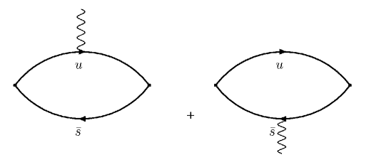
Figure 1: Quark flow diagrams for the $K^{*}$ meson.

We calculate each of the the quark sector contributions to the form factors separately, i.e. in Fig. 1 we calculate this amplitude with the photon striking the light- and heavy-quarks separately. The quark sector contributions are then combined to assemble observables. Following Brodsky and Hiller [3], for the pseudo-scalar mesons,

$$\left\langle p^{\prime}|J^{\alpha}|p\right\rangle=\frac{1}{2\sqrt{E_{p}E_{p^{\prime}}}}\,[p^{\alpha}+{p^{\prime}}^{\alpha}]F_{1}(Q^{2})$$

and for the vector mesons,

$$\left\langle p^{\prime},s^{\prime}|J^{\mu}|p,s\right\rangle = \ \frac{1}{2\sqrt{E_{p}E_{p^{\prime}}}}\,\epsilon^{\prime\star}_{\alpha}(p^{\prime},s^{\prime})\epsilon_{\beta}(p,s)J^{\alpha\mu\beta}(p^{\prime},p)$$

$$J^{\alpha\mu\beta}(p^{\prime},p) = -\bigg{\{}G_{1}(Q^{2})\,g^{\alpha\beta}\,[p^{\mu}+p^{\prime\mu}]+\ G_{2}(Q^{2})\,[g^{\mu\beta}q^{\alpha}-g^{\mu\alpha}q^{\beta}]+\ G_{3}(Q^{2})\,q^{\beta}q^{\alpha}\ \frac{p^{\mu}+p^{\prime\mu}}{2M^{2}}\bigg{\}}\ .$$

In our calculation the mesons initially have zero momentum and, after scattering with the photon, one unit of momentum in the final state. The final momentum is in the $x$-direction. The covariant vertex functions $G_{1}(Q^{2}),G_{2}(Q^{2})$, and $G_{3}(Q^{2})$ are related to the Sachs form factors [3] via,

$$G_{Q}(Q^{2}) = G_{1}(Q^{2})-G_{2}(Q^{2})+(1+\frac{Q^{2}}{4m^{2}})G_{3}(Q^{2})$$ (1)

$$G_{M}(Q^{2}) = G_{2}(Q^{2})$$ (2)

$$G_{C}(Q^{2}) = G_{1}(Q^{2})+\frac{2}{3}\frac{Q^{2}}{4m^{2}}G_{Q}(Q^{2})\,.$$ (3)

In this simulation $Q^{2}\simeq 0.22\ {\rm GeV}^{2}$.

On the lattice we define the three point function,

$$G^{\mu\alpha\nu}(t_{2},t_{1},\vec{p}\,^{\prime},\vec{p}) = \sum_{\vec{x_{1}},\vec{x_{2}}}e^{-i\vec{p^{\prime}}.(\vec{x_{2}}-\vec{x_{1}})}e^{-i\vec{p}.\vec{x_{1}}}\langle\Omega|\chi^{\mu}(x_{2})J^{\alpha}(x_{1})\chi^{\dagger\nu}(0)|\Omega\rangle$$

$$=\sum_{i,j}\sum_{s,s^{\prime}}e^{-E_{i}(t_{2}-t_{1})}e^{-E_{j}t_{1}}\ \langle\Omega|\chi^{\mu}|p^{\prime},s^{\prime}\rangle\langle p^{\prime},s^{\prime}|J^{\alpha}|p,s\rangle\langle p,s|\chi^{\dagger\nu}|\Omega\rangle\ ,$$

where the interpolator creates a meson at the source, the current is inserted at an intermediate time (time slice $t_{1}=14$), and finally the state is annihilated at the sink at $t_{2}$. We can show that the Sachs form factors can be extracted from linear combinations of the ratios,

$$R^{\mu\alpha\nu}(p^{\prime},p)=\sqrt{\frac{\left<G^{\mu\alpha\nu}(\vec{p^{\prime}},\vec{p},t,t_{1})\right>\,\left<G^{\nu\alpha\mu}(\vec{p},\vec{p^{\prime}},t,t_{1})\right>}{\bigg{<}G^{\mu\mu}(\vec{p^{\prime}},t)\bigg{>}\,\bigg{<}G^{\nu\nu}(\vec{p},t)\bigg{>}}}\ .$$

In this notation $\mu$ is the Lorentz index of the interpolator at the sink, $\alpha$ is the Lorentz index on the current insertion and $\nu$ is the Lorentz index of the interpolator source. It can be shown that,

$$G_{C}(Q^{2}) = \frac{2}{3}\frac{\sqrt{Em}}{E+m}\left(R^{101}+R^{202}+R^{303}\right)$$

$$G_{M}(Q^{2}) = \frac{\sqrt{Em}}{p_{x}}\left(R^{133}+R^{331}\right)$$

$$G_{Q}(Q^{2}) = \frac{m\sqrt{Em}}{p^{2}_{x}}\left(2R^{101}-R^{202}-R^{303}\right)\ .$$

The charge radius is defined in terms of the charge form factor as,

$$\langle r^{2}\rangle=-6\frac{\partial}{\partial Q^{2}}G(Q^{2}){\Big{|}}_{Q^{2}=0}\ .$$

Our lattice calculations are necessarily defined at finite $Q^{2}$, but we continue to $Q^{2}=0$ by assuming $G_{C}$ has a monopole form,

$$G_{C}(Q^{2})=\left(\frac{1}{\frac{Q^{2}}{\Lambda^{2}}+1}\right)\ ,$$

enabling the derivative to be taken. The lattice form factor calculation then defines $\Lambda$. Motivated by the scaling of $G_{M}(Q^{2})\over G_{C}(Q^{2})$ for baryons at small $Q^{2}$, we extrapolate $G_{M}(Q^{2})$ to $Q^{2}=0$ by assuming,

$$G_{M}(0)\simeq\frac{G_{M}(Q^{2})}{G_{C}(Q^{2})}\ ,$$

for individual quark sectors. In terms of the magnitude of the electron charge $e$ and the mass of the meson $M$, the magnetic moment is,

$$\mu_{1}=G_{M}(0){e\over 2M}\ .$$

Our simulations are done on a large $20^{3}\times 40$ lattice, $a=0.128$ fm with 380 gauge field configurations. Our definition of the conserved current is $O(a)$ improved and conserved [4, 5]. We use the FLIC fermion action. For further details of the simulation parameters used in this calculation see Zanotti et al. [6]. We note that the vector mesons are bound at all quark masses used in this calculation.

2 Results

We begin the discussion of our results with the charge radii of the vector and pseudo-scalar mesons. From the quark model we would expect a hyperfine interaction between the quark and anti-quark of the form $\frac{\vec{\sigma_{q}}\cdot\vec{\sigma_{\bar{q}}}}{m_{q}m_{\bar{q}}}$. The interaction is repulsive where the spins are aligned, as in the vector mesons, and attractive where the spins are anti-aligned, as in the pseudo-scalar mesons. In Fig. 2 we show the charge radii of the vector and pseudo-scalar mesons.

Figure 2: Summary of the meson and proton charge radii.

Indeed we find that the charge radii of the vector mesons are consistently larger than the pseudo-scalar mesons, and in fact similar to the charge radii of the proton.

Next in Fig. 3 we show the ratio of the light-quark contribution to the charge radii of the strange and non-strange mesons. We find that there is no evidence of the environmental sensitivity in the light-quark contribution the pseudo-scalar mesons. However we do find clear evidence of environmental sensitivity of the light-quark contribution to the vector mesons at our smaller quark masses. The broadening of the charge distribution in the $\rho^{+}$ is consistent with the hyperfine repulsion discussed above.

Figure 3: (Left) Ratio of the light-quark contribution to $<r^{2}>\ {\rm fm}^{2}$ in the pion and kaon. (Right) Ratio of the light-quark contribution to $<r^{2}>\ {\rm fm}^{2}$ in the $\rho^{+}$ and $K^{*+}$.

Next we present our analysis of the magnetic moments of the vector mesons. At the SU(3) flavour limit, the simple quark model predicts that the magnetic moment of the $\rho$ meson in nuclear magnetons is $\mu_{\rho}\simeq 1.84\mu_{N}$, three times the magnetic moment of the $\Lambda$ baryon. Our results are consistent with this prediction.

To easily compare with previous lattice simulations [7], in Fig. 4 we report the g-factor of the vector mesons. We note that our calculation is consistent with the previous lattice calculation.

Figure 4: (Left) G-factor of the $\rho$ meson. (Right) G-factor of the $K^{*}$ meson.

Finally in Fig. 5 we show the quadrupole form factor of the $\rho$. We find that the quadrupole form factor is less than zero indicating that the spatial distribution of charge within the $\rho$ meson is oblate. This is in accord with the findings of Alexandrou et al.[1].

Figure 5: $\rho$-meson quadrupole form factor at $Q^{2}\simeq 0.22\ {\rm GeV}^{2}$.

3 Conclusions

In conclusion, we find that the charge radii of the vector mesons are larger than the charge radii of the pseudoscalar mesons. Indeed we find that the trend in the charge radius of the vector mesons is similar to the charge radius of the proton. By evaluating the quark sector contributions to each observable separately we are able to determine that there is significant environmental sensitivity in the light-quark contributions to charge radii of the vector mesons. We find that the magnetic moment of the $\rho$ is consistent with quark model predictions at the SU(3) flavour limit, and with previous lattice simulations. Finally we determine that the quadrupole form factor of the $\rho$ meson is negative which means that the distribution of charge in the vector mesons is oblate.

References

• [1] C. Alexandrou, P. de Forcrand and A. Tsapalis, Probing hadron wave functions in lattice QCD, Phys. Rev. D66 (2002) 094503 [hep-lat/0206026].
• [2] J. N. Hedditch et. al., $1^{-+}$ exotic meson at light quark masses, Phys. Rev. D72 (2005) 114507 [hep-lat/0509106].
• [3] S. J. Brodsky and J. R. Hiller, Universal properties of the electromagnetic interactions of spin one systems, Phys. Rev. D46 (1992) 2141–2149.
• [4] G. Martinelli, C. T. Sachrajda and A. Vladikas, A study of ’improvement’ in lattice QCD, Nucl. Phys. B358 (1991) 212–230.
• [5] D. B. Leinweber, R. M. Woloshyn and T. Draper, Electromagnetic structure of octet baryons, Phys. Rev. D43 (1991) 1659–1678.
• [6] J. M. Zanotti, B. Lasscock, D. B. Leinweber and A. G. Williams, Scaling of FLIC fermions, Phys. Rev. D71 (2005) 034510 [hep-lat/0405015].
• [7] W. Andersen and W. Wilcox, Lattice charge overlap. i. elastic limit of pi and rho mesons, Annals Phys. 255 (1997) 34–59 [hep-lat/9502015].