UTHEP-537 First Nonperturbative Test of a Relativistic Heavy Quark Action
in Quenched Lattice QCD

Abstract

We perform a numerical test of a relativistic heavy quark(RHQ) action, recently proposed by Tsukuba group, in quenched lattice QCD at $a\simeq 0.1$ fm. With the use of the improvement parameters previously determined at one-loop level for the RHQ action, we investigate a restoration of rotational symmetry for heavy-heavy and heavy-light meson systems around the charm quark mass. We focused on two quantities, the meson dispersion relation and the pseudo-scalar meson decay constants. It is shown that the RHQ action significantly reduces the discretization errors due to the charm quark mass. We also calculate the S-state hyperfine splittings for the charmonium and charmed-strange mesons and the $D_{s}$ meson decay constant. The remaining discretization errors in the physical quantities are discussed.

I Introduction

For a search of new physics beyond the standard model through flavor physics, a precise determination of physical quantities such as quark masses and hadronic matrix elements associated with heavy mesons is required within a few % accuracy. Although, in principle, lattice QCD calculation is an ideal tool for this purpose, it suffers from large discretization effects due to the charm and bottom quark masses: $am_{c}\hbox to0.0pt{\lower 3.5pt\hbox{$\mathchar 0\relax\sim$}\hss}\raise 1.0pt\hbox{$>$}0.3$, $am_{b}\hbox to0.0pt{\lower 3.5pt\hbox{$\mathchar 0\relax\sim$}\hss}\raise 1.0pt\hbox{$>$}1$ in quenched approximation and $am_{c}\hbox to0.0pt{\lower 3.5pt\hbox{$\mathchar 0\relax\sim$}\hss}\raise 1.0pt\hbox{$>$}0.5$, $am_{b}\hbox to0.0pt{\lower 3.5pt\hbox{$\mathchar 0\relax\sim$}\hss}\raise 1.0pt\hbox{$>$}1.5$ in unquenched simulation with current computational resources. If we adopt the $O(a)$ improved Wilson quark action for the heavy quarks, the leading cutoff errors are expected to be $O((am_{Q})^{n})$. In order to achieve a few $\%$ accuracy, it is necessary to reduce the discretization errors for the heavy quarks to the same level for the light quarks, which is $O((a\Lambda_{\rm QCD})^{2})$.

For this end an on-shell $O(a{\Lambda}_{\rm QCD})$ improved RHQ action has been proposed in Ref.akt , which extends the well known on-shell improvement programsym1 ; sym2 ; sw ; alpha ; onshell to massive quarks with $am_{Q}\sim O(1)$. The action works better as the lattice spacing becomes smaller. This is a fascinating feature from a view point of controlling the systematic errors coming from the cutoff effects. Another important point is that the action allows to treat the charm and bottom quarks simultaneously. In case of NRQCD, widely used for calculation of the bottom quark physics, on the other hand, it is theoretically impossible to take the continuum limit and difficult to treat the charm quark.

The explicit form of the RHQ action is given by

$$S^{\rm RHQ} = \sum_{x}\left[m_{0}{\bar{q}}(x)q(x)+{\bar{q}}(x)\gamma_{4}D_{4}q(x)+\nu\sum_{i}{\bar{q}}(x)\gamma_{i}D_{i}q(x)\right.$$

$$\left.-\frac{r_{t}a}{2}{\bar{q}}(x)D_{4}^{2}q(x)-\frac{r_{s}a}{2}\sum_{i}{\bar{q}}(x)D_{i}^{2}q(x)\right.$$

$$\left.-\frac{iga}{2}{\it c}_{\it E}\sum_{i}{\bar{q}}(x)\sigma_{4i}F_{4i}q(x)-\frac{iga}{4}{\it c}_{\it B}\sum_{i,j}{\bar{q}}(x)\sigma_{ij}F_{ij}q(x)\right],$$

where four improvement parameters $\nu$, $r_{s}$, $c_{E}$ and $c_{B}$ are relevant, while $r_{t}$ is redundant. The leading cutoff effects of $O((am_{Q})^{n})$ in this formulation can be removed by adjusting $\nu$ and quark field renormalization factor as a function of $am_{Q}$ and gauge coupling constant $g$. We can also remove the next-to-leading cutoff effects of $O((am_{Q})^{n}a{\Lambda}_{\rm QCD})$ by adjusting $r_{s}$, $c_{E}$ and $c_{B}$. Note that it is recently pointed out that one can remove $O((am_{Q})^{n}a{\Lambda}_{\rm QCD})$ errors in the spectral quantities such as masses by adjusting only two parameters, $c_{B}=c_{E}$ and $\nu$Christ . However it is still true that 4 parameters, $\nu$, $r_{s}$, $c_{E}$ and $c_{B}$, are necessary to remove all $O((am_{Q})^{n}a{\Lambda}_{\rm QCD})$ errors in on-shell matrix elements. Once these are achieved, we are left with only the cutoff effects of $O(f_{2}(am_{Q})(a{\Lambda}_{\rm QCD})^{2})$ where $f_{2}(am_{Q})$ is an analytic function of $am_{Q}$ around $am_{Q}=0$. We assume $f_{2}(am_{Q})\sim O(1)$ for the massive quarks with $m_{Q}a\sim O(1)$. In the massless limit $\nu$ and $r_{s}$ become unity and $c_{E}$ and $c_{B}$ agree with $c_{\rm SW}$. Since, at present, it is difficult to determine $r_{s}$, $c_{E}$, $c_{B}$ nonperturbatively, we have performed a perturbative determination of the four parameters at one-loop level in a mass dependent waycEcB . In this case the remaining leading cutoff effects are $O(\alpha_{s}^{2}f_{0}^{(2)}(am_{Q}))$ for the RHQ action. Similarly, we have also determined the mass-dependent renormalization constants and the improvement coefficients for the vector and axial-vector currents at one-loop levelzAcA .

In this work we study the discretization effects of the RHQ action with the perturbatively determined improvement parameters using two different gauge actions in quenched approximation at a finite lattice spacing of $a\simeq 0.1$fm. We employ four heavy quark masses around the charm quark mass. In order to investigate the discretization effects, we calculate the dispersion relation both for the heavy-heavy and heavy-light mesons and the space-time symmetry of the pseudo-scalar meson decay matrix elements. For comparison, the same calculation is repeated with the heavy clover quark action. We observe sufficient reduction of $(am_{Q})^{n}$ errors in the RHQ action. In addition we extract the charmed-strange and charmonium hyperfine splittings and the $D_{s}$ meson decay constant $f_{D_{s}}$ at the physical charm quark mass. We compare our results with previous ones and discuss the cutoff effects on these quantities with the RHQ quark action.

This paper is organized as follows. In Sect. II we explain the RHQ action and fix the notations. Simulation details are summarized in Sect. III. In Sect. IV we give a comparison between the RHQ action and the clover action by showing the dispersion relation and the space-time symmetry. We also present the results of physical quantities such as the hyperfine splittings and the decay constants, and discuss their cutoff errors in detail. A comparison of our results with the previous ones for the hyperfine splittings and the decay constants is also shown. In Sect. V we give our conclusion. A brief review of recent works related to this formulation can be found in Ref.KrmshNote .

II FORMULATION

II.1 Actions

For the gauge part we employ a renormalization-group (RG) improved gauge action proposed by Iwasakiiwasaki as well as the ordinary plaquette gauge action. For the quark part we use the clover quark actionsw for the light quarks and the RHQ action for the heavy quarks. We rewrite the RHQ action of Eq.(I) to the following form with the use of hopping parameter $\kappa$, which is more suitable for numerical simulations:

$$S^{\rm RHQ} = \sum_{x,y}\overline{q}(x)D_{x,y}q(y),$$ (2)

$$D_{x,y} = \delta_{xy}-\kappa\sum_{k=1,3}\left\{(r_{s}-\nu\gamma_{k})U_{x,k}\delta_{x+\hat{k},y}+(r_{s}+\nu\gamma_{k})U_{x,k}^{{\dagger}}\delta_{x,y+\hat{k}}\right\}$$ (3)

$$-\kappa\left\{(r_{t}-\gamma_{4})U_{x,4}\delta_{x+\hat{4},y}+(r_{t}+\gamma_{4})U_{x,4}^{{\dagger}}\delta_{x,y+\hat{4}}\right\}$$

$$-\,\delta_{xy}c_{B}\kappa\sum_{i<j}\sigma_{ij}F_{ij}(x)-\,\delta_{xy}c_{E}\kappa\sum_{i}\sigma_{4i}F_{4i}(x),$$

where the field strength $F_{\mu\nu}$ in the clover terms is expressed as

$$F_{\mu\nu}(x) = \frac{1}{8}\sum_{i=1}^{4}\left(U_{i}(x)-U_{i}^{\dagger}(x)\right),$$ (4)

$$U_{1}(x) = U_{x,\mu}U_{x+{\hat{\mu}},\nu}U^{\dagger}_{x+{\hat{\nu}},\mu}U^{\dagger}_{x,\nu},$$ (5)

$$U_{2}(x) = U_{x,\nu}U^{\dagger}_{x-{\hat{\mu}}+{\hat{\nu}},\mu}U^{\dagger}_{x-{\hat{\mu}},\nu}U_{x-{\hat{\mu}},\mu},$$ (6)

$$U_{3}(x) = U^{\dagger}_{x-{\hat{\mu}},\mu}U^{\dagger}_{x-{\hat{\mu}}-{\hat{\nu}},\nu}U_{x-{\hat{\mu}}-{\hat{\nu}},\mu}U_{x-{\hat{\nu}},\nu},$$ (7)

$$U_{4}(x) = U^{\dagger}_{x-{\hat{\nu}},\nu}U_{x-{\hat{\nu}},\mu}U_{x+{\hat{\mu}}-{\hat{\nu}},\nu}U^{\dagger}_{x,\mu}.$$ (8)

As mentioned in the introduction, the parameters $\nu$, $r_{s}$, $c_{B}$ and $c_{E}$ are already determined as a function of the heavy quark mass up to one-loop level. In this work we choose $r_{t}=1$.

II.2 Improvement of axial vector current

The form of renormalized axial vector current with the $O(a{\Lambda}_{\rm QCD})$ improvement is given in Ref.zAcA :

$$A^{R}_{\mu}(x) = \sqrt{2\kappa_{q}}\sqrt{2\kappa_{Q}}Z_{A_{\mu}}\left[~{}{\bar{q}(x)}\gamma_{\mu}\gamma_{5}Q(x)-c_{A_{\mu}}^{+}\{{\bar{q}(x)}\Delta_{\mu}^{+}\gamma_{5}Q(x)\}-c_{A_{\mu}}^{-}\{{\bar{q}(x)}\Delta_{\mu}^{-}\gamma_{5}Q(x)\}\right.$$ (9)

$$\left.+c_{A_{\mu}}^{L}\{{\vec{\Delta}_{i}}{\bar{q}(x)}\}\gamma_{i}\gamma_{\mu}\gamma_{5}Q(x)-c_{A_{\mu}}^{R}{\bar{q}(x)}\gamma_{\mu}\gamma_{5}\gamma_{i}\{{\vec{\Delta}_{i}}Q(x)\}~{}\right],$$

where $q$ and $Q$ denote the light and heavy quark fields, respectively. $Z_{A_{\mu}}$ is the finite renormalization factor connecting the lattice to the continuum ${\overline{\rm MS}}$ scheme ($Z_{A}=Z_{A_{\mu}}^{\rm latt}/Z_{A_{\mu}}^{\rm cont}$) as defined in Ref.zAcA . Improvement coefficients for the temporal direction are in general different from those for the spatial direction: $c_{A_{4}}^{\pm,R,L}\not=c_{A_{k}}^{\pm,R,L}$. An additional overall factor $\sqrt{2\kappa_{q}}\sqrt{2\kappa_{Q}}$ is associated with the field redefinition in the RHQ action of Eq.(3). $Z_{A_{\mu}}$ and $c_{A_{\mu}}^{\{\pm,R,L\}}$ are calculated as a function of the quark masses $am_{Q}$ and $am_{q}$ up to one-loop levelzAcA . With the aid of the equation of motion we can always choose $c^{R}_{A_{4}}=c^{L}_{A_{4}}=0$. Covariant lattice derivatives $\Delta_{\mu}^{+}$ and $\Delta_{\mu}^{-}$ are defined as $\Delta_{\mu}^{+}=\Delta\raisebox{7.74998pt}{$\rightarrow$}_{\mu}+\Delta\raisebox{7.74998pt}{$\leftarrow$}_{\mu}$ and $\Delta_{\mu}^{-}=\Delta\raisebox{7.74998pt}{$\rightarrow$}_{\mu}-\Delta\raisebox{7.74998pt}{$\leftarrow$}_{\mu}$, where $\Delta\raisebox{7.74998pt}{$\rightarrow$}_{\mu}$ and $\Delta\raisebox{7.74998pt}{$\leftarrow$}_{\mu}$ are lattice derivative acting on the right or left field as

$${\bar{q}(x)}~{}\gamma_{5}~{}\Delta\raisebox{7.74998pt}{$\rightarrow$}_{\mu}~{}Q(x) = {\bar{q}(x)}~{}\gamma_{5}~{}\frac{1}{2}[~{}U_{\mu}(x)Q(x+{\hat{\mu}})-U_{\mu}^{\dagger}(x-{\hat{\mu}})Q(x-{\hat{\mu}})~{}],$$ (10)

$${\bar{q}(x)}~{}\Delta\raisebox{7.74998pt}{$\leftarrow$}_{\mu}~{}\gamma_{5}~{}Q(x) = \frac{1}{2}[~{}{\bar{q}(x+{\hat{\mu}})}U_{\mu}^{\dagger}(x)-{\bar{q}(x-{\hat{\mu}})}U_{\mu}(x-{\hat{\mu}})~{}]~{}\gamma_{5}~{}Q(x).$$ (11)

Note that the definition of the improved current of Eq.(9) is slightly modified from that in Ref.zAcA . The difference will be explained in Appendix A. Hereafter we use a short-handed notation for the improvement terms such as

$$O_{\mu}^{+} \equiv -c_{A_{\mu}}^{+}\{{\bar{q}(x)}\Delta_{\mu}^{+}\gamma_{5}Q(x)\},$$ (12)

$$O_{\mu}^{-} \equiv -c_{A_{\mu}}^{-}\{{\bar{q}(x)}\Delta_{\mu}^{-}\gamma_{5}Q(x)\},$$ (13)

$$O_{k}^{L} \equiv +c_{A_{k}}^{L}\{{\Delta\raisebox{7.74998pt}{$\rightarrow$}_{i}}{\bar{q}(x)}\}\gamma_{i}\gamma_{k}\gamma_{5}Q(x),$$ (14)

$$O_{k}^{R} \equiv -c_{A_{k}}^{R}{\bar{q}(x)}\gamma_{k}\gamma_{5}\gamma_{i}\{{\Delta\raisebox{7.74998pt}{$\rightarrow$}_{i}}Q(x)\}.$$ (15)

The pseudo-scalar meson decay constant is defined as

$$\left<0|A_{\mu}^{R}(0)|PS(p)\right> = ip_{\mu}f_{PS}(A_{\mu}),$$ (16)

where $|PS(p)\rangle$ is the pseudo-scalar meson state with momentum $p$. The decay constant denoted as $f_{PS}(A_{\mu})$ identifies which component of the axial vector current is used. In the continuum limit $f_{PS}(A_{\mu})$ for different $\mu$ should agree with each other.

III simulation details

III.1 Simulation parameters

We employ a single value of the gauge coupling constant, $\beta=2.6$ for the Iwasaki action and $\beta=6.0$ for the plaquette action, on a $L^{3}\times T=24^{3}\times 48$ lattice. Gauge configurations are generated by a 5-hit pseudo heat bath update supplemented by four over-relaxation steps. These configurations are then fixed to the Coulomb gauge at every 100 sweeps for the Iwasaki gauge action and 200 sweeps for the plaquette gauge action. We have accumulated $300$ gauge configurations for each gauge action with the RHQ action and 250 with the heavy clover quark action. With the use of the Sommer scale $r_{0}=0.5$fm the lattice cutoffs are determined as $a^{-1}(r_{0})=2.0129(46)[{\rm GeV}]$ r0Necco and $a^{-1}(r_{0})=2.1184(94)[{\rm GeV}]$ r0Sommer , respectively. The spatial lattice size in physical unit is approximately $2.4$fm, which is large enough for the charmed mesons.

Simulation parameters for the quark part are summarized in Table 1 for the Iwasaki and the plaquette gauge actions, where $M_{PS}/M_{V}$ represents the pseudo-scalar to vector meson mass ratio of the light-light and heavy-heavy mesons. For each gauge action we adopt three values of the light quark masses corresponding to $M_{PS}/M_{V}\simeq 0.55-0.78$ to cover the strange quark mass and four values of the heavy quark masses to sandwich the charm quark mass.

For the light quarks we use the clover quark action with the nonperturbative value of the clover coefficient: $c_{\rm SW}^{\rm NP}=1.50(5)$NPCL.CPPACS for the Iwasaki action and $1.769$NPCL.ALPHA for the plaquette action. Here it is noted that $c_{\rm SW}^{\rm NP}=1.50(5)$ for the Iwasaki action is taken from the preliminary result obtained in the infinite volume limit, which is 6 % larger than the final value $c_{\rm SW}^{\rm NP}=1.41$ of Ref.NPCL.CPPACS defined on a fixed physical volume. For the heavy quarks we adopt the RHQ action with the improvement parameters $\nu$, $r_{s}$, $c_{E}$ and $c_{B}$ determined up to one-loop level with the mean-field(MF) improvement, details of which are explained in Appendix A. In order to remove $O(a{\Lambda}_{\rm QCD})$ errors at the massless point, we replace a massless part of $c_{E}$ and $c_{B}$ by their nonperturbative value $c_{\rm SW}^{\rm NP}$ as

$$c_{E,B}=c_{E,B}^{\rm PT}(am_{\rm pole})-c_{E,B}^{\rm PT}(am_{\rm pole}=0)+c_{\rm SW}^{\rm NP},$$ (17)

where the superscript PT represents the perturbative value up to one-loop level.

For the light-light current we use nonperturbative values of the renormalization factor and the improvement coefficients for the plaquette gauge action: $Z_{A}^{\rm NP}=0.807$, $b_{A}^{\rm NP}=1.28$ and $c_{A}^{\rm NP}=0.037$NPzAcA:LALM:3 . For the Iwasaki gauge action we employ the mean-field improved values: $Z_{A}=0.86057$, $b_{A}=1.19998$ and $c_{A}=0.00864$gmass . At present nonperturbative values are not available for this action. For the heavy-light and heavy-heavy currents, on the other hand, we use the mean-field improved values for $c_{A_{\mu}}^{\{\pm,L,R\}}$ and $Z_{A_{\mu}}$ at the one-loop level (see Appendix A) for both gauge actions. In case of the plaquette gauge action we replace the massless part of $c_{A_{\mu}}^{+}$ and $Z_{A_{\mu}}$ by the nonperturbative ones, $c_{A}^{\rm NP}$ and $Z_{A}^{\rm NP}$:

$$c_{A_{\mu}}^{+} = g^{2}c_{A_{\mu}}^{+,{\rm PT}}(am_{\rm pole})-g^{2}c_{A_{\mu}}^{+,{\rm PT}}(am_{\rm pole}=0)+c_{A}^{+,{\rm NP}},$$ (18)

$$Z_{A_{\mu}} = Z_{A_{\mu}}^{\rm PT}(am_{\rm pole})-Z_{A_{\mu}}^{\rm PT}(am_{\rm pole}=0)+Z_{A_{\mu}}^{\rm NP}.$$ (19)

In order to investigate a degree of improvement for the RHQ action we have made an additional simulation using the clover quark action both for the heavy and light quarks. Simulation parameters are given in Table 2, where we employ one value of the light quark mass and three values of the heavy quark masses roughly equal to lighter three for the RHQ action.

On each configuration fixed with the Coulomb gauge, we invert the quark matrix employing the BiCGstab algorithm with the stopping condition that the residual must be smaller than $1.0\times 10^{-14}$. For the heavy quarks we perform a fixed number of iterations. We choose $2T=96$ such that the stopping condition is always satisfied and it is assured that the heavy quarks can propagate from the origin to any point on the lattice. For both the light and heavy quark propagators we employ not only a local source but also an exponentially smeared source with a form of $A\exp(-Br)$, where smearing parameters $A$ and $B$ are tuned to enhance an overlap with the ground state. Numerical values of $A$ and $B$ are listed in Table 3 for each combination of the gauge and quark actions.

III.2 Measurement of two-point functions

We measure the S-state (i.e. pseudo-scalar and vector) meson spectra for the light-light(L-L), heavy-light(H-L) and heavy-heavy(H-H) systems using the correlation functions projected onto zero spatial momentum state:

$$\sum_{\vec{x}}\langle{\cal O}_{L}(\vec{x},t){\cal O}_{S,L}^{\dagger}(0)\rangle,$$ (20)

where ${\cal O}=P$ or $V$ is understood. The subscripts $S$ and $L$ represent the smeared and local operators, respectively. We always adopt a local sink while taking both the local and smeared sources. Note that both the quark and anti-quark fields in ${\cal O}_{S}$ are smeared.

To extract the pseudo-scalar meson decay constant for the L-L, H-L, H-H systems, we calculate the correlation function

$$\sum_{\vec{x}}\langle A_{4}^{\rm impr}(\vec{x},t)P_{S}^{\dagger}(0)\rangle,$$ (21)

where the superscript impr represents the $O(a)$ improved current given in Eq.(9).

We also measure the meson correlation functions with finite spatial momenta given by

$$a{\vec{p}}=\frac{2\pi}{L}\times\{(1,0,0),\ (1,1,0)\}.$$ (22)

These correlation functions are used to calculate the dispersion relation of the S-state mesons and also to extract the decay constant using the temporal and spatial components of the axial vector current.

III.3 Fitting procedure

The correlation functions in Eq.(20) are expected to take the following form for a large euclidean time separation:

$$\Sigma_{\vec{x}}\langle{\cal O}_{L}(\vec{x},t){\cal O}_{S,L}^{\dagger}(0)\rangle=\frac{Z_{{\cal O}_{L}}Z^{\dagger}_{{\cal O}_{S,L}}}{2aM}{\rm e}^{-aMT/2}\cosh(aM(T/2-t)),$$ (23)

$$\Sigma_{\vec{x}}\langle A^{\rm impr}_{\mu}(\vec{x},t)P_{S}^{\dagger}(0)\rangle=\frac{Z_{A^{\rm impr}_{\mu}}Z^{\dagger}_{P_{S}}}{2aM}{\rm e}^{-aMT/2}\sinh(aM(T/2-t)),$$ (24)

where $M$ is a mass of the ground state allowed to couple to the operator. Matrix elements in the above expressions are given by

$$Z_{P_{S,L}} = \langle 0|P_{S,L}(0)|PS(\vec{p}=\vec{0})\rangle,$$ (25)

$$Z_{V_{S,L}} = \langle 0|V_{S,L}(0)|V(\vec{p}=\vec{0})\rangle,$$ (26)

$$Z_{A^{\rm impr}_{\mu}} = \langle 0|A_{\mu}^{\rm impr}(0)|PS(\vec{p}=\vec{0})\rangle,$$ (27)

where $|PS(\vec{p}=\vec{0})\rangle$ and $|V(\vec{p}=\vec{0})\rangle$ represent the pseudo-scalar and vector meson states at rest. We first extract $aM$ by fitting the correlators of Eq.(23), and then perform a fit of Eq.(24) with $aM$ fixed. We employ the same fitting procedure for the correlation functions with finite spatial momenta. Since our statistics are not sufficient to incorporate correlations between different time slices, we always use the uncorrelated fit for our analysis. We estimate statistical errors by the jackknife method with a bin size of 10 configurations to eliminate autocorrelations. In case that the correlated fit is possible, we use it to check the results obtained by the uncorrelated fit. We find that the results are consistent within statistical errors.

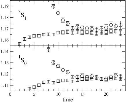
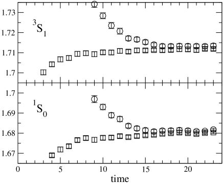
Figure 1: Effective mass plots for the H-L(left) and H-H(right) mesons with zero spatial momentum in case of $\kappa_{heavy}=\kappa_{6}$ and $\kappa_{light}=\kappa_{3}$ with the Iwasaki gauge action. Circles represent the local source correlators and squares for the smeared source correlators.

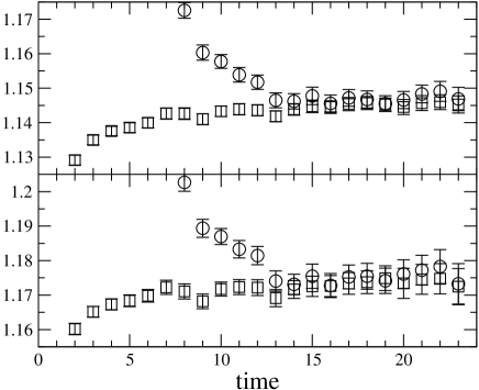
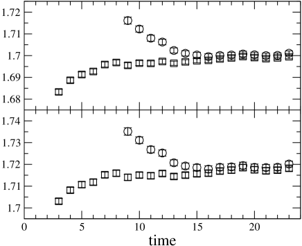
Figure 2: Effective mass plots for the H-L(left) and H-H(right) pseudoscalar mesons with $|a{\vec{p}}|^{2}=(2\pi/L)^{2}$ (top) and $|a{\vec{p}}|^{2}=2(2\pi/L)^{2}$ (bottom) in case of $\kappa_{heavy}=\kappa_{6}$ and $\kappa_{light}=\kappa_{3}$ with the Iwasaki gauge action. Circles represent the local source correlators and squares for the smeared source correlators.

The fitting ranges summarized in Table 4 are chosen by investigating effective mass plots of the meson correlators presented in Fig.1, where we take $\kappa_{3}$ for the light quark and $\kappa_{6}$ for the heavy quark as a representative case. Note that $\kappa_{6}$ roughly corresponds to the charm quark mass. We take similar fitting ranges for the correlators with finite spatial momenta, which are given in Table4. Figure 2 shows effective mass plots for the pseudo-scalar meson correlators with finite spatial momenta.

IV RESULTS

IV.1 Dispersion relation and space-time interchange symmetry

In case that the improvement parameters are perturbatively determined up to one-loop level, the leading cutoff errors in the RHQ action is theoretically expected to be $O(\alpha_{s}^{2}f_{0}^{(2)}(am_{Q}))$, where $f_{0}^{(2)}(am_{Q})\sim O(1)$ is assumed for $am_{Q}\sim O(1)$. We numerically check this theoretical expectation by investigating the dispersion relation of the S-state mesons and the space-time interchange symmetry for the pseudo-scalar meson decay constant. These quantities are sensitive to the cutoff effects for the heavy quarks, and hence suitable to estimate a size of $f_{0}^{(2)}(am_{Q})$.

We calculate an effective speed of light $c_{\rm eff}$ both for the pseudo-scalar and vector mesons by fitting the meson energy $aE({\vec{p}})$ as a function of the spatial momentum $a{\vec{p}}$ with the following form:

$$(aE({\vec{p}}))^{2}=c_{\rm eff}^{2}|a{\vec{p}}|^{2}+(aE({\vec{0}}))^{2}.$$ (28)

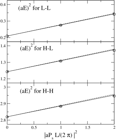
Figure 3: Momentum dependence of the pseudoscalar meson energies for the light-light system(top), the heavy-light system(middle) and the heavy-heavy(bottom) systems in case of $\kappa_{heavy}=\kappa_{6}$ and $\kappa_{light}=\kappa_{3}$ with the Iwasaki gauge action. The dashed line represents the continuum dispersion relation with $c_{\rm eff}=1$, while the solid one represents the fitting results with a linear function.

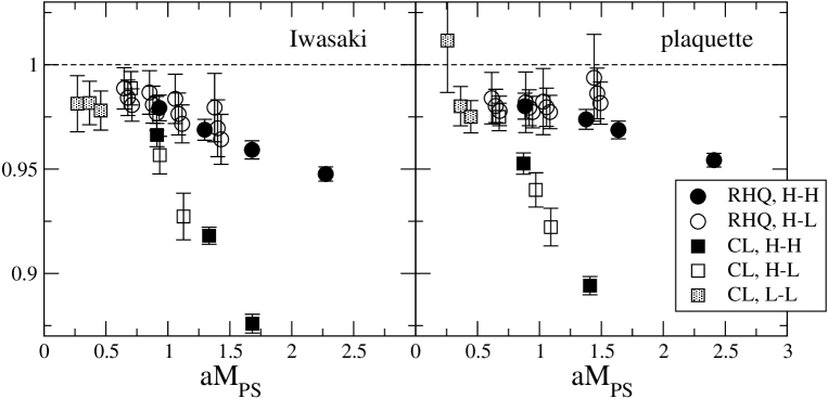
Figure 4: Effective speed of light for the heavy-heavy and heavy-light pseudoscalar mesons using the RHQ action and the heavy clover quark action with the Iwasaki(left) and the plaquette(right) gauge actions.

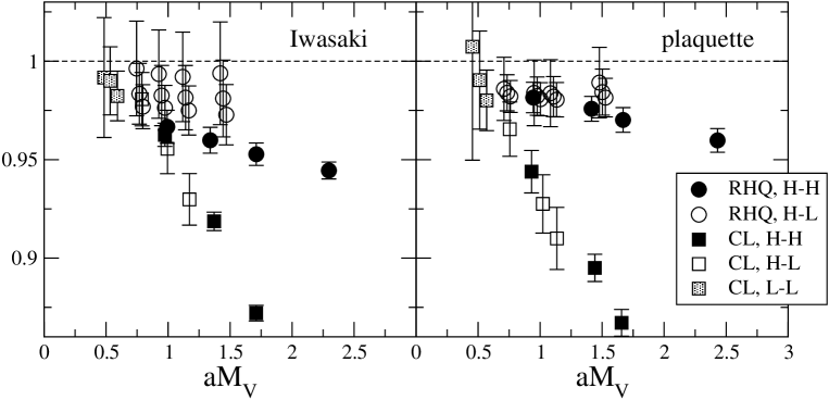
Figure 5: Same as Fig.4 for the vector mesons.

In the continuum limit $c_{\rm eff}$ should become unity. At finite lattice spacing, however, $c_{\rm eff}$ deviates from unity due to the lattice cutoff errors. In Fig.3 $(aE)^{2}$ is plotted as a function of $(a{\vec{p}})^{2}$, where the fitting result with Eq. (28) is given by the solid line together with the continuum dispersion relation with $c_{\rm eff}=1$ represented by the dashed line. We observe that the linearity of $E^{2}$ in $|{\vec{p}}|^{2}$ is well satisfied and $c_{\rm eff}$ is close to unity. Fitted values of $c_{\rm eff}$ for the L-L, H-L and H-H cases are plotted in Fig. 4 for the pseudo-scalar mesons and in Fig. 5 for the vector mesons. Here it should be noted that in addition to finite quark mass errors $c_{\rm eff}$ suffers from finite momentum corrections of $O(|a\vec{p}|^{2})$ so that $c_{\rm eff}$ could deviate from unity even for the massless quarks. Indeed Fig.4 shows that as the meson mass $Ma$ decreases, $c_{\rm eff}$ becomes closer to unity within this uncertainty. In the heavy quark mass region around $Ma\sim 1-2$, $c_{\rm eff}$ for the heavy clover quark action deviates from unity by about $7-10\%$. On the other hand, the RHQ action satisfies $c_{\rm eff}=1$ within $2-3\%$ errors, which are comparable to the deviation for the L-L case. Since fitted values of $c_{\rm eff}$ for the vector mesons in Fig. 5 are consistent with those for the pseudo-scalar mesons within statistical errors, we use the values of $c_{\rm eff}$ determined from the pseudo-scalar meson dispersion relation in the following discussion. We observe no obvious difference in the results between the Iwasaki and plaquette gauge actions.

We also study the space-time symmetry of the pseudo-scalar meson decay matrix element defined by

$$R\equiv i\frac{\langle 0|A_{k}^{R}|PS({\vec{p}})\rangle}{\langle 0|A_{4}^{R}|PS({\vec{p}})\rangle}\frac{E_{PS}}{|p_{k}|},$$ (29)

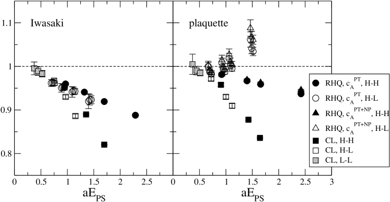
Figure 6: $R$ function defined by Eq.(29) for the heavy-heavy and heavy-light pseudoscalar mesons using the RHQ action and the heavy clover quark action with the Iwasaki(left) and the plaquette(right) gauge actions.

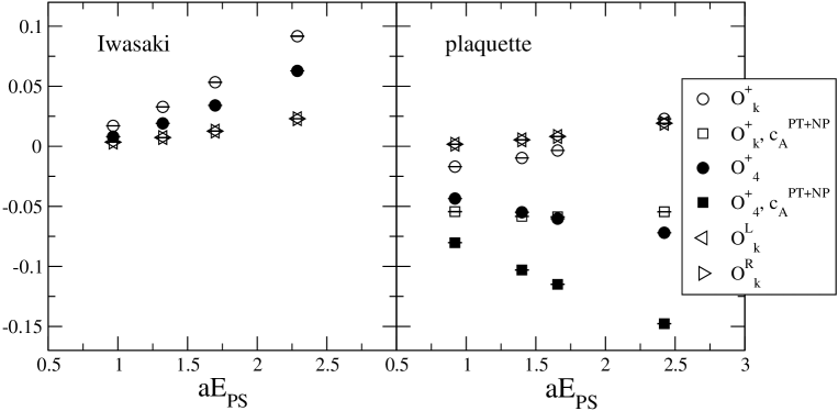
Figure 7: Contribution of each improvement term normalized by the diagonal one for the heavy-heavy axial vector current.

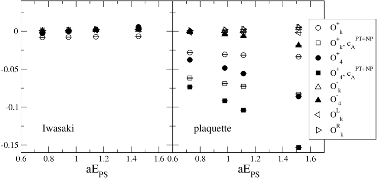
Figure 8: Same as Fig.7 for the heavy-light axial vector current.

where $A_{k}^{R}$ and $A_{4}^{R}$ represent the spatial and temporal components of the renormalized axial vector current given in Eq.(9). The pseudo-scalar meson state has finite spatial momentum of $|a\vec{p}|=2\pi/24$. The ratio $R$ is plotted in Fig.6 as a function of the meson energy $E_{PS}$ with the lowest finite spatial momentum for the L-L, H-L and H-H systems, where $c_{A}^{\rm PT+NP}$ represents the partial replacement of the perturbative value for $c_{A_{\mu}}^{+}$ by the nonperturbative one defined in Eq.(18), while $c_{A}^{\rm PT}$ means the perturbative value for $c_{A_{\mu}}^{+}$ without this replacement. For the plaquette gauge action we employ $Z_{A_{\mu}}$ defined in Eq.(19), though $Z_{A_{\mu}}^{\rm PT}=0.814$ and $Z_{A_{\mu}}^{\rm NP}=0.807$ agree with each other within $1\%$. Although because of the finite momentum corrections the ratio $R$ could deviate from unity even for the massless quarks, it becomes consistent with unity within the statistical errors as the meson energy $aE$ vanishes. For the massive mesons with $aE\sim 1-2$, on the other hand, the heavy clover quark action violates the space-time symmetry by about $7-13\%$, while the RHQ action retains $R=1$ within $6\%$ errors. An intriguing observation is that the ratio $R$ of the H-L system shows different $aE_{PS}$ dependences between the Iwasaki and plaquette gauge actions: the ratio $R$ decreases for the Iwasaki action as $E_{PS}$ increases, while it increases for the plaquette action. This different behaviors could come from a fact that the contributions of the $O(a)$ improvement operators are sizable for the plaquette action, whereas they are small for the Iwasaki action. This is observed in Figs.7 and 8 which show the relative contribution from each $O(a)$ improvement operator of Eqs.(12)-(15) to the axial-vector currents defined by

$$\frac{\sum_{\vec{x}}{\langle O_{\mu}^{\{\pm,L,R\}}({\vec{x}},t)P(0)\rangle}}{\sum_{\vec{x}}{\langle A_{\mu}({\vec{x}},t)P(0)\rangle}}.$$ (30)

Dominant contributions always come from $O_{\mu}^{+}$ operators for the plaquette action, while their contributions are not so large for the Iwasaki action. In particular, this feature is more prominent for the H-L system.

From the above analyses on $c_{\rm eff}$ and $R$ it can be concluded that the RHQ action succeeds in significantly reducing the $(m_{Q}a)^{n}$ errors in the heavy clover quark action.

IV.2 Physical quantities of S-state charmed mesons

IV.2.1 Physical points

In order to obtain the meson spectra and the decay constants at the physical quark masses, we have to interpolate the heavy quark mass to the charm quark mass $m_{c}$, while extrapolating the light quark mass to the $u,d$ quark mass $m_{ud}$ or interpolating it to the strange quark mass $m_{s}$. Since we employ only 3 values of the light quark masses in our simulation, we consider only a linear extrapolation to the $u,d$ quark mass. In the following the lattice spacing is always determined by the Sommer scale with $r_{0}=0.5$fm.

The light-light pseudo-scalar meson masses are linearly fitted in $1/\kappa$ as

$$a^{2}M_{PS}^{2}=A\left(\frac{1}{\kappa_{light}}-\frac{1}{\kappa_{crit}}\right),$$ (31)

where $\kappa_{crit}$ is determined from the vanishing point of $(aM_{PS})^{2}$. $\kappa_{ud}$ and $\kappa_{s}$ are determined so as to satisfy $M_{PS}=M_{\pi}=135.0$MeV and $M_{PS}=M_{K}=497.7$MeV, respectively. The fitting results of $A$ and $\kappa_{crit}$ are tabulated in Table 5 and $\kappa_{ud}$ and $\kappa_{s}$ are given in Table 6.

We determine $\kappa_{c}$ in two different ways: matching $M_{PS}^{\rm pole}$ to $M_{D_{s}}=1.9683$GeV for the charmed-strange meson or $M_{V}^{\rm pole}$ to $M_{J/\psi}=3.0969$GeV for the charmonium, where the superscript pole represents a pole mass determined from an exponential fall-off of the meson correlator. Employing the following fitting functions

$$aM_{PS}^{\rm pole}=A+B\kappa_{heavy}+C\kappa_{heavy}^{2}+Dam_{q}^{light}$$ (32)

for the heavy-light meson masses with $am_{q}^{light}=(1/\kappa_{light}-1/\kappa_{crit})/2$ and

$$aM_{V}^{\rm pole}=A+B\kappa_{heavy}+C\kappa_{heavy}^{2}$$ (33)

for the heavy-heavy meson masses, we have determined two values of $\kappa_{c}$, which are given in Table 6.

In order to estimate a magnitude of the cutoff errors, we also calculate the charmed meson spectra employing the kinetic mass defined by

$$aM^{\rm kin}=aM^{\rm pole}/c_{\rm eff}^{2}.$$ (34)

With the same fitting functions as Eqs.(32) and (33) we have also determined $\kappa_{c}(D_{s},M^{\rm kin})$ and $\kappa_{c}(J/\psi,M^{\rm kin})$ listed in Table 6. From these results we observe that a difference of $\kappa_{c}$ between two physical inputs $M_{J/\psi}$ and $M_{D_{s}}$ is less than $0.2\%$, while a difference of $\kappa_{c}$ between $M^{\rm pole}$ or $M^{\rm kin}$ is about $2\%$. In the following analysis, we always calculate all the physical quantities using both $M^{\rm pole}$ and $M^{\rm kin}$, in order to estimate the systematic errors due to an ambiguity in the choice of $M^{\rm pole}$ or $M^{\rm kin}$.

IV.2.2 Hyperfine splitting for charmonium and charmed-strange meson

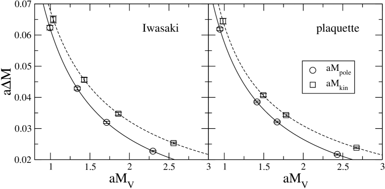
Figure 9: Heavy-heavy meson S-state hyperfine splittings as a function of $M_{V}a$.

Figure 9 shows $aM_{V}^{X}$ dependence of the S-state charmonium hyperfine splitting $a\Delta M^{X}=aM_{V}^{X}-aM_{PS}^{X}$, where $X=$ pole or kin. In order to interpolate the results at the physical charm quark mass, we adopt the ansatz that the splitting is a polynomial of the inverse vector meson mass:

$$a\Delta M^{X}=A/(aM_{V}^{X})+B/(aM_{V}^{X})^{2}+C/(aM_{V}^{X})^{3},$$ (35)

incorporating a property that the hyperfine splitting vanishes in the infinite quark mass limit due to the heavy quark symmetry. The interpolation lines are also plotted in Fig.9. Using the fitting results for the parameters $A$, $B$ and $C$ given in Table 7, we obtain $\Delta M(J/\psi-\eta_{c})$ in physical unit. $\Delta M^{\rm pole}$ at $\kappa_{c}(J/\psi,M^{\rm pole})$ and $\Delta M^{\rm kin}$ at $\kappa_{c}(J/\psi,M^{\rm kin})$ are tabulated in Table 8 for each gauge action together with the experimental value.

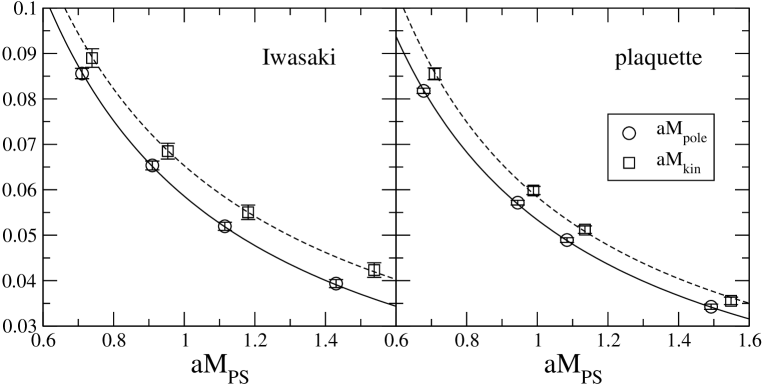
Figure 10: Heavy-light meson S-state hyperfine splittings as a function of $aM_{PS}$ with $\kappa_{light}=\kappa_{3}$.

In Fig.10 we plot the S-state charmed-strange meson hyperfine splitting $a\Delta M^{X}=aM_{V}^{X}-aM_{PS}^{X}$ as a function of $aM_{PS}^{X}$ together with the interpolation lines which are obtained by employing the ansatz motivated by the heavy quark symmetry:

$$a\Delta M^{X}=(A+Bam_{q}^{light})/(aM_{PS}^{X})+C/(aM_{PS}^{X})^{2}.$$ (36)

Using the fitting results presented in Table 9, we obtain $\Delta M(D_{s}^{*}-D_{s})$ in physical unit. $\Delta M^{\rm pole}$ at $\kappa_{c}(D_{s},M^{\rm pole})$ and $\kappa_{s}$, and $\Delta M^{\rm kin}$ at $\kappa_{c}(D_{s},M^{\rm kin})$ and $\kappa_{s}$ are listed in Table 8 for each gauge action together with the experimental value.

IV.2.3 $D_{s}$ meson decay constants

The heavy-light pseudo-scalar meson decay constant $af_{PS}$ can be obtained from the temporal and spatial components of Eq.(16). In our calculation $f_{PS}(A_{4})$ is determined from

$$a^{3/2}\Phi_{P}^{4}\equiv\sqrt{aM_{PS}^{\rm pole}}~{}af_{PS}={Z_{A^{\rm impr}_{\bf 4}}}/\sqrt{aM_{PS}^{\rm pole}}$$ (37)

and $f_{PS}(A_{k})$ from

$$a^{3/2}\Phi_{P}^{k}\equiv\sqrt{aE_{PS}^{\rm pole}}~{}af_{PS}={Z_{A^{\rm impr}_{\bf k}}}\sqrt{aE_{PS}^{\rm pole}}/(iap_{k}),$$ (38)

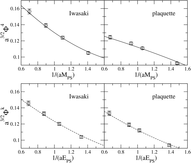
Figure 11: Charmed-strange pseudoscalar meson decay constants obtained from the temporal(top) and spatial(bottom) components of the axial vector current as a function of $aM_{PS}$ in case of $\kappa_{light}=\kappa_{3}$.

where ${Z_{A^{\rm impr}_{\bf 4}}}$ and ${Z_{A^{\rm impr}_{\bf k}}}$ are the decay matrix elements defined in Eq.(27). Note that only the improved axial vector current with $c_{A_{\mu}}^{\rm PT+NP}$ is considered for the plaquette gauge action. In Fig.11 we plot $a^{3/2}\Phi_{P}^{4}$ and $a^{3/2}\Phi_{P}^{k}$ as a function of $1/(aM_{PS}^{\rm pole,kin})$. The interpolation lines are obtained by fitting the results with the following ansatz:

$$a^{3/2}\Phi_{PS}^{4} = A+B/(aM_{PS}^{\rm pole,kin})+C/(aM_{PS}^{\rm pole,kin})^{2}+Dam_{q}^{light},$$ (39)

$$a^{3/2}\Phi_{PS}^{k} = A+B/(aE_{PS}^{\rm pole,kin})+C/(aE_{PS}^{\rm pole,kin})^{2}+Dam_{q}^{light}.$$ (40)

Using the fitted values of the parameters in Table 10-11, we obtain $f_{D_{s}}$ in physical unit. Table 12 lists the results of $f_{PS}$ at $\kappa_{c}(D_{s},M^{\rm pole})$ and $\kappa_{s}$ and $f_{PS}$ at $\kappa_{c}(D_{s},M^{\rm kin})$ and $\kappa_{s}$ for each gauge action together with the experimental value.

IV.3 Cutoff effects

We now consider the cutoff effects in our results. Leading cutoff effects for the gauge part are $O(a^{2}{\Lambda}_{\rm QCD}^{2})$. The light quark action also has $O(a^{2}{\Lambda}_{\rm QCD}^{2})$ errors, since the nonperturbative value of $c_{\rm SW}$ is employed for each gauge action. For the RHQ action, on the other hand, the leading cutoff effects are $O(\alpha_{s}(\mu)^{2}f_{0}^{(2)}(am_{Q}))$ with $\alpha_{s}(\mu)=g^{2}(\mu)/(4\pi)$, which comes from the fact that the parameter $\nu$ associated with the $O(1)$ kinetic term is only adjusted up to one-loop level. Since this error is responsible for the deviation of $c_{\rm eff}$ from unity, the mass dependence of $c_{\rm eff}$ shown in Figs.4 and 5 tells us that $f_{0}^{(2)}(m_{Q}a)$ is a smooth function of $am_{Q}$ in the range of the heavy quark mass employed in our simulation. In addition, there exists the $O(\alpha_{s}(\mu)^{2}g_{0}^{(2)}(am_{Q}))$ errors originating from the heavy quark axial vector currents whose renormalization factors are determined up to one-loop level. These are the leading cutoff effects in the deviation of $R$ from unity shown in Fig.6, where we find fairly smooth $am_{Q}$ dependence.

Let us take into account these $O(\alpha_{s}(\mu)^{2}f_{0}^{(2)}(am_{Q}),\alpha_{s}(\mu)^{2}g_{0}^{(2)}(am_{Q}))$ effects in our error estimate using a difference of the charmed meson hyperfine splittings obtained with $M_{\rm pole}$ and $M_{\rm kin}$ and also a difference of the charmed meson decay constants extracted from $A_{k}$ and $A_{4}$. For the hyperfine splittings we take the pole mass result as the central value and a difference between two results as a systematic error. In Table 13 our final result for the charmonium hyperfine splitting in physical unit is also presented, where the central value is $\Delta M_{\rm pole}(J/\psi-\eta_{c})$, the first error is statistical and the second is a systematic error explained above. The second error, much larger than the first, is about $16\%$ for the Iwasaki action and about $12\%$ for the plaquette action. Similarly, our final result for the charmed-strange meson hyperfine splitting in physical unit is given in Table13, where the central value is $\Delta M_{\rm pole}(D_{s}^{*}-D_{s})$, the first error is statistical and the second is a systematic error. It is interesting that the second errors for the charmed-strange meson hyperfine splitting , which are about $8\%$ for the Iwasaki action and about $7\%$ for the plaquette action, are half of those for the charmonium hyperfine splitting. This suggests that the dominant systematic errors come from the heavy quarks, so that they are proportional to a number of heavy quarks in the mesons. In Table 13 our final result for the $D_{s}$ meson decay constant in physical unit is also presented, where we take $f_{D_{s}}(A_{4})$ with $M_{\rm pole}$ as the central value. The first error is statistical and the second and the third are systematic errors estimated from a difference of $f_{D_{s}}(A_{4})$ between $M_{\rm pole}$ and $M_{\rm kin}$ and a difference between $f_{D_{s}}(A_{4})$ and $f_{D_{s}}(A_{k})$ with $M_{\rm pole}$, respectively. Both the second and third errors are less than $1\%$ for the plaquette gauge action. For the Iwasaki gauge action, on the other hand, the third error is about $5\%$ though less than $1\%$ for the second. Smallness of the third error for the plaquette action may be partly due to the use of $c_{A}^{\rm PT+NP}$. Note that the systematic errors associated with the heavy quark action are estimated at one lattice spacing in this paper. Therefore, in future works, it is desirable to study these systematic errors by changing the lattice spacing.

Once the systematic errors are taken into account, our results of the hyperfine splitting for two gauge actions agree with each other. For $f_{D_{s}}$, on the other hand, an agreement is not so excellent: the difference is still 1.5$\sigma$ even if we take the systematic error for the Iwasaki action. It could be interesting to see whether the difference diminishes if we employ $c_{A}^{\rm PT+NP}$ for the Iwasaki gauge action.

IV.4 Comparison with the previous results

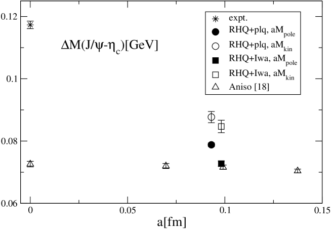
Figure 12: Comparison of charmonium S-state hyperfine splitting in physical unit.

In Fig.12 our results of the S-state charmonium hyperfine splitting are compared with a previous result obtained by the CP-PACS collaboration using the anisotropic lattice QCDAniso:CC:Spctrm , where the effective speed of light is nonperturbatively adjusted to unity such that $M^{\rm pole}=M^{\rm kin}$. Both results are plotted as a function of the lattice spacing determined by the Sommer scale $r_{0}=0.5$fm. Our result with the pole mass for the Iwasaki gauge action is consistent with the continuum limit of the anisotropic lattice result within the small statistical error, though the kinetic mass result is rather large. For the plaquette gauge action, on the other hand, both the pole and kinetic mass results are larger than the anisotropic lattice results. The large systematic error due to the pole to kinetic mass difference should be eliminated with the use of nonperturbative $\nu$ in future calculations. It should be noted that all the results are smaller than the experimental value by about $40\%$.

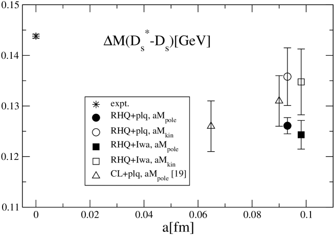
Figure 13: Comparison of $D_{s}$ meson hyperfine splitting in physical unit. The results of Ref.fDs.UKQCD are slightly shifted in $a$ coordinate for visibility.

Figure 13 shows the comparison of our results of the S-state charmed-strange meson hyperfine splitting with a previous result obtained by the UKQCD collaboration using the heavy clover quark actionfDs.UKQCD . We observe that all the results agree within large statistical errors, though they are smaller than the experimental value by about $10\%$.

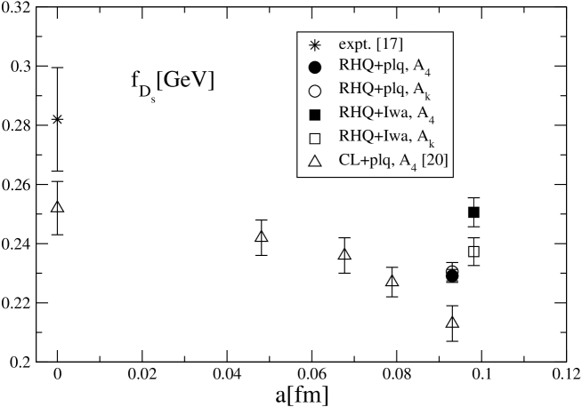
Figure 14: Comparison of $D_{s}$ meson decay constant in physical unit.

In Fig.14 we compare our results of $f_{D_{s}}$ with a previous result obtained by the ALPHA collaboration using the heavy clover quark and the plaquette gauge actionsfDs.ALPHA . Our results at finite lattice spacing are closer to the ALPHA result at the continuum limit than at a similar lattice spacing. This could indicate that $f_{D_{s}}$ from the RHQ action has a good scaling behavior, which should be checked in future scaling studies. We also point out that $c_{A}^{\rm PT+NP}$ for the Iwasaki gauge action may reduce the difference between $f_{D_{s}}(A_{4})$ and $f_{D_{s}}(A_{k})$. We also leave it to future work.

V Conclusion

We have carried out a first nonperturbative test of the RHQ action focusing on the magnitude of the cutoff errors. We investigate the dispersion relation of the pseudo-scalar meson and the space-time symmetry for the pseudo-scalar meson decay matrix element. Our results show that the RHQ action has much smaller cutoff errors than the heavy clover quark action around the charm quark mass.

We also investigate the systematic errors due to the cutoff effects for the physical observables. In case of the charmonium (charmed-strange) hyperfine splitting, a difference between the results with $M^{\rm pole}$ and $M^{\rm kin}$ is used to estimate the systematic error, which is as large as $16\%$ ($8\%$) for the Iwasaki gauge action and $12\%$ ($7\%$) for the plaquette gauge action. For the $D_{s}$ meson decay constant $f_{D_{s}}$, we estimate the systematic error by a difference between $f_{D_{s}}(A_{4})$ and $f_{D_{s}}(A_{k})$ as well as a difference between $M^{\rm pole}$ and $M^{\rm kin}$. The latter is negligible for both gauge actions, while the former is about $5\%$ for the Iwasaki gauge action and $0.5\%$ for the plaquette gauge action.

There are two important subjects for future studies. One is a further improvement of the RHQ action to reduce the cutoff effects. In particular, it is rather easy to tune the improvement coefficient $\nu$ nonperturbatively, which is supposed to eliminate the leading $O(\alpha_{s}^{2})$ errors. This study is under waylatt05 . The other is the inclusion of light dynamical quark effects. It is interesting to investigate whether the deficit in the quenched value for the S-state charmonium hyperfine splitting is fully accounted by the sea quark effects.

Appendix A Renormalization factors and improvement coefficients for massive quarks

In this appendix we explain how to determine the input parameters for the RHQ action and the axial vector currents in our numerical simulation, such as $\kappa$, the improvement coefficients and the renormalization factors together with the mean field improvement discussed in Refs.cEcB ; zAcA .

The mean field improvement is introduced as the redefinition of link variable $U_{\mu}(x)\rightarrow u_{0}(U_{\mu}(x)/u_{0})\equiv u_{0}\tilde{U}_{\mu}(x)$, where $u_{0}=P^{1/4}$ with the averaged plaquette value $P$ in our simulation. The one-loop expression for $u_{0}$ is given by

$$u_{0}=1-g^{2}\frac{C_{F}}{2}T_{\rm MF},$$ (41)

where $T_{\rm MF}=1/8$ for the plaquette gauge action and $0.0525664$ for the Iwasaki gauge actionTadpole.val .

With the replacement $U_{\mu}(x)\rightarrow u_{0}\tilde{U}_{\mu}(x)$ it is natural to introduce the boosted gauge coupling $g_{0}^{2}/u_{0}^{4}$, which is related to the ${\overline{\rm MS}}$ coupling constant $g_{{\overline{\rm MS}}}^{2}(\mu)$ with the scale $\mu=1/a$ as

$$\frac{1}{g^{2}_{\overline{\rm MS}}(\mu)}=\frac{c_{0}P+8c_{1}R}{g_{0}^{2}}-0.1006+0.03149N_{f}+\frac{11-\frac{2}{3}N_{f}}{8\pi^{2}}{\rm log}(a\mu)$$ (42)

for the Iwasaki gauge action and the $O(a)$ improved Wilson quark actionCP-PACS:fHL:NRQCD:Nf=2 , and

$$\frac{1}{g^{2}_{\overline{\rm MS}}(\mu)}=\frac{P}{g_{0}^{2}}-0.1349+0.03149N_{f}+\frac{11-\frac{2}{3}N_{f}}{8\pi^{2}}{\rm log}(a\mu)$$ (43)

for the plaquette gauge action and the $O(a)$ improved Wilson quark actiongmass . In the following we simply use $g^{2}$ to express $g_{{\overline{\rm MS}}}^{2}(\mu=1/a)$.

The inverse quark propagator at the leading order without the mean-field improvement is given by

$$aS_{q}^{-1} = am_{0}+g^{2}am_{c}^{(1)}+i\gamma_{4}\sin(p_{4}a)+i\nu\sum_{k}\gamma_{k}\sin(p_{k}a)+r_{t}(1-\cos(p_{4}a))+r_{s}\sum_{k}(1-\cos(p_{k}a))$$ (44)

where $am_{0}$ is the bare quark mass appeared in the action. Note that we include the one-loop contribution to the critical quark mass, $g^{2}m_{c}^{(1)}$, in the leading order. A reason for this will become clear later. The pole mass $a{m_{p}^{(0)}}$, determined from the zero of the inverse propagator by setting $p_{4}=i{m_{p}^{(0)}}$ and $p_{k}=0$, satisfies

$$\sinh(a{m_{p}^{(0)}})+r_{t}\cosh(a{m_{p}^{(0)}})=am+r_{t},$$ (45)

where $am$ is a shifted quark mass defined by $am=am_{0}+ag^{2}m_{c}^{(1)}$. If we perform the replacement $U_{\mu}(x)\rightarrow u_{0}\tilde{U}_{\mu}(x)$ in the RHQ action given in Eq.(I) or Eq.(3), the inverse quark propagator at the leading order with the mean-field improvement becomes

$$a\tilde{S}_{q}^{-1} = am_{0}+g^{2}a\Delta m_{c}^{(1)}+i\gamma_{4}u_{0}\sin(p_{4}a)+i\nu\sum_{k}\gamma_{k}u_{0}\sin(p_{k}a)+r_{t}(1-u_{0}\cos(p_{4}a))+r_{s}\sum_{k}(1-u_{0}\cos(p_{k}a))$$

where $g^{2}a\Delta m_{c}^{(1)}=g^{2}am_{c}^{(1)}-(r_{t}+3r_{s})(1-u_{0})$. Then the pole mass $a{{\tilde{m}_{p}}^{(0)}}$ at the tree-level with the mean-field improvement satisfies

$$u_{0}\sinh(a{{\tilde{m}_{p}}^{(0)}}) = am_{0}+ag^{2}\Delta m_{c}^{(1)}+r_{t}(1-u_{0}\cosh(a{{\tilde{m}_{p}}^{(0)}}))+3r_{s}(a{{\tilde{m}_{p}}^{(0)}})(1-u_{0})$$ (47)

$$= am+r_{t}u_{0}(1-\cosh(a{{\tilde{m}_{p}}^{(0)}}))+(1-u_{0})3(r_{s}(a{{\tilde{m}_{p}}^{(0)}})-1).$$

Note that the shifted quark mass $am$ is kept equal with and without the mean field improvement. Therefore both ${m_{p}^{(0)}}$ and ${{\tilde{m}_{p}}^{(0)}}$ vanish at $am=0$. Since the remaining one-loop correction to the quark mass is multiplicative to $m$, the pole masses in both definitions vanish at $am=0$ also at one-loop level. The inclusion of $g^{2}am_{c}^{(1)}$ or $g^{2}a\Delta m_{c}^{(1)}$ at leading order is necessary to satisfy this property. Although in this work we follow the mean-field improvement procedure given in Sec.6 of Ref.cEcB which does not include the $\Delta m_{c}$ correction, the effects on the improvement parameters are less than 1%. Eqs.(45) and (47) lead to the following relation that

$$a{m_{p}^{(0)}} = a{{\tilde{m}_{p}}^{(0)}}+(u_{0}-1)\frac{\sinh(a{{\tilde{m}_{p}}^{(0)}})+r_{t}(\cosh(a{{\tilde{m}_{p}}^{(0)}})-1)+3(r_{s}(a{{\tilde{m}_{p}}^{(0)}})-1)}{\cosh(a{{\tilde{m}_{p}}^{(0)}})+r_{t}\sinh(a{{\tilde{m}_{p}}^{(0)}})}$$ (48)

$$\equiv {a{{\tilde{m}_{p}}^{(0)}}}+g^{2}a\Delta m_{p},$$

where

$$a\Delta m_{p} = -\frac{C_{F}}{2}T_{\rm MF}\frac{\sinh(a{{\tilde{m}_{p}}^{(0)}})+r_{t}(\cosh(a{{\tilde{m}_{p}}^{(0)}})-1)+3(r_{s}(a{{\tilde{m}_{p}}^{(0)}})-1)}{\cosh(a{{\tilde{m}_{p}}^{(0)}})+r_{t}\sinh(a{{\tilde{m}_{p}}^{(0)}})}.$$ (49)

As a consequence, the quark pole mass is written at the one-loop level as

$$am_{p}=a{m_{p}^{(0)}}+g^{2}am_{p}^{(1)}={a{{\tilde{m}_{p}}^{(0)}}}+g^{2}a\tilde{m}_{p}^{(1)},$$ (50)

where $a\tilde{m}_{p}^{(1)}=am_{p}^{(1)}+a\Delta m_{p}$, and $am_{p}^{(1)}$ is the one-loop correction to the pole mass without the mean field improvementcEcB .

The mean-field improved parameters $Z_{q}$, $\nu$, $r_{s}$, $c_{E}$ and $c_{B}$ are given below with the use of $a{{\tilde{m}_{p}}^{(0)}}$ and $a\tilde{m}_{p}^{(1)}$:

$$Z_{q,{\rm latt}}(a{{\tilde{m}_{p}}^{(0)}}) = Z_{q,{\rm latt}}^{(0)}u_{0}\left(1+g^{2}\frac{Z_{q,{\rm latt}}^{(1)}}{Z_{q,{\rm latt}}^{(0)}}+g^{2}\frac{C_{F}}{2}T_{\rm MF}+\frac{g^{2}}{Z_{q,{\rm latt}}^{(0)}}\frac{\partial Z_{q,{\rm latt}}^{(0)}}{\partial{m_{p}^{(0)}}}{a\Delta m_{p}}\right),$$ (51)

$$\nu(a{{\tilde{m}_{p}}^{(0)}}) = \nu^{(0)}+g^{2}\nu^{(1)}+g^{2}\frac{\partial\nu^{(0)}}{\partial a{m_{p}^{(0)}}}{a\Delta m_{p}},$$ (52)

$$r_{s}(a{{\tilde{m}_{p}}^{(0)}}) = r_{s}^{(0)}+g^{2}r_{s}^{(1)}+g^{2}\frac{\partial r_{s}^{(0)}}{\partial a{m_{p}^{(0)}}}{a\Delta m_{p}},$$ (53)

$${\it c}_{\it E}(a{{\tilde{m}_{p}}^{(0)}}) = {\it c}_{\it E}^{(0)}\frac{1}{u_{0}^{3}}\left(1+g^{2}\frac{{\it c}_{\it E}^{(1)}}{{\it c}_{\it E}^{(0)}}-g^{2}\frac{3}{2}C_{F}T_{\rm MF}+\frac{g^{2}}{{\it c}_{\it E}^{(0)}}\frac{\partial{\it c}_{\it E}^{(0)}}{\partial{m_{p}^{(0)}}}{a\Delta m_{p}}\right),$$ (54)

$${\it c}_{\it B}(a{{\tilde{m}_{p}}^{(0)}}) = {\it c}_{\it B}^{(0)}\frac{1}{u_{0}^{3}}\left(1+g^{2}\frac{{\it c}_{\it B}^{(1)}}{{\it c}_{\it B}^{(0)}}-g^{2}\frac{3}{2}C_{F}T_{\rm MF}+\frac{g^{2}}{{\it c}_{\it B}^{(0)}}\frac{\partial{\it c}_{\it B}^{(0)}}{\partial{m_{p}^{(0)}}}{a\Delta m_{p}}\right),$$ (55)

where one-loop corrections, $Z_{q,{\rm latt}}^{(1)}$, $\nu^{(1)}$, $r_{s}^{(1)}$, ${\it c}_{\it E}^{(1)}$ and ${\it c}_{\it B}^{(1)}$, have already been calculated in ref. cEcB . We replace a perturbative value of $u_{0}$ in the above expressions by $u_{0}=P^{1/4}$ with $P$ taken from our simulation. We finally determine $\kappa$ in terms of ${{\tilde{m}_{p}}^{(0)}}$ as follows. Using the relation of Eq.(47) with $r_{t}=1$

$$am_{0}+a\Delta m_{c}=u_{0}e^{a{{\tilde{m}_{p}}^{(0)}}}-1-3r_{s}(1-u_{0}),$$ (56)

the hopping parameter $\kappa$ is given in terms of ${{\tilde{m}_{p}}^{(0)}}$:

$$\kappa\equiv\frac{1}{2}\frac{1}{1+3r_{s}+am_{0}}=\frac{1}{2}\frac{1}{u_{0}(e^{a{{\tilde{m}_{p}}^{(0)}}}+3r_{s})-a\Delta m_{c}}.$$ (57)

With this definition, $\kappa$ becomes $\kappa_{crit}$ at the one-loop level for $a{{\tilde{m}_{p}}^{(0)}}=0$.

In a similar manner we can derive the renormalization factor and the $O(a)$ improvement coefficients for the axial-vector currents in Eq.(9). The matching factor $Z_{A_{\mu}}$ from the lattice to the continuum ${\overline{\rm MS}}$ scheme is given in Ref.zAcA :

$$Z_{A_{\mu}}=\frac{Z_{A_{\mu}}^{\rm latt}}{Z_{A_{\mu}}^{{\overline{\rm MS}}}} = \sqrt{Z_{Q,{\rm latt}}^{(0)}(a{{\tilde{m}_{p1}}^{(0)}})}\sqrt{Z_{q,{\rm latt}}^{(0)}(a{{\tilde{m}_{p2}}^{(0)}})}u_{0}\left(1-g^{2}\Delta_{A_{\mu}}\right.$$ (58)

$$\left.+g^{2}\frac{C_{F}}{2}T_{\rm MF}+\frac{1}{2}\frac{g^{2}}{Z_{Q,{\rm latt}}^{(0)}}\frac{\partial Z_{Q,{\rm latt}}^{(0)}}{\partial{m_{p1}^{(0)}}}{a\Delta{m_{p1}}}+\frac{1}{2}\frac{g^{2}}{Z_{q,{\rm latt}}^{(0)}}\frac{\partial Z_{q,{\rm latt}}^{(0)}}{\partial{m_{p2}^{(0)}}}{a\Delta{m_{p2}}}\right),$$

where $\Delta_{A_{\mu}}$ is the one-loop correction to the renormalization factor of $A_{\mu}$zAcA . For the $O(a)$ improvement coefficients, on the other hand, we use the expressions of Eq.(9) suitable for our numerical simulations, which are related to those in Ref.zAcA as

$$c_{A_{k}}^{+} = g^{2}c_{A_{k}}^{+,{\rm PT}},$$ (59)

$$c_{A_{4}}^{+} = g^{2}c_{A_{4}}^{+,{\rm PT}}(a{{\tilde{m}_{q}}^{(0)}}+a{{\tilde{m}_{Q}}^{(0)}})/{\rm sinh}(a{{\tilde{m}_{q}}^{(0)}}+a{{\tilde{m}_{Q}}^{(0)}}),$$ (60)

$$c_{A_{\mu}}^{-} = g^{2}c_{A_{\mu}}^{-,{\rm PT}}/u_{0},$$ (61)

$$c_{A_{\mu}}^{L} = -g^{2}c_{A_{\mu}}^{L,{\rm PT}}/u_{0},$$ (62)

$$c_{A_{\mu}}^{R} = g^{2}c_{A_{\mu}}^{R,{\rm PT}}/u_{0},$$ (63)

where $c_{A_{\mu}}^{\{\pm,L,R\},{\rm PT}}$ are calculated as a function of ${{\tilde{m}_{Q}}^{(0)}}$ and the superscript PT represents that these parameters are defined in Ref.zAcA . Note in particular that a minus sign in the relation (62). A factor $1/u_{0}$ in Eqs.(61)$-$(63) is due to link variables in the point splitting operators of Eqs.(10) and (11). In Eq.(60) we multiply an extra factor $({{\tilde{m}_{q}}^{(0)}}+{{\tilde{m}_{Q}}^{(0)}})/{\rm sinh}({{\tilde{m}_{q}}^{(0)}}+{{\tilde{m}_{Q}}^{(0)}})$ since $c_{A_{4}}^{+,{\rm PT}}$ in Ref.zAcA is a coefficient of $({{\tilde{m}_{q}}^{(0)}}+{{\tilde{m}_{Q}}^{(0)}})\bar{q}(q)Q(p)$ while $c_{A_{4}}^{+}$ in Eq.(9) is a coefficient ${\rm sinh}({{\tilde{m}_{q}}^{(0)}}+{{\tilde{m}_{Q}}^{(0)}})\bar{q}(q)Q(p)$.

Table 1: Simulation parameters for the RHQ action with the Iwasaki gauge action(upper) and the plaquette gauge action(lower).

	Iwasaki
	flavor	$\kappa$	$M_{PS}/M_{V}$	$\nu$	$r_{s}$	$c_{B}$	$\omega=c_{E}/c_{B}$
	$\kappa_{1}$	$0.13295$	$0.5567(36)$	$1.0$	$1.0$	$1.50$	$1.0$
light	$\kappa_{2}$	$0.13222$	$0.6898(23)$	$1.0$	$1.0$	$1.50$	$1.0$
	$\kappa_{3}$	$0.13138$	$0.7734(16)$	$1.0$	$1.0$	$1.50$	$1.0$
	$\kappa_{4}$	$0.11513$	$0.9372(7)$	$1.03160$	$1.12787$	$1.66304$	$0.92064$
heavy	$\kappa_{5}$	$0.10524$	$0.9680(4)$	$1.05935$	$1.20160$	$1.75930$	$0.88889$
	$\kappa_{6}$	$0.09455$	$0.9813(2)$	$1.10040$	$1.29777$	$1.88490$	$0.85628$
	$\kappa_{7}$	$0.07841$	$0.9901(1)$	$1.19159$	$1.48857$	$2.13426$	$0.81003$
	plaquette
	flavor	$\kappa$	$M_{PS}/M_{V}$	$\nu$	$r_{s}$	$c_{B}$	$\omega=c_{E}/c_{B}$
	$\kappa_{1}$	$0.13449$	$0.5492(173)$	$1.0$	$1.0$	$1.769$	$1.0$
light	$\kappa_{2}$	$0.13373$	$0.7088(27)$	$1.0$	$1.0$	$1.769$	$1.0$
	$\kappa_{3}$	$0.13298$	$0.7837(16)$	$1.0$	$1.0$	$1.769$	$1.0$
	$\kappa_{4}$	$0.11456$	$0.9345(5)$	$1.04161$	$1.16034$	$2.02423$	$0.91709$
heavy	$\kappa_{5}$	$0.10190$	$0.9728(2)$	$1.08301$	$1.26201$	$2.17790$	$0.88345$
	$\kappa_{6}$	$0.09495$	$0.9808(2)$	$1.11284$	$1.32840$	$2.27776$	$0.86586$
	$\kappa_{7}$	$0.07490$	$0.9911(1)$	$1.23871$	$1.58259$	$2.66050$	$0.81742$

Table 2: Simulation parameters for the heavy clover quark action with the Iwasaki gauge action(upper) and the plaquette gauge action(lower).

	Iwasaki
	flavor	$\kappa$	$M_{PS}/M_{V}$	$\nu$	$r_{s}$	$c_{B}$	$\omega=c_{E}/c_{B}$
light	$\kappa_{3}$	$0.13138$	$0.7734(16)$	$1.0$	$1.0$	$1.50$	$1.0$
	$\tilde{\kappa}_{4}$	$0.1256$	$0.9353(5)$	$1.0$	$1.0$	$1.50$	$1.0$
heavy	$\tilde{\kappa}_{5}$	$0.1186$	$0.9717(3)$	$1.0$	$1.0$	$1.50$	$1.0$
	$\tilde{\kappa}_{6}$	$0.1119$	$0.9836(2)$	$1.0$	$1.0$	$1.50$	$1.0$
	plaquette
	flavor	$\kappa$	$M_{PS}/M_{V}$	$\nu$	$r_{s}$	$c_{B}$	$\omega=c_{E}/c_{B}$
light	$\kappa_{3}$	$0.13298$	$0.7837(16)$	$1.0$	$1.0$	$1.769$	$1.0$
	$\tilde{\kappa}_{4}$	$0.12780$	$0.9359(8)$	$1.0$	$1.0$	$1.769$	$1.0$
heavy	$\tilde{\kappa}_{5}$	$0.11900$	$0.9770(3)$	$1.0$	$1.0$	$1.769$	$1.0$
	$\tilde{\kappa}_{6}$	$0.11480$	$0.9834(2)$	$1.0$	$1.0$	$1.769$	$1.0$

Table 3: Smearing parameters.

action	Iwasaki+RHQ			Iwasaki+CL			plaquette+RHQ			plaquette+CL
	flavor	$A$	$B$	flavor	$A$	$B$	flavor	$A$	$B$	flavor	$A$	$B$
	$\kappa_{1}$	$1.28$	$0.28$				$\kappa_{1}$	$1.28$	$0.35$
light	$\kappa_{2}$	$1.25$	$0.3$				$\kappa_{2}$	$1.28$	$0.35$
	$\kappa_{3}$	$1.25$	$0.32$	$\kappa_{3}$	$1.25$	$0.32$	$\kappa_{3}$	$1.28$	$0.35$	$\kappa_{3}$	$1.28$	$0.35$
	$\kappa_{4}$	$1.25$	$0.50$	$\tilde{\kappa}_{4}$	$1.25$	$0.50$	$\kappa_{4}$	$1.25$	$0.50$	$\tilde{\kappa}_{4}$	$1.25$	$0.50$
heavy	$\kappa_{5}$	$1.25$	$0.58$	$\tilde{\kappa}_{5}$	$1.25$	$0.65$	$\kappa_{5}$	$1.25$	$0.58$	$\tilde{\kappa}_{5}$	$1.25$	$0.65$
	$\kappa_{6}$	$1.25$	$0.65$	$\tilde{\kappa}_{6}$	$1.25$	$0.82$	$\kappa_{6}$	$1.25$	$0.60$	$\tilde{\kappa}_{6}$	$1.25$	$0.65$
	$\kappa_{7}$	$1.25$	$1.00$				$\kappa_{7}$	$1.25$	$0.8$

Table 4: Fitting range from $t_{\rm min}$ to $t_{\rm max}$ for the two-point functions.

			Iwasaki	plaquette
correlator	system	source	$t_{\rm min}/t_{\rm max}$	$t_{\rm min}/t_{\rm max}$
$\langle VV^{\dagger}\rangle$	H-L	S	10/22	7/17
$\langle PP^{\dagger}\rangle$	H-L	S	10/22	9/22
$\langle PP^{\dagger}\rangle$	H-L	P	13/22	14/22
$\langle PP^{\dagger}\rangle$ with $|{\vec{p}}|\neq 0$	H-L	S	8/20	9/22
$\langle VV^{\dagger}\rangle$	H-H	S	12/22	11/21
$\langle PP^{\dagger}\rangle$	H-H	S	12/22	11/21
$\langle PP^{\dagger}\rangle$	H-H	P	16/22	18/23
$\langle PP^{\dagger}\rangle$ with $|{\vec{p}}|\neq 0$	H-H	S	12/20	10/22

Table 5: Fitting results for chiral extrapolation of $M_{PS}^{2}$ for the light-light pseudoscalar meson.

action	$A$	$\kappa_{crit}$	$\chi^{2}$/dof
Iwasaki+RHQ	$0.7583(15)$	$0.133802(4)$	$6.3$
plaquette+RHQ	$0.7886(38)$	$0.135247(9)$	$0.7$

Table 6: Hopping parameters at the physical points.

action	$\kappa_{ud}$	$\kappa_{s}(K)$	$\kappa_{c}(J/\psi,M_{\rm pole})$	$\kappa_{c}(J/\psi,M_{\rm kin})$	$\kappa_{c}(D_{s},M_{\rm pole})$	$\kappa_{c}(D_{s},M_{\rm kin})$
Iwasaki+RHQ	$0.133749(4)$	$0.132422(4)$	$0.099414(22)$	$0.102362(377)$	$0.099640(49)$	$0.101528(862)$
plaquette+RHQ	$0.135200(9)$	$0.134026(5)$	$0.100593(21)$	$0.102610(343)$	$0.100669(35)$	$0.102402(810)$

Table 7: Fitting results for the heavy-heavy hyperfine splitting as a function of the vector meson mass.

	$M_{\rm pole}$				$M_{\rm kin}$
action	$A$	$B$	$C$	$\chi^{2}$/dof	$A$	$B$	$C$	$\chi^{2}$/dof
Iwasaki+RHQ	$0.0452(14)$	$0.0156(43)$	$0.0009(26)$	$0.0018$	$0.0676(23)$	$-0.0120(78)$	$0.0122(50)$	$0.001$
plaquette+RHQ	$0.0524(14)$	$-0.0028(33)$	$0.0081(19)$	$0.03$	$0.0745(20)$	$-0.0403(59)$	$0.0288(34)$	$0.10$

Table 8: Charmonium and charmed-strange meson hyper-fine splittings in unit of GeV with $M_{\rm pole}$ and $M_{\rm kin}$. The lattice spacing is determined by the Sommer scale $r_{0}=0.5$fm.

	Iwasaki		plaquette
	$M_{\rm pole}$	$M_{\rm kin}$	$M_{\rm pole}$	$M_{\rm kin}$	expt.
$\Delta M(J/\psi-\eta_{c})$	$0.0728(8)$	$0.0847(20)$	$0.0788(6)$	$0.0877(18)$	$0.1173(12)$
$\Delta M(D_{s}^{*}-D_{s})$	$0.1243(28)$	$0.1348(65)$	$0.1261(16)$	$0.1358(57)$	$0.1438(4)$

Table 9: Fitting results for the heavy-light hyperfine splitting as a function of the pseudoscalar meson mass.

	$M_{\rm pole}$				$M_{\rm kin}$
action	$A$	$B$	$C$	$\chi^{2}$/dof	$A$	$B$	$C$	$\chi^{2}$/dof
Iwasaki+RHQ	$0.0602(35)$	$0.0028(17)$	$-0.0628(167)$	$0.13$	$0.0649(75)$	$0.0012(41)$	$-0.0106(337)$	$0.03$
plaquette+RHQ	$0.0545(20)$	$0.0022(10)$	$-0.0523(121)$	$0.22$	$0.0549(70)$	$0.0049(36)$	$-0.0224(497)$	$0.61$

Table 10: Fitting results for the heavy-light pseudoscalar meson decay constant determined from $A_{4}$ as a function of the pseudoscalar meson mass.

	$M_{\rm pole}$
action	$A$	$B$	$C$	$D$	$\chi^{2}$/dof
Iwasaki+RHQ	$0.2204(93)$	$-0.1337(113)$	$0.0312(39)$	$0.1780(199)$	$0.43$
plaquette+RHQ	$0.1285(20)$	$-0.0217(26)$	$-0.0065(10)$	$0.1967(140)$	$2.9$
	$M_{\rm kin}$
action	$A$	$B$	$C$	$D$	$\chi^{2}$/dof
Iwasaki+RHQ	$0.2275(96)$	$-0.1470(127)$	$0.0368(47)$	$0.1820(210)$	$0.33$
plaquette+RHQ	$0.1326(29)$	$-0.0241(49)$	$-0.0071(22)$	$0.1903(131)$	$1.7$

Table 11: Fitting results for the heavy-light pseudoscalar meson decay constant determined from $A_{k}$ as a function of the pseudoscalar meson mass.

	$M_{\rm pole}$
action	$A$	$B$	$C$	$D$	$\chi^{2}$/dof
Iwasaki+RHQ	$0.1892(88)$	$-0.0955(110)$	$0.0174(39)$	$0.1788(190)$	$0.44$
plaquette+RHQ	$0.1709(57)$	$-0.0811(73)$	$0.0144(27)$	$0.1338(306)$	$0.55$
	$M_{\rm kin}$
action	$A$	$B$	$C$	$D$	$\chi^{2}$/dof
Iwasaki+RHQ	$0.1975(96)$	$-0.1104(129)$	$0.0235(50)$	$0.1836(198)$	$0.29$
plaquette+RHQ	$0.1746(54)$	$-0.0868(70)$	$0.0163(28)$	$0.1370(311)$	$0.86$

Table 12: $D_{s}$ meson decay constants in unit of GeV determined from $A_{k}$ and $A_{4}$ using $M_{\rm pole}$ as well as $M_{\rm kin}$. The lattice spacing is determined by the Sommer scale $r_{0}=0.5$fm. The experimental value for $f_{D_{s}}$ is take from Ref.fDs_expt .

	Iwasaki		plaquette
	$M_{\rm pole}$	$M_{\rm kin}$	$M_{\rm pole}$	$M_{\rm kin}$	expt.
$f_{D_{s}}(A_{4})$	$0.2506(49)$	$0.2496(48)$	$0.2291(22)$	$0.2304(24)$	$0.282(16)(7)$
$f_{D_{s}}(A_{k})$	$0.2373(47)$	$0.2369(46)$	$0.2305(31)$	$0.2304(30)$	$0.282(16)(7)$

Table 13: The final results of the charmonium hyperfine mass splitting, the charmed-strange meson hyperfine splitting and the $D_{s}$ meson decay constant in unit of GeV. The first error is statistical and the second and the third ones are the cutoff errors explained in the text. The lattice spacing is determined by the Sommer scale $r_{0}=0.5$fm.

	Iwasaki	plaquette	expt.
$\Delta M(J/\Psi-\eta_{c})$	$0.0728(8)(_{-0}^{+119})$	$0.0788(6)(_{-0}^{+89})$	$0.1173(12)$
$\Delta M(D_{s}^{*}-D_{s})$	$0.1243(28)(_{-0}^{+105})$	$0.1261(16)(_{-0}^{+97})$	$0.1438(4)$
$f_{D_{s}}(A_{4})$	$0.2506(49)(_{-0}^{+10})(_{-0}^{+133})$	$0.2291(22)(_{-0}^{+13})(_{-0}^{+14})$	$0.267(33)$

References

- (1) S. Aoki, Y. Kuramashi and S. Tominaga, Prog. Theor. Phys. 109 (2003) 383.
- (2) K. Symanzik, in Mathematical Problems In Theoretical Physics, eds. R. Schrader et al., Lecture Notes in Physics, Vol. 153 (Springer, New York, 1982).
- (3) K. Symanzik, Nucl. Phys. B226 (1983), 187; 205.
- (4) B. Sheikholeslami and R. Wohlert, Nucl. Phys. B259 (1985), 572.
- (5) M. Lüscher, S. Sint, R. Sommer and P. Weisz Nucl. Phys. B478 (1996), 365.
- (6) M. Lüscher and P. Weisz, Commun. Math. Phys. 97 (1985), 59.
- (7) N. H. Christ, M. Li, H.-W. Lin, hep-lat/0608006; H.-W. Lin, and N. H. Christ, hep-lat/0608005.
- (8) S. Aoki, Y. Kayaba and Y. Kuramashi, Nucl. Phys. B 697 (2004) 271.
- (9) S. Aoki, Y. Kayaba and Y. Kuramashi, Nucl. Phys. B 689 (2004) 127.
- (10) S. Aoki, Y. Kayaba, Y. Kuramashi and N. Yamada, hep-lat/0409001, to appear in Progress of Theoretical Physics Supplement.
- (11) Y. Iwasaki, preprint, UTHEP-118 (Dec. 1983), unpublished.
- (12) S. Necco, Nucl. Phys. B 683 (2004) 137.
- (13) M. Guagnelli, R. Sommer, H. Wittig, Nucl. Phys. B 535 (1998) 389.
- (14) CP-PACS and JLQCD Collaborations: S. Aoki et al., Phys. Rev. D73 (2006) 034501.
- (15) M. Lüscher, S. Sint, R. Sommer, P. Weisz and U. Wolf, Nucl. Phys. B 491 (1997) 323.
- (16) T. Bhattacharya, R. Gupta, W. Lee and S. Sharpe, Phys. Rev. D 62 (2001) 074505.
- (17) S. Aoki, K. Nagai, Y. Taniguchi and A. Ukawa, Phys. Rev. D58 (1998) 074505; Y. Taniguchi and A. Ukawa, Phys. Rev. D58 (1998) 114503.
- (18) CLEO Collaboration, M. Artuso et al., hep-ex/0607074; Phys. Rev. Lett. 95 (2005) 251801.
- (19) CP-PACS Collaboration: M .Okamoto et al., Phys. Rev. D65 (2002) 094508.
- (20) UKQCD Collaboration: K. C. Bowler et al., Nucl. Phys. B619 (2001) 507.
- (21) ALPHA Collaboration: A. Jüttner and J. Rolf, Phys. Lett. B560 (2003) 59.
- (22) CP-PACS Collaboration: Y. Kuramashi et al., Proc. Sci. LAT2005 (2005) 226.
- (23) S. Aoki, T. Izubuchi, Y. Kuramashi and Y. Taniguchi, Phys. Rev. D67 (2003) 094502.
- (24) CP-PACS Collaboration: A. Ali. Khan et al., Phys.Rev. D64 (2001) 054504.