Heavy flavor physics from lattice QCD

Abstract:

I review the recent status of heavy flavor physics results from lattice QCD. In particular, I focus on the heavy-light decay constants, the bag parameters, the form factors, and the bottom quark mass. New progresses in theoretical methods are also reviewed.

1 Introduction

There has been significant experimental progress owing to the remarkable success in B factories. Recently there appeared measurements of the mass difference $\Delta m_{B_{s}}$ from CDF [1] , Belle measurements of the pure leptonic decay $B\rightarrow\tau\nu$  [2] , and the FCNC $B\rightarrow\rho,\omega\gamma$ . Also, $\sin(2\phi_{1})=sim(2\beta)$was measured with improved precisions. The semileptonic inclusive and exclusive decays $b\rightarrow c,u$ were also measured with much higher accuracies. We can therefore overconstrain the CKM matrix elements with the present experimental data. This will be a good test for QCD calculation , the standard model, and the physics beyond the standard model.

The CP asymmetry $A_{CP}(B\rightarrow J/\psi K)$ , the mass difference $\Delta m_{B_{s},d}$, the branching fraction of the pure leptonic decay ${\cal B}(B\rightarrow\tau^{-}\nu_{\tau})$, and differential decay rates for various semileptonic B decays can be written as

$$A_{CP}(B\rightarrow J/\psi K) \propto \sin(2\phi_{1})=\sin(2\beta)$$

$$\Delta m_{B_{s}} = \mbox{(known factors)}\ m_{B_{s}}f_{B_{s}}^{2}\hat{B}_{B_{s}}|V_{ts}V_{tb}|,$$

$$\frac{\Delta m_{B_{s}}}{\Delta m_{B_{d}}} = \frac{|V_{ts}|^{2}}{|V_{td}|^{2}}\frac{m_{B_{s}}}{m_{B_{s}}}\frac{f_{B_{s}}^{2}B_{B_{s}}}{f_{B_{d}}^{2}B_{B_{s}}},$$

$${\cal B}(B\rightarrow\tau^{-}\nu_{\tau}) = \frac{G_{F}^{2}m_{B}m_{\tau}^{2}}{8\pi}(1-\frac{m_{\tau}^{2}}{m_{B}^{2}})^{2}f_{B}^{2}|V_{ub}|^{2}\tau_{B},$$

$$\frac{d\Gamma(B\rightarrow D^{(*)}l\nu)}{dw} = \mbox{(known factors)}\ |V_{cb}|^{2}\left\{\begin{array}[]{@{\,}ll}(w^{2}-1)^{1/2}F_{*}^{2}(w)&\mbox{ For $B\rightarrow D^{*}$}\\ (w^{2}-1)^{2/2}F^{2}(w)&\mbox{ For $B\rightarrow D$}\end{array}\right.,$$ (2)

$$\frac{d^{3}\Gamma(B\rightarrow X_{c}l\nu)}{dE_{l}dq^{2}dm_{X}^{2}} = \mbox{(known factors)}\ |V_{cb}|^{2}m_{b}^{5}[1+\frac{(\mbox{function of $\lambda_{1}$, $\lambda_{2}$)}}{m_{b}^{2}}+\cdots],$$

$$\frac{d\Gamma(B\rightarrow\pi l\nu)}{dq^{2}} = \frac{G_{F}^{2}}{24\pi^{3}}|(v\cdot k_{\pi})^{2}-m_{\pi}^{2}|^{3/2}|V_{ub}|^{2}|f^{+}(q^{2})|^{2},$$

$$\frac{d^{3}\Gamma(B\rightarrow X_{u}l\nu)}{dE_{l}dq^{2}dm_{X}^{2}} = \mbox{(known factors)}\ |V_{ub}|^{2}m_{b}^{5}[1+\frac{\mbox{(function of $\lambda_{1}$, $\lambda_{2}$)}}{m_{b}^{2}}+\cdots].$$

The unitarity of the CKM matrix implies that $|V_{tb}|=1+O(\lambda^{4})$ and $|V_{ts}|=|V_{cb}|(1+O(\lambda^{2}))$, $|V_{ub}|=|V_{cb}|\lambda(\rho-i\eta)$ and $|V_{td}|=|V_{cb}|\lambda(1-\rho-i\eta+O(\lambda^{2}))$ using the Wolfenstein parameterization. Thus, there are 11 independent experimental data for 3 unknown CKM parameters $|V_{cb}|$, $\rho$ and $\eta$ in Wolfenstein parameterization. First, $\sin(2\phi_{1})=\sin(2\beta)$, which is a function of $\rho$ and $\eta$ can be determined purely from experiment. In order to determine the CKM parameters from other channels, we need to know the hadronic parameters: the decay constants $f_{B_{s}}$, $f_{B_{d}}$, the Bag parameters $B_{B_{d}}$, $B_{B_{s}}$, and the semileptonic form factors $F$, $F_{*}$, and $f^{+}$. HQET parameters $m_{b}$, $\lambda_{1}$, $\lambda_{2}$ are also needed but they can be determined from experiment alone using the moments in inclusive semileptonic decays or rare decays.

In fact, we already have strong constraints from $\Delta m_{B_{s}}/\Delta m_{B_{d}}=17.31^{+0.33}_{-0.18}(stat)\pm 0.07ps^{-1}$ , $\sin(2\phi_{1})=\sin(2\beta)=0.69\pm 0.03$, and $|V_{cb}|=[4.45\pm 0.045]\times 10^{-3}$ with inclusive $B\rightarrow X_{c}l\nu$ decay.

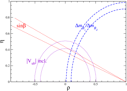
Figure 1: Constraints on the unitarity triangle. The bands show bounds at 1 $\sigma$ level.

As can be seen from Fig. 1, the results are consistent with unitarity with 2 $\sigma$ level. However, it is also true that there is still large room for new physics. Since the error is dominated by theory except for $\sin(2\phi_{1})=\sin(2\beta)$, it is crucial to reduce the theoretical errors in the lattice determination of weak matrix elements for heavy flavor physics for more stringent tests of the standard model and the physics beyond.

2 Heavy quark formalisms for heavy-light systems

2.1 Lattice NRQCD

Lattice NRQCD action is a discretized version of nonrelativistic effective action which is applicable for the heavy quark mass whose spatial momenta are smaller than the mass. The expansion parameter is the velocity of the heavy quark for quarkonia and $\Lambda/m$ for the heavy-light system where $\Lambda$ is the typical momenta for all the light degrees of freedom. Since it is a nonrenormalizable theory, one cannot take the continuum limit. Also the action and operator can be matched to full QCD only by perturbation theory. In order to control the discretization errors the action is often highly improved at the tree level. The dominant source of errors are perturbative errors.

2.2 Relativistic heavy quark (RHQ) formalism

The Femilab action [3] , AKT action [4] , and the relativistic heavy quark(called RHQ) action  [7] by RBC collaboration are the formalisms for heavy quark using improved Wilson fermion with suitably chosen improvement coefficients. The three formulations are essentially the same in the sense that they are Synamzik effective action applicable to quarks with small spatial momenta $|a\vec{p}|\ll 1$ where the coefficients are mass dependent. These actions smoothly interpolate the static quark and light quark. Therefore one can in principle take the continuum limit without encountering the breakdown of the theory. However, since the discretization and perturbative error of the physical observable depend on $am$, how the B meson physical observable approach to the continuum limit is nontrivial.

The discretization and perturbative errors are expected to be small by order estimation. Partial non perturbative (wavefunction) renormilzation using $Z_{V}^{nonpert}$ is useful. For higher accuracy both the discretization and perturbative error should be reduced. In order to reduce the perturbative error either two-loop calculation which is possible only by automated procedure [5] or nonperturbative renormalization. To reduce the discretization error further improvement by adding more terms is necessary. This is perused by FNAL, CP-PACS and RBC collaborations.

Lin and Christ  [6],[7] determined the coefficients of the RHQ action nonperturbatively in quenched QCD.

$$S = \sum_{n}\bar{\psi}_{n}[m_{0}+\gamma_{0}+\zeta\vec{\gamma}\cdot\vec{D}-\frac{1}{2}aD_{0}^{2}-\frac{\zeta}{2}\vec{D}^{2}-\sum_{i}\frac{i}{2}c_{E}a\sigma_{0i}F_{0i}-\sum_{i,j}\frac{i}{2}c_{B}a\sigma_{i}F_{ij}]\psi_{n}$$ (3)

They show that one can set $c_{E}=c_{B}=c_{P}$ by shifting $c_{E}$ and $c_{B}$ by field transformations

$$\psi\rightarrow(1-a^{2}[\gamma^{i},\gamma^{0}][D^{i},D^{0}]\xi_{E})\psi,$$ (4)

$$\psi\rightarrow(1-a^{2}[\gamma^{i},\gamma^{u}][D^{i},D^{j}]\xi_{B})\psi,$$ (5)

so that only three parameters$m_{0}$, $\zeta$ , $c_{P}$ should be tuned.

In order to determined the parameters nonperturbatively, they carry out the step scaling in three steps.

		finer lattice		coarser lattice
	L(fm)	size	$a^{-1}_{finer}$	sinze	$a^{-1}_{coarser}$(GeV)
Step 1	0.9	$24^{3}\times 48$	5.4 GeV	$16^{3}\times 32$	3.6
Step 2	1.3	$24^{3}\times 48$	3.6 GeV	$16^{3}\times 32$	2.4
Step 3	2.0	$24^{3}\times 48$	2.4 GeV	$16^{3}\times 32$	1.6

Table 1: lattice setup for step scaling

In step 1, one starts with a very fine lattice in small volume on which $am\ll 1$ is satisfied so that one can describe the heavy quark using Domain Wall fermion with controlled discretization error. One can then match the coefficients of the RHQ action on a coarser lattice for the same volume using one shell quantities: (1) the spin averaged 1S state mass for heavy-heavy and heavy-light system, (2) hyperfine splitting for heavy-heavy and heavy-light system, (3) the spin-orbit average and splitting for heavy-heavy system, and (4) the dispersion relation. In step 2, 3 and so on, they can repeat similar procedure to match RHQ on a lattice to RHQ on an even coarser lattice. They demonstrate that one can actually determine the parameters with reasonable accuracy and obtain improvements in charmonium spectrum compared to those with perturbatively determined parameters. This method is quite similar to nonperturbative HQET by Alpha collaboration which will be explained later. However, at the moment the step scaling function is defined not in the continuum limit but a fixed lattice spacing assuming discretization error is under control. It will be important to have theoretical understanding about how the systematic errors in the matching procedure can be controlled in this method.

2.3 Method with nonperturbative accuracy

Rome II group [8],[9] proposed a method to compute B physics observables with nonperturbative accuracy based on finite size scaling. Consider a physical observable ${\cal O}(E_{h},E_{l})$ which depends on two largely separated energy scales $E_{l}$ and $E_{h}(E_{l}\ll E_{h})$. They assume that the finite size effects has a mild dependence on high energy scale $E_{h}$. Then Finite size effects can be obtained from the ratio $\sigma_{\cal O}$ of the observable in two different volume $L$ and $2L$.

$$\sigma_{\cal O}(E_{l},E_{h},L)=\frac{{\cal O}(E_{l},E_{h},2L)}{{\cal O}(E_{l},E_{h},L)}$$ (6)

When $E_{l}\ll E_{h}$ the finite size correction can be expanded as

$$\sigma_{\cal O}(E_{l},E_{h},L)=\sigma_{\cal O}(E_{l},L)+\frac{\alpha^{(1)}(E_{l},L)}{E_{h}}+\frac{\alpha^{(2)}(E_{l},L)}{E_{h}^{2}}+\cdots.$$ (7)

In the case of heavy-light meson almost at rest, the high energy quantity $E_{h}$ is the heavy quark mass and the assumption that one can expand the physical observable ratio in $1/m$ is justified by HQET. Using the step scaling function $\sigma_{\cal O}$ one can obtain the physical observable in infinitely large volume as

$${\cal O}(E_{l},E_{h},L_{\infty})={\cal O}(E_{l},E_{h},L_{0})\sigma_{\cal O}(E_{l},E_{h},L_{0})\sigma_{\cal O}(E_{l},E_{h},2L_{0})\cdots$$ (8)

When the volume is $L_{0}$ small one can carry out lattice calculation with a cut off much larger than $E_{h}$ with reasonable numerical cost so that one can compute the physical observable directly at energy scale $E_{h}$ using the formalism of nonperturbatively O(a)-improved Wilson fermion. But as the volume gets larger through step scaling at some point $2^{k}L_{0}$ becomes too large one cannot afford very small lattice spacing so that direct computation becomes hopeless. However, one can always find a lower energy scale $E_{h}^{(k)}<E_{h}$ where direct calculation is possible. In this case one can use Eq. 7 to extrapolate $\sigma_{\cal O}(E_{l},E_{h}^{(k)},2^{k}L_{0})$ to $\sigma_{\cal O}(E_{l},E_{h},2^{k}L_{0})$. Since each step can be extrapolated in the continuum with nonperturbatively O(a)-improved Wilson fermion, the only systematic error in this procedure is the extrapolation in $1/E_{h}$. However, in order to take the continuum limit one has to know the parameter of constant physics so that one should know the master formula $\lambda_{QCD}$ scale and renormalization invariant quark mass as functions of the bare gauge coupling $g^{2}_{0}$ and the bare quark mass $m_{0}$. They find that in the case of the mass and the decay constant of the B meson mass one can practically control the extrapolation error at the level of few percent accuracy. The advantage is that this method is simple and promising. Probably, the Bag parameters, and form factors at zero recoil also fall into this category. Form factors for non zero recoil may be challenging.

The Alpha collaboration proposes HQET with nonperturbative accuracy  [10] for high precision computation in B physics. The action of HQET can be written with 1/m expansion as follows

$$L=L_{stat}+\sum_{\nu}^{n}L^{(\nu)},$$ (9)

$$L_{stat}=\bar{\psi}_{h}[D_{0}+\delta m]\psi_{h}, L^{(\nu)}=\sum_{i}\omega_{i}^{(\nu)}L_{i}^{(\nu)}$$ (10)

$L_{i}^{(\nu)}$ are the $1/m^{\nu}$ correction terms $\omega_{i}^{(\nu)}$ are their coefficients.

$$L_{1}^{(1)}=\bar{\psi}_{h}[-\frac{1}{2}\sigma\cdot B]\psi_{h}, L_{2}^{(1)}=\bar{\psi}_{h}[-\frac{1}{2}D^{2}]\psi_{h}.$$ (11)

Since the static theory has a continuum limit and is a renormalizable theory, if we expand the 1/m correction terms systematically to a fixed order $n$ as operator insertions, one can renormalize all the physical observable and take the continuum limit. In a very small volume where one can afford sufficiently fine lattice, the renormalization parameter can be determined nonperturbatively by carrying out QCD simulation for heavy quark with $O(a)$-improved Wilson and imposing the matching condition for a set of physical observables $\{\Phi_{k}(M,L_{0})\}$ as,

$$\Phi_{k}^{HQET}(M,L_{0})=\Phi_{k}^{QCD}(M,L_{0})+O(\frac{1}{M^{n+1}}),k=1,...,N_{n}$$ (12)

After matching QCD to HQET in small volume with lattice size $L_{0}$, one can then define the step scaling function $F_{k}$ as

$$\Phi_{k}^{HQET}(M,2L_{0})=F_{k}(\Phi_{k}^{HQET}(M,L_{0}))+O(\frac{1}{M^{n+1}}),k=1,...,N_{n}$$ (13)

By repeating this step, one can determine the matching conditions for $\omega_{i}^{(\nu)}$ for large and coarse lattices where one wants to carry out lattice simulation. During each step one can take the continuum limit so that the only systematic error is the truncation error in $1/M$. To control the truncation error $1/M\ll L_{0}$ is required which restricts the smallest possible $L_{0}$ as a function of $M$. This is in principle possible, but when one goes to higher order mixing with lower dimension operators through power divergences may give numerical difficulty, so that the calculation is technically more demanding.

In this conference Guazzini et al. [11] reported their proposal for further improvements. They combine the Rome II method and Alpha collaboration method. To be more precise, they basically follow the Rome II method, but hey also compute step scaling function $\sigma$ using nonperturbative HQET in the static limit. When they estimate the heavy quark mass dependence of the finite size correction, instead of extrapolating in 1/M, they make interpolation using the static result as an additional input.

3 Heavy-light decay constants

3.1 $f_{D_{s}}$, $f_{B_{s}}$ in quenched QCD

The determination of the heavy-light decay constants with nonperturbative accuracies is one of the most important progress.

Since the charm quark is of order 1 GeV, the decay constant $f_{D_{s}}$ in quenched approximation can be computed including nonperturbatively including the continuum limit with the present computer resources. Alpha collaboration [12]’s result for $a^{-1}=2-4$ GeV with $O(a)$-improved Wilson fermion is

$$f_{D_{s}}=252(9)\mbox{ MeV }.$$ (14)

The Rome II group [9] computed the heavy-light decay constants in quenched QCD using $O(a)$-improved Wilson fermion by step scaling method. The observable is the nonpertubatively improved heavy-light axial vector current in SF boundary for vanishing boundary gauge field with periodic spatial boundary condition for fermions. They prepared three different size for $L^{3}\times 2L$ volume with $L_{0}=0.4,L_{1}=0.8,L_{2}=1.6$ fm for step scaling. The lattice spacings and RGI heavy quark masses are $a=0.012-0.033fm$, $m^{RGI}=1.6-7.0$ GeV for $L=L_{0}$, $a=0.05-0.10fm$, $m^{RGI}=2.0-3.5$ for $L=L_{1}$ and $a=0.10-0.20fm$, $m^{RGI}=1.3-2.0$ for $L=L_{2}$ . Defining the finite volume corrections factors with the ratio of the decay constants for two different volumes as $\sigma(L_{0})\equiv\frac{f_{B_{s}}(2L_{0})}{f_{B_{s}}(L_{0})}$ and $\sigma(L_{1})\equiv\frac{f_{B_{s}}(L_{\infty})}{f_{B_{s}}(2L_{0})}$ , the decay constant in the infinite volume can be obtained as

$$f_{B_{s}}(L_{\infty})=f_{B_{s}}(L_{0})\sigma(L_{0})\sigma(L_{1}).$$ (15)

The result is

$$f_{B_{s}}(L_{0})=475(2)\mbox{MeV}, f_{D_{s}}(L_{0})=644(3)MeV$$ (16)

$$\sigma_{B_{s}}(L_{1})=0.417(3), \sigma_{D_{s}}(L_{1})=0.414(3)$$ (17)

$$\sigma_{B_{s}}(L_{1})=0.97(3), \sigma_{D_{s}}(L_{1})=0.90(2).$$ (18)

As it turned out, the heavy quark mass dependence of the step scaling function are indeed small, which justified the extrapolation. Combining these results

$$f_{B_{s}}=192(6)(4)\mbox{MeV}, f_{D_{s}}=240(5)(5)\mbox{MeV}.$$ (19)

Alpha collaboration [13] compute static heavy-light decay constant with lattice HQET which is matched to QCD with nonperturbative accuracy by Schrodinger functional method. They computed the renormalization group invariant matrix element $\Phi^{stat}_{RGI}$ which can be related to the decay constant by a matching factor $C_{PS}$ [14] as $\Phi^{stat}_{RGI}=f_{PS}\sqrt{m_{PS}}/C_{PS}$ and obtain

$$\Phi^{stat}_{RGI}=1.74(13)$$ (20)

Figure 2: Interpolation of static and relativistic results of heavy-light decay constant to obtain $f_{B_{s}}$. Figure taken from  [15].

Alpha collaboration [15] also computed the decay constants for the charm quark mass regime, i.e. $m_{Q}=1.7-2.6$ GeV, at four lattice spacings in the range $a=0.05-0.1$ fm using $O(a)$-improved Wilson fermion for both the heavy and the light quarks. They then interpolated the decay constants in the static limit and those for finite quark mass to obtain $f_{B_{s}}$. They found that both linear and quadratic interpolations lead to

$$f_{B_{s}}=206(10)\mbox{MeV}.$$ (21)

using $r_{0}=0.5$ fm for the scale input. as shown in Fig.2.

Guazzini et al. [11] reported a quenched study of $f_{B_{s}}$ with nonperturbative accuracy. Their approach uses the combination of the two methods. They compute the heavy-light decay constants in finite volumes both for the relativistic and static heavy quarks to the step scaling and “interpolate” the finite volume correction $f_{B_{s}}$ to using both the relativistic and the static. They computed the 2 point functions for static and relativistic heavy-light axial current with Schrodinger boundary conditions, where the boundary gauge fields $C=C^{\prime}=0$ and periodic boundary condition in the spatial directions $\theta=0$ for the light quark. The data for relativistic heavy-light current is obtained by the reanalysis of those by Rome II collaboration [9]. They chose $f_{hl}\sqrt{m_{hl}}$ for the physical observable rather than $f_{hl}$. Thus finite size corrections $\sigma_{1}$, $\sigma_{2}$ are defined by the ratio of $f_{hl}\sqrt{m_{hl}}$ for different volumes as

$$\sigma_{1}\equiv\frac{f_{hl}(2L_{0})\sqrt{m_{hl}}(2L_{0})}{f_{B_{s}}(L_{0})\sqrt{m_{hl}}(L_{0})}, \sigma_{2}\equiv\frac{f_{hl}(L_{\infty})\sqrt{m_{hl}}(L_{\infty})}{f_{B_{s}}(2L_{0})\sqrt{m_{hl}}(2L_{0})}$$ (22)

the infinite volume can be obtained as

$$f_{B_{s}}(L_{\infty})\sqrt{m_{B_{s}}(L_{\infty})}=f_{B_{s}}(L_{0})\sqrt{m_{B_{s}}(L_{0})}\sigma_{1}\sigma_{2}.$$ (23)

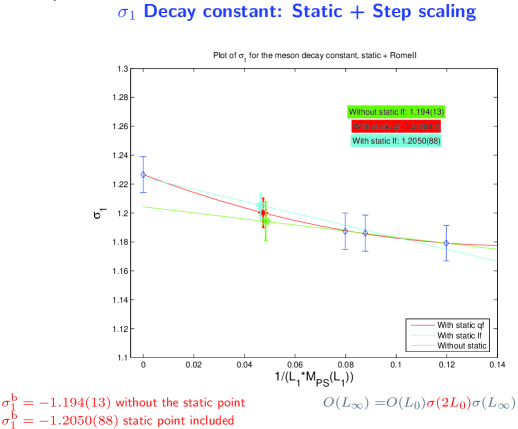
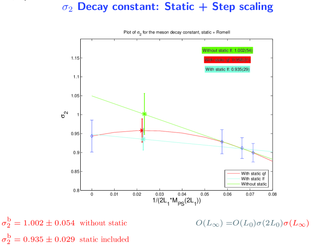
Figure 3: 1/M interpolation of the finite size corrections $\sigma_{1}$(top) and $\sigma_{2}$(bottom) for $f_{B_{s}}\sqrt{m_{B_{s}}}$. Figures from Guazzini’s talk.

As shown in Figs.3, the heavy quark mass dependences of the finite size corrections have much better control with the help of static results. Their preliminary quenched result is

$$f_{B_{s}}=186\pm 6\mbox{ MeV }$$ from Static + Rome II (24)

$$f_{B_{s}}=195\pm 11\mbox{ MeV }$$ from only Rome II (25)

which are consistent with previous results by Rome II and by Alpha collaborations.

There are also calculations of heavy-light decay constants with Ginsparg-Wilson fermions. The RBC collaboration [16] has carried out a quenched study of D meson using domain wall fermion and DBW2 gauge action. The quark mass ranges from $m_{q}=\frac{1}{4}m_{s}\sim\frac{5}{4}m_{s}$ and the lattice spacing is $a\sim 3$ GeV. Using the nonperturbative renormalization factor for the light-light axial vector current [17] and giving the mass correction as

$$Z_{A}^{hl}=Z_{A}^{ll,nonpert}\frac{Z_{q,DWF}(am_{heavy})}{Z_{q,DWF}(am_{light})},$$ (26)

their result is

$$f_{D_{s}} = 254(4)(12)\mbox{ MeV},$$ (27)

where the errors are statistical, and systematic errors. Chiu et al. [18], [19] also computed $f_{D}$ in quenched QCD using the optimal domain-wall fermion on a lattice with $a^{-1}=2.2$(GeV) for 30 quark masses $am_{q}=0.03-0.80$ using $f_{\pi}$ as scale input to find

$$f_{D_{s}} = 266(10)(18)\mbox{ MeV},$$ (28)

where the errors are statistical, and systematic errors.

3.2 $f_{D_{s}}$, $f_{B_{s}}$ in unquenched QCD

FNAL/MILC collaboration [20] reported preliminary results of $f_{B_{s}}$ for $n_{f}=2+1$ flavor QCD with MILC configuration. They use fermilab formalism for the heavy quark and improved staggered for the light quark. The lattice spacings are $a=0.090.12,0.15$ fm. The renormalization factor $Z_{A}$ is taken to be

$$Z^{Qq}_{A}=\rho_{A}^{Qq}\sqrt{Z_{V}^{QQ}Z_{V}^{qq}},$$ (29)

where $Z_{V}$’s are computed nonperturbatively and the remaining part $\rho_{A}$ is computed by one-loop perturbation theory. Their preliminary result is

$$f_{B_{s}}=253(7)(41)\mbox{ MeV}, f_{B_{s}}/f_{D_{s}}=0.99(2)(6),$$ (30)

where the errors are statistical error and systematic errors.

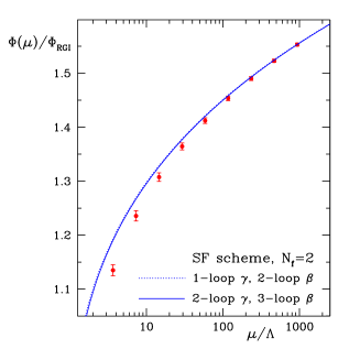
Figure 4: Step scaling of heavy-light axial current. Figure provided by J. Heitger.

Alpha collaboration [21] computed the renormalization factor for the static heavy-light axial vector current $Z_{A}^{stat}$ for $n_{f}=2$ unquenched QCD. Their preliminary result is shown in Fig. 4. Their preliminary result is

$$\Phi(L_{max})/\Phi_{RGI}=1.14(1),$$ (31)

where $L_{max}$ is the physical lattice size in which one wants to carry out the matrix element calculation. Using this result, once the large volume $n_{f}=2$ unquenched calculation $\beta=5.3$ for the regularization dependent renomalization factor $Z_{A}^{stat}(L_{max},g_{0})$ and the lattice bare matrix element $f_{B_{s}}^{stat}\sqrt{m_{B_{s}}})^{lat}(L_{max},g_{0})$ is done, one can obtain the static heavy-light decay constant as

$$f_{B_{s}}^{stat}\sqrt{m_{B_{s}}}=C_{PS}\frac{\Phi_{RGI}}{\Phi(L_{max})}Z_{A}^{stat}(L_{max},g_{0})(f_{B_{s}}^{stat}\sqrt{m_{B_{s}}})^{lat}(L_{max},g_{0}),$$ (32)

where $C_{PS}$ is perturbatively calculable conversion factor. The large volume $n_{f}=2$ simulation is now in progress for $\beta=5.3$.

3.3 Discussion on $f_{B_{s}}$, $f_{D_{s}}$ results

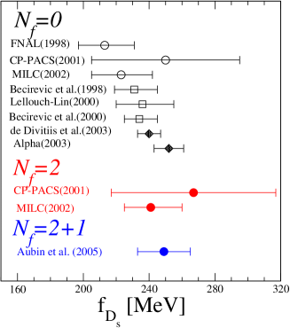
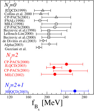
Figure 5: Decay constants $f_{D_{s}}$(left), $f_{B_{s}}$(right)

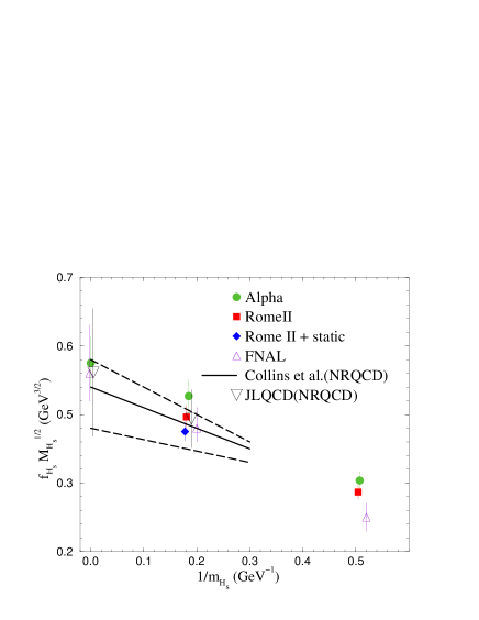
Figure 6: Comparison of 1/m dependence of $f\sqrt{m}$

Fig. 5 show the summary of decay constants $f_{B_{s}},f_{D_{s}}$ in quenched, $n_{f}=2$ unquenched, and $n_{f}=2+1$ unquenched lattice QCD. It should be noted that the quenched results are getting very precise owing to the recent developments with finite volume technique which allows us to compute nonperturbatively renormalized heavy-light decay constants in the continuum limit as discussed in the previous subsection. We take the average of the results from Rome II and Alpha collaboration as the best result in quenched approximation,

$$f_{B_{s}}^{n_{f}=0}=194(6)\mbox{ MeV}, f_{D_{s}}^{n_{f}=0}=245(6)\mbox{ MeV}, \left(\frac{f_{B_{s}}}{f_{D_{s}}}\right)^{n_{f}=0}=0.80(6),$$

In the unquenched case, the decay constants have larger errors from perturbative matching. I would quote the average of HPQCD/MILC and FNAL/MILC results for $f_{B}$ and FNAL/MILC results for $f_{D}$ as the best value. However, since the best result come from the same configuration, it would be worthwhile to study the heavy quark mass dependence and $n_{f}$ dependence based on the collection of results from various collaborations.

$n_{f}$	Group	heavy	light	$\frac{f_{B_{s}}}{f_{D_{s}}}$
0	MILC [23]	Wilson	Wilson	0.89(4)
	FNAL [24]	fermilab	clover	0.88(3)
	Lellouch-Lin [25]	clover	clover	0.82(5)
	Rome II [9]	clover	clover	0.80(4)
	Alpha [15]	clover	clover	0.81(6)
	RomeII+Alpha [11]	clover	clover	0.76(3)
2	MILC [26]	Wilson	Wilson	0.92(7)
2+1	FNAL/MILC [20]	fermilab	Imp Stag	0.99(2)(6)

Table 2: The decay constant ratio $f_{B_{s}}/f_{D_{s}}$.

Table 2 shows the ratio of $f_{B_{s}}/f_{D_{s}}$. Recent quenched calculations show smaller values of $\frac{f_{B_{s}}}{f_{D_{s}}}$. Fig. 6 shows the comparison of $1/M$ dependence of $f_{B_{s}}\sqrt{f_{m_{B_{s}}}}$ in quenched QCD near the static limit by Alpha, Rome II, FNAL, Collin’s et al. and JLQCD. It can be seen that the $1/M$ slope is consistently small independent of the action or collaborations. Parameterizing

$$f_{B_{s}}\sqrt{f_{m_{B_{s}}}}=(f_{B_{s}}\sqrt{f_{m_{B_{s}}}})^{stat}(1-\frac{c_{1}}{m_{B_{s}}}+\cdots),$$ (33)

both the Alpha collaboration and Collins et al give the slope of $c_{1}\sim 0.5-0.6$ GeV.

MILC results for $n_{f}=2$ suggest that sea quark effects may increase $\frac{f_{B_{s}}}{f_{D_{s}}}$ but not significantly due to the error. On the other hand, FNAL/MILC preliminary $n_{f}=2+1$ result presented in this conference suggests a significant increase in the $\frac{f_{B_{s}}}{f_{D_{s}}}$. However, one should bear in mind that the the systematic error is slightly different for B and D in fermilab formalism so that some consistency check is desired.

Group	heavy	$a^{-1}$ input	$\frac{f_{B_{s}}^{n_{f}=2}}{f_{B_{s}}^{n_{f}=0}}$	$\frac{f_{D_{s}}^{n_{f}=2}}{f_{D_{s}}^{n_{f}=0}}$	$\frac{f_{B_{s}}^{n_{f}=2+1}}{f_{B_{s}}^{n_{f}=0}}$
JLQCD  [27], [28]	NRQCD	$m_{\rho}$	1.13(5)	-	-
CP-PACS [29]	NRQCD	$\sigma$	1.10(5)	-	-
HPQCD [30]	NRQCD	$r_{0}$	-	-	$\sim$ 1.15
CP-PACS [31]	fermilab	$m_{\rho}$	1.14(5)	1.07(5)	-
MILC [23], [26]	Wilson	$f_{\pi}$	1.09(5)	1.08(5)	-

Table 3: $n_{f}$ dependence of $f_{B_{s}}$, $f_{D_{s}}$.

Table 3 is the collection of the $n_{f}$ dependence of the heavy-light decay constants $f_{B_{s}}$, $f_{D_{s}}$ using the same gauge and fermion action by the same group. It is seen that if the scale is set by the low energy inputs, turning on the sea quark effects from $n_{f}=0$ to $n_{f}=n+2$ to increases $f_{B_{s}}$ by 10-15% , while the increase is not significant for $f_{D_{s}}$. It is quite natural to expect the size of the sea quark effects for $f_{D_{s}}$ should be something between that for $f_{B_{s}}$ and $f_{K}$. And with the low energy inputs $f_{K}$ receives almost no sea quark effects by definition, the sea quark effects for $f_{B_{s}}$ should be larger than for $f_{D_{s}}$, which explains the above observations.

From Tables 3, 2, we also estimate the ratio of decay constants as

$$\frac{f_{B_{s}}^{n_{f}=2}}{f_{B_{s}}^{n_{f}=0}}=1.12(5), \frac{f_{D_{s}}^{n_{f}=2}}{f_{D_{s}}^{n_{f}=0}}=1.08(5),$$ (34)

$$\frac{f_{B_{s}}^{n_{f}=2+1}}{f_{B_{s}}^{n_{f}=0}}=1.15(5), \frac{f_{D_{s}}^{n_{f}=2+1}}{f_{D_{s}}^{n_{f}=0}}=1.10(5).$$ (35)

This can give an educated guess for $n_{f}=2$ decay constants. However, there are several uncertainties in this argument. First, the up/down sea quark mass for the unquenched configuration other than MILC may not small enough to fully reproduce the sea quark effects. Also when one uses low energy inputs the scale suffer from the chiral extrapolation uncertainty. Although Sommer scale $r_{0}$ is relatively stable, but the phenomenological value of $r_{0}=0.5$ fm also suffer from uncertainty which is typically 10%. Our educated guess for $n_{f}=2$ results are

$$f_{B_{s}}^{n_{f}=2}=217(12)(22)\mbox{ MeV}, f_{D_{s}}^{n_{f}=2}=265(14)(27)\mbox{ MeV},$$ (36)

$$f_{B_{s}}^{n_{f}=2+1}=223(17)(22)\mbox{ MeV}, f_{D_{s}}^{n_{f}=2}=270(18)(27)\mbox{ MeV},$$ (37)

where the second error is added to take account the scale uncertainties of order 10%. On the other hand the average based on the actual data of decay constant in $n_{f}=2+1$ QCD by FNAL/MILC and FNAL/MILC collaborations are

$$f_{B_{s}}^{n_{f}=2+1}=260(30)\mbox{ MeV}, f_{D_{s}}^{n_{f}=2+1}=249(16)\mbox{ MeV},$$ (38)

which is marginally consistent with our estimate within errors. Combining my educated guess and HPQCD/MILC, FNAL/MILC results my ’world average’ would be

$$f_{B_{s}}^{n_{f}=2+1}=240(30)\mbox{ MeV}, f_{D_{s}}^{n_{f}=2+1}=260(20)\mbox{ MeV}.$$ (39)

3.4 chiral extrapolation

In order to obtain $f_{B_{d}}$ and $f_{D_{d}}$ one has to take the chiral extrapolation. This offers another important issue for precise determination of the decay constant in addition to the problems discussed for $f_{B_{s}}$ and $f_{D_{d}}$. The correct answer can only be obtained with unquenched calculation. The chiral perturbation theory tells us that the chiral logarithmic corrections to the SU(3) breaking ratio of the decay constants is  [33]

$${f_{B_{s}}\sqrt{m_{B_{s}}}\over f_{B_{d}}\sqrt{m_{B_{d}}}}=1+{1+3{\hat{g}}^{2}\over 4(4\pi f)^{2}}\left(3m_{\pi}^{2}\log{m_{\pi}^{2}\over\Lambda}\right.\left.-2m_{K}^{2}\log{m_{K}^{2}\over\Lambda}-m_{\eta}^{2}\log{m_{\eta}^{2}\over\Lambda}\right)+\cdots.$$ (40)

FNAL/MILC collaboration [20] reported preliminary results from $n_{f}=2+1$ heavy-light decay constants in the previous subsection. With the staggered quark the pseudoscalar mesons for each flavor quantum number ($I$) has 16 tastes labeled by $\xi=P,A,T,V,I$. Their masses are splitted as

$$m^{2}_{I}=(m_{a}+m_{b})\mu+a^{2}\Delta_{\xi}, \xi=P,A,T,V,I$$ (41)

The staggered chiral perturbation theory suggests that the quark mass dependence of the heavy-light decay constant $\Phi_{H_{q}}\equiv f_{H_{q}}\sqrt{m_{H_{q}}}$ is

$$\Phi_{H_{q}}=\Phi_{H}[1+\frac{\delta f_{H_{q}}}{16\pi^{2}f^{2}}+\mbox{ analytic terms }],$$ (42)

where the explicit form of $\delta f_{H_{q}}$, which is the analog of the chiral log in the continuum chiral perturbation theory, can be obtain from staggered chiral perturbation theory [35]. Due to the taste symmetry breaking of $O(a^{2})$ terms they have many parameters for $a^{2}$ effects which have to be fitted from the lattice spacing dependence of the lattice data. Some parameters can be obtained from the pion system but other parameters have to be fitted from the data of the heavy-light decay constants themselves. Their preliminary results are

$$(f_{D_{s}}/f_{D_{d}})^{n_{f}=2+1}=1.21(1)(4). (f_{B_{s}}/f_{B_{d}})^{n_{f}=2+1}=1.27(2)(6),$$ (43)

where the errors are statistical and systematic errors.

Gadiyak and Loktik [32] made a $n_{f}=2$ unquenched study of SU(3) breaking effect using domain wall fermion and DBW2 gauge action. The quark mass ranges from $m_{\pi}=490,610,700$ MeV and the lattice spacing is $a\sim 1.69(5)$ GeV. They found that

$$(f_{B_{s}}/f_{B_{d}})^{n_{f}=2}=1.29(4)(4)(2).$$ (44)

Group	heavy	light	$n_{f}$	$f_{B_{s}}/f_{B_{d}}$	visible chiral log
CP-PACSS [29]	NQCD	clover	2	1.18(2)(2)	NO
CP-PACS  [31]	fermilab	clover	2	1.20(3)(3)(${}^{+4}_{-0}$)	NO
MILC [26]	fermilab	Wilson	2	1.16(1)(2)(2)(${}^{+4}_{-0}$)	NO
JLQCD [28]	NRQCD	clover	2	1.13(3)(${}^{+13}_{-0}$)	NO
Gadiyak and Loktik [32]	static	DW	2	1.29(4)(6)	NO
HPQCD/MILC [30]	NRQCD	Imp Stag	2+1	1.20(3)(1)	YES
FNAL/MILCC [20]	fermilab	Imp Stag	2+1	1.27(2)(6)	YES

Table 4: SU(3) breaking ratio $f_{B_{s}}/f_{B_{d}}$

Group	heavy	light	$n_{f}$	$f_{D_{s}}/f_{D_{d}}$	visible chiral log
CP-PACSS  [31]	fermilab	clover	2	1.18(4)(3)(${}^{+4}_{-0}$)	NO
MILC [26]	fermilab	Wilson	2	1.14(1)(${}^{+2}_{-3}$) (2)(${}^{+5}_{-0}$)	NO
FNAL/MILC [20]	fermilab	Imp Stag	2+1	1.21(1)(4)	YES

Table 5: SU(3) breaking ratio $f_{D_{s}}/f_{D_{d}}$

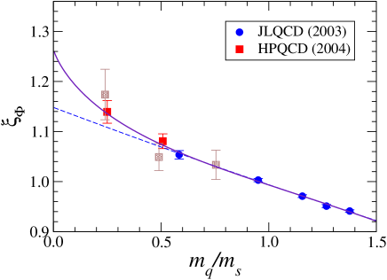
Figure 7: light quark mass dependence of $\Phi_{B_{s}}/\Phi_{B_{q}}$, where $\Phi=\sqrt{m_{B}}f_{B}$ .

Tables 4,5 show the collections of the unquenched results of $f_{D_{s}}/f_{D_{d}}$ and $f_{B_{s}}/f_{B_{d}}$. Except for FNAL/MILC and HPQCD/MILC, they do not observe the chiral log. This is natural because other results use much heavier light quarks. Fig.7 show the comparison of the light quark mass dependence of $f_{B_{s}}\sqrt{m_{B_{s}}}/f_{B_{d}}\sqrt{m_{B_{d}}}$ from JLQCD and HPQCD. They show consistent behavior for larger light quark mass. It seems that the JLQCD result may be missing the possible onset of chiral log which is found by HPQCD data. However, the results with MILC configuration are obtained through the staggered chiral perturbation theory, which requires quite complicated analysis with many parameters. Independent calculations with other formalisms are needed.

4 Bag parameters

The bag parameters that parameterizes the $B_{q}^{0}-\overline{B^{0}_{q}}$ mixing amplitude are defined by

$$\langle\bar{B}^{0}_{q}|\bar{b}^{i}\gamma_{\mu}(1-\gamma_{5})q^{i}\,\bar{b}^{j}\gamma_{\mu}(1-\gamma_{5})q^{j}|B^{0}_{q}\rangle ={8\over 3}\,m_{B_{q}}^{2}f_{B_{q}}^{2}B_{B_{q}} \ (\mbox{ where }q=d,s),$$ (45)

$$\langle\bar{B}^{0}_{s}|\bar{b}^{i}(1-\gamma_{5})q^{i}\,\bar{b}^{j}(1-\gamma_{5})s^{j}|B^{0}_{s}\rangle =-{5\over 3}\,m_{B_{s}}^{2}f_{B_{s}}^{2}\frac{B_{S}}{R^{2}} \ (\mbox{ where }R\equiv\frac{(\bar{m_{b}}+\bar{m_{s}})}{m_{B_{s}}}),$$ (46)

$$\langle\bar{B}^{0}_{s}|\bar{b}^{i}(1-\gamma_{5})q^{j}\,\bar{b}^{j}(1-\gamma_{5})q^{i}|B^{0}_{q}\rangle ={1\over 3}\,m_{B_{q}}^{2}f_{B_{q}}^{2}\frac{\tilde{B}_{S}}{R^{2}}$$ . (47)

HPQCD [36] computed the bag parameters for $B_{s}$ mixing calculation with improved $n_{f}=2+1$ dynamical staggered quark. The simulation was carried out using NRQCD action for heavy quark and AsqTad action for light quark on a $20^{3}\times 64$ lattice with $a^{-1}\sim 1.6$ GeV with the valence light quark mass at$m_{s}$ and the ud sea quark mass at $0.25m_{s}$, $0.5m_{s}$. They computed the matrix elements for three types of $\Delta B=2$ four fermion operators which correspond to $f_{B_{s}}^{2}B_{B_{s}}$, $f_{B_{s}}^{2}\frac{B_{S}}{R^{2}}$ and $f_{B_{s}}^{2}\frac{\tilde{B}_{S}}{R^{2}}$.

Defining $\Delta B=2$ four-fermion operators as

$$OL \equiv [\bar{b}^{i}q^{i}]_{V-A}[\bar{b}^{j}q^{j}]_{V-A},$$ (48)

$$OS \equiv [\bar{b}^{i}q^{i}]_{S-P}[\bar{b}^{j}q^{j}]_{S-P},$$ (49)

$$Q3 \equiv [\bar{b}^{i}q^{J}]_{S-P}[\bar{b}^{j}q^{I}I_{S-P},$$ (50)

$$OLj1 \equiv \frac{1}{2M}{[\vec{\nabla}\bar{b}^{i}\vec{\gamma}q^{i}]_{V-A}[\bar{b}^{j}q^{j}]_{V-A}+[\bar{b}^{i}q^{i}]_{V-A}[\vec{\nabla}\bar{b}^{j}\vec{\gamma}q^{j}]_{V-A}},$$ (51)

$$OSj1 \equiv \frac{1}{2M}{[\vec{\nabla}\bar{b}^{i}\vec{\gamma}q^{i}]_{S-P}[\bar{b}^{j}q^{j}]_{S-P}+[\bar{b}^{i}q^{i}]_{S-P}[\vec{\nabla}\bar{b}^{j}\vec{\gamma}q^{j}]_{S-P}},$$ (52)

$$Q3j1 \equiv \frac{1}{2M}{[\vec{\nabla}\bar{b}^{i}\vec{\gamma}q^{j}]_{S-P}[\bar{b}^{j}q^{i}]_{S-P}+[\bar{b}^{i}q^{j}]_{S-P}[\vec{\nabla}\bar{b}^{j}\vec{\gamma}q^{i}]_{S-P}},$$ (53)

where $i,j$ are color indices. The former three are operators in the leading order in $1/M$ and the latter three operators are $O(1/M)$ operators. The lattice operator is matched to that in the continuum using one-loop perturbation theory as

$$\frac{1}{2m_{B_{s}}}\langle OL\rangle^{\bar{MS}} = +[1+\alpha\rho_{LL}]\langle OL\rangle_{eff}+\alpha\rho_{LS}\langle OS\rangle_{eff}$$ (55)

$$+[\langle OL\rangle_{eff}-\alpha(\zeta_{10}^{LL}\langle OL\rangle_{eff}+\zeta_{10}^{LS}\langle OS\rangle_{eff})],$$

$$\frac{1}{2m_{B_{s}}}\langle OS\rangle^{\bar{MS}} = +[1+\alpha\rho_{SS}]\langle OS\rangle_{eff}+\alpha\rho_{SL}\langle OL\rangle_{eff}$$ (57)

$$+[\langle OSj1\rangle_{eff}-\alpha(\zeta_{10}^{SL}\langle OL\rangle_{eff}+\zeta_{10}^{SS}\langle OS\rangle_{eff})],$$

$$\frac{1}{2m_{B_{s}}}\langle Q3\rangle^{\bar{MS}} = +[1+\alpha\rho_{33}\langle Q3\rangle_{eff}+\alpha\rho_{3L}\langle OL\rangle_{eff}$$ (59)

$$+[\langle Q3j1\rangle_{eff}-\alpha(\zeta_{10}^{3L}\langle OL\rangle_{eff}+\zeta_{10}^{33}\langle Q3\rangle_{eff})].$$

It should be noted that in this work dimension 7 operators are included for the first time in NRQCD. Previous work by Hiroshima group [38] and JLQCD [39, 28] include only dimension 6 operators.

They find that the sea quark mass is only a few percent and quote the result for $m_{sea}=0.25m_{s}$ as their best value.

$$f_{B_{s}}\sqrt{\hat{B}_{B_{s}}}=0.281(20)\mbox{GeV}, f_{B_{s}}\sqrt{B_{B_{s}}}=0.227(16)\mbox{GeV},$$ (60)

$$f_{B_{s}}\sqrt{\frac{B_{S}}{R}}=0.295(21)\mbox{GeV}, f_{B_{s}}\sqrt{\frac{\tilde{B}_{S}}{R}}=0.305(21)\mbox{GeV}$$ (61)

The key points of HPQCD’s result is that the direct calculation of $f_{B_{s}}^{2}B_{B_{s}}$ gives better accuracy than computing $f_{B_{s}}$ and $B_{B_{s}}$ separately. The bag parameter has a smaller central value than that of JLQCD ($n_{f}=2$) after including $1/M$ correction (dime=7 operator), which is not included in JLQCD’s calculation. On the other hand, $f_{B_{s}}$ has a larger central value than JLQCD so that $f_{B_{s}}^{2}B_{B_{s}}$ is consistent Table 6.

$f_{B_{s}}\sqrt{\hat{B}_{B_{s}}}$ is related to the mass difference in $B_{s}-\bar{B}_{s}$ mixing as

$$\Delta m_{B_{s}} = \frac{G_{F}^{2}}{\eta}_{B}m_{B_{s}}f_{B_{s}}^{2}\hat{B}_{B_{s}}m_{W}^{2}S_{0}(m_{t}^{2}/m_{W}^{2})|V_{ts}V_{tb}|,$$ (62)

where $\eta$ is perturbatively calculable factor and $S_{0}(m_{t}^{2}/m_{W}^{2})$ is the Inami-Lim function. CDF [1] recently measured the mass difference as

$$\Delta m_{B_{s}}=18.3(^{+4}_{-2})\mbox{ps}^{-1}$$ (63)

Combining this with recent $|V_{cb}|$ value and CKM unitarity relation, the above equation requires $f_{B_{s}}\sqrt{\hat{B}_{B_{s}}}=0.245(20)$ (GeV).

Using heavy quark expansion the width difference of $B_{s}-\bar{B}_{s}$ mixing can be obtained at NLO as

$$\left(\frac{\Delta\Gamma}{\Gamma}\right)_{B_{s}} = \frac{16\pi^{2}B(B_{s}\rightarrow Xe\nu)}{g(m_{c}^{2}/m_{b}^{2})\tilde{\eta}_{QCD}}\frac{f_{B_{s}}^{2}m_{B_{s}}}{m_{b}^{3}}|V_{cs}|^{2}$$ (64)

$$\times\left(G(z)\frac{8}{3}B_{B_{s}}(m_{b})+G_{S}(z)\frac{5}{3}\frac{B_{S_{s}}(m_{b})}{R(m_{b})^{2}}+\sqrt{1-4mc^{2}/m_{b}^{2}}\delta_{1/m}\right),$$

where $g(z)=1-8z+8z^{3}-z^{4}-12z^{2}\ln z$ and $\tilde{\eta}_{QCD}$ is the short distance QCD correction. $G(z)$ and $G_{S}(z)$ are NLO QCD corrections which appear in OPE. $\delta_{1/m}$ is the NLO contribution in $1/m_{b}$ expansion. Using HPQCD results they predict

$$\left(\frac{\Delta\Gamma}{\Gamma}\right)_{B_{s}}=0.16(3)(2),$$ (65)

where the second errors comes from the uncertainty in the correction term $\sqrt{1-4mc^{2}/m_{b}^{2}}\delta_{1/m}$.

$n_{f}$	group	heavy	$B_{B_{s}}(m_{b})$	$B_{B_{s}}(m_{b})$	$B_{B_{s}}(m_{b})$
0	Becirevic. et al. [37]	HQET	0.87(5)	0.84(4)	0.91(8)
0	JLQCD [39]	NRQCD	0.84(5)	0.85(5)	-
2	JLQCD [28]	NRQCD	0.85(6)	-	-
2+1	HPQCD [36]	NRQCD	0.76(11)	0.84(12)	0.90(13)

Table 6: The bag parameters and $B_{B_{s}}^{\overline{\rm MS}}(m_{b})$

$n_{f}$	group	heavy	$B_{B_{d}}(m_{b})$
0	UKQCD	HQET	0.87(5)
0	Becirevic. et al. [37]	HQET	0.87(6)
0	JLQCD [39]	NRQCD	0.84(6)
2	JLQCD [28]	NRQCD	0.84(6)

Table 7: The bag parameters and $B_{B_{d}}^{\overline{\rm MS}}(m_{b})$

Table 7 gives the summary of $B_{B_{d}}$ from various collaborations. It should be noted that HPQCD’s result with $1/m$ correction in the operator gives lower values. Further understanding of $1/m$ dependence is required. On the other hand, the light quark mass dependence seems small from the data. In fact, chiral perturbation theory [33] suggests that the light quark mass dependence is

$${\hat{B}_{B_{s}}\over\hat{B}_{B_{d}}}=1+\frac{1-3{\hat{g}}^{2}}{(4\pi f)^{2}}m_{\pi}^{2}\log m_{\pi}^{2}+\cdots.\;,$$ (66)

Since $g\sim 0.6$, The coefficient of the chiral log is very small, which agrees with the lattice results.

5 $B\rightarrow\pi l\nu$ form factors

The matrix element $\langle\pi(k_{\pi})|\bar{q}\gamma_{\mu}b|B(p_{B})\rangle$ for the heavy-to-light semi-leptonic decay $B\rightarrow\pi l\nu$ is often parameterized as

$$\langle\pi(k_{\pi})|\bar{q}\gamma^{\mu}b|B(p_{B})\rangle=f^{+}(q^{2})\left[(p_{B}+k_{\pi})^{\mu}-\frac{m_{B}^{2}-m_{\pi}^{2}}{q^{2}}q^{\mu}\right]+f^{0}(q^{2})\frac{m_{B}^{2}-m_{\pi}^{2}}{q^{2}}q^{\mu},$$ (67)

with $p_{B}$ and $k_{\pi}$ the momenta and $q=p_{B}-k_{\pi}$. The differential decay rate of the semileptonic $B^{0}\rightarrow\pi^{-}l^{+}\nu_{l}$ decay is

$$\frac{1}{|V_{ub}|^{2}}\frac{d\Gamma}{dq^{2}}=\frac{G_{F}^{2}}{24\pi^{3}}|\vec{k}_{\pi}|^{3}|f^{+}(q^{2})|^{2}.$$ (68)

from which one can extract the CKM element $|V_{ub}|$.

HPQCD collaboration [40] has made a new study of $B\rightarrow\pi l\nu$ form factors using 2+1 flavor MILC configuration with $a^{-1}=1.6,2.3$ GeV. They used NQCD action for the heavy quark and improved staggered fermion for the light quark. The light quark mass ranges $m_{q}/m_{s}=0.125-0.5$ on the coarse lattice and $m_{q}/m_{s}=0.2-0.4$ on the fine lattice. The heavy-light vector current is renormalized with 1-loop matching through $O(\alpha/M)$ and $O(\alpha a)$. The chiral extrapolation is carried out using staggered chiral perturbation theory. In order to make the analysis convenient they parameterize the matrix element as

$$\langle\pi(k_{\pi})|V^{\mu}|B(p_{B})\rangle = \sqrt{2m_{B}}[v^{\mu}f_{\parallel}+k^{\mu}_{\perp}f_{\perp}],$$ (69)

with

$$v^{\mu}=\frac{p_{B}^{\mu}}{m_{B}}, k^{\mu}_{\perp}=k_{\pi}^{\mu}-(k_{\pi}\cdot v)v^{\mu}.$$ (70)

In order to interpolate in $q^{2}$, they used several different pole model fit functions. The first one is BK parameterization with three parameters with $\tilde{q}^{2}\equiv q^{2}/m_{B^{*}}$ ,

$$f^{+}(q^{2})=\frac{f(0)}{(1-\tilde{q}^{2})(1-\alpha\tilde{q}^{2})}, f^{0}(q^{2})=\frac{f(0)}{(1-\tilde{q}^{2}/\beta)}.$$ (71)

The second one is BZ parameterization with four parameters

$$f^{+}(q^{2})=\frac{f(0)}{(1-\tilde{q}^{2})}+\frac{r\tilde{q}^{2}}{(1-\tilde{q}^{2})(1-\alpha\tilde{q}^{2})},$$ (72)

The third one is RH parameterization with four parameters

$$f^{+}(q^{2})=\frac{f(0)(1-\delta\cdot\tilde{q}^{2})}{(1-\tilde{q}^{2})(1-\tilde{q}^{2}/\gamma)}.$$ (73)

For all three cases the parameterization is the same for $f^{0}$, First, the momentum dependent form factor data is interpolated to fixed $E_{\pi}$’s using these parameterization. Second, the chiral limit is taken for each fixed $E_{\pi}$ using staggered chiral perturbation theory [35]. It turns The results with different parameterizations are very well consistent with each other. Choosing BZ parameterization for the best result, they obtain

$$\frac{1}{|V_{ub}|^{2}}\int_{16GeV^{2}}^{q^{2}_{m}ax}\frac{d\Gamma}{dq^{2}}=1.46(23)(27)\mbox{ psec${}^{-1}$}$$

Using the experimental data from HFAG [42] $Br(q^{2}>16GeV^{2})=0.40(4)(4)\times 10^{-4}$, it leads to

$$|V_{ub}|=4.22(30)(51)\times 10^{-3},$$ (74)

which should be compared with FNAL/MILC results [41],

$$|V_{ub}|=3.76(25)(65)\times 10^{-3}$$ (75)

(See Fig. 8). Table 8 shows the partial branching fraction for $q^{2}>16GeV^{2}$ for various lattice calculations. So far within large errors, all the results are consistent. The average of $n_{f}=2+1$ results seems somewhat smaller than that of $n_{f}=0$ but not significantly.

$n_{f}$	Group	heavy	$\frac{\Gamma(q^{2}>16GeV^{2})}{|V_{ub}|^{2}}$ ps-1
0	UKQCD [44]	clover	2.30(${}^{+77}_{-51}$)(51)
0	APE [45]	clover	1.80(${}^{+89}_{-71}$)(47)
0	FNAL [46]	fermilab	1.91(${}^{+46}_{-13}$)(31)
0	JLQCD [47]	NRQCD	1.71(66)(46)
2+1	HPQCD/MILC [40]	NRQCD	1.46(23)(27)
2+1	FNAL/MILC [41]	fermilab	1.83(50)

Table 8: Values for partial branching fraction $\frac{\Gamma(q^{2}>16GeV^{2})}{|V_{ub}|^{2}}$ ps^-1 for various lattice calculations.

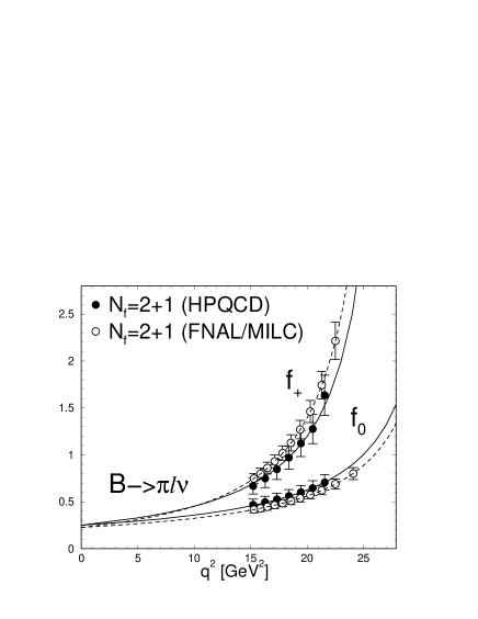
Figure 8: $B\rightarrow\pi l\nu$ form factors in $n_{f}=2+1$ QCD.

6 $m_{b}$

Alpha collaboration made a quenched study of $1/M$ corrections to HQET, which is an update of last years work. Matching of QCD and HQET at small volume, step scaling in HQET towards larger volume and computation of $m_{B_{s}}$ in large volume and finally convert to $m_{b}$. Last year they quoted that value

$$m_{b}^{\overline{MS}}=m_{b}^{stat}+m_{b}^{(1)},$$ (76)

$$m_{b}^{stat}=4.350(64)\mbox{GeV}, m_{b}^{(1)}=0.049(29)\mbox{GeV}$$ (77)

Guazzini et al. [11] computed the bottom quark mass using similar finite size scaling as $f_{B}$. Their preliminary results are

$$m_{b}^{RGI}=6.96(11) \mbox{(only Rome II)},$$ GeV (78)

$$m_{b}^{RGI}=6.89(11) \mbox{(Static + Rome II)}.$$ GeV (79)

Kronfeld and Simone [49] made a quenched study of HQET parameter $\bar{\Lambda}$, $\lambda_{1}$, and $m_{b}$. The idea is that HQET relation the heavy-light meson mass can be expressed as

$$M(m)=m+\bar{\Lambda}+\frac{\lambda_{1}}{2m}-d_{J}\frac{\lambda_{2}}{2m}+O(1/m^{2}).$$ (80)

Fitting the mass dependence of the heavy-light meson from lattice calculation one can extract $\bar{\Lambda}$, $\lambda_{1}$, and $m_{b}$ in lattice scheme. Using perturbation theory one can then convert HQET parameters to another short distance scheme free from renormalon ambiguities. Application of this method by to $n_{f}=2+1$ unquenched QCD by Fermilab collaboration is reported in this conference [50].

$n_{f}$	Renormalization	Group	$\bar{m}_{b}(\bar{m}_{b})$ (GeV)
$m_{B_{s}}$ and HQET
0	NNLO	Martinelli, Sacrahjda [51]	4.38(5)(10)
	Non pert.	Della Morte et al. [52]	4.350(64)
2	NNNLO	Renzo et al. [53]	4.21(3)(5)(4)
	NNLO	McNeile et al. [54]	4.25(2)(10)
$\Upsilon$ and NRQCD
2+1	NLO	Gray et al. [55]	4.4(3)
	NLO	Nobes, Trottier [56]	4.7(4)

Table 9: $\bar{m}_{b}(\bar{m}_{b})$

Recently HQET parameters are extracted by the global fit of the various moments for inclusive B decays such as $\langle E_{l}^{n}\rangle$, $\langle m_{X}^{2n}\rangle$ in $B\rightarrow X_{c}l\nu$ or $\langle E_{\gamma}^{n}\rangle$, in $B\rightarrow X_{s}\gamma$ . The result [57] is

$$m_{b}^{\overline{MS}}=4.20(2)(5)\mbox{ GeV},$$

where the first and the second errors are the experimental and theoretical errors. These determination is used to improve the accuracy of $|V_{cb}|$ and $|V_{ub}|$ determinations from inclusive semileptonic decays. A better determination of HQET parameters would provide further improvement in $|V_{cb}|$ and $|V_{ub}|$ determinations, which will be possible near future. Summary of recent results are given in Table 9.

7 New methods

7.1 Dispersive bounds for form factors

The momentum range of $B\rightarrow\pi l\nu$ form factors computed from Lattice QCD is limited by the small recoil or large $q^{2}$ region. This leads to a big disadvantage because most of the experimental data lies in large recoil region. While one can extrapolate in $q^{2}$ with a fit ansatz, this will always introduce some model dependence. Dispersive bounds is one possible way to constrain the $q^{2}$ dependence in model independent fashion using unitarity.

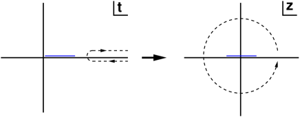
Figure 9: A map from $t$ plane to $z$ plane

Consider the imaginary part of the vacuum polarization amplitude for the current $V(x)=\bar{u}\gamma_{\mu}b(x)$ and a map as in Fig. 9

$$\!\!\Pi^{\mu\nu}(q) \equiv i\int d^{4}x\,e^{iq\cdot x}\langle 0|T\left\{V^{\mu}(x)V^{\nu\dagger}(0)\right\}|0\rangle$$ (81)

$$= (q^{\mu}q^{\nu}-g^{\mu\nu}q^{2})\Pi_{1}(q^{2})+q^{\mu}q^{\nu}\Pi_{0}(q^{2})\,,$$

$$z(t,t_{0}) = \frac{\sqrt{t_{+}-t}-\sqrt{t_{+}-t_{0}}}{\sqrt{t_{+}-t}+\sqrt{t_{+}-t_{0}}},\ (\mbox{ with }t_{\pm}=(m_{B}\pm m_{\pi})^{2}),$$ (82)

Then, from dispersion relations one obtains

$$\chi_{F_{+}}(Q^{2}) = {1\over 2}{\partial^{2}\over\partial(q^{2})^{2}}\left[q^{2}\Pi_{1}\right]={1\over\pi}\int_{0}^{\infty}\!dt\,{t{\rm Im}\Pi_{1}(t)\over(t+Q^{2})^{3}}\,,$$

$$\chi_{F_{0}}(Q^{2}) = {\partial\over\partial q^{2}}\left[q^{2}\Pi_{0}\right]={1\over\pi}\int_{0}^{\infty}\!dt\,{t{\rm Im}\Pi_{0}(t)\over(t+Q^{2})^{2}}\,.$$ (83)

with $Q^{2}=-q^{2}$ and $\eta$ an isospin factor, while $\chi$ ’s can be computed using OPE and perturbative QCD. Unitarity tells us that this is equal to the sum over all the hadronic states. and dropping all the excited states and leaving only the B $\pi$ state gives an exact bound.

$${\eta\over 48\pi}{[(t-t_{+})(t-t_{-})]^{3/2}\over t^{3}}|F_{+}(t)|^{2} \leq {\rm Im}\Pi_{1}(t)\,,$$

$${\eta t_{+}t_{-}\over 16\pi}{[(t-t_{+})(t-t_{-})]^{1/2}\over t^{3}}|F_{0}(t)|^{2} \leq {\rm Im}\Pi_{0}(t)\,,$$ (84)

shows that an upper bound on the norm can be established by choosing [recall that $|z|=1$ along the integration contour in (83)]

$$\phi_{+}(t,t_{0}) = \sqrt{\eta\over 48\pi}{t_{+}-t\over(t_{+}-t_{0})^{1/4}}\left(z(t,0)\over-t\right)\left(z(t,-Q^{2})\over-Q^{2}-t\right)^{3/2}\left(z(t,t_{0})\over t_{0}-t\right)^{-1/2}\left(z(t,t_{-})\over t_{-}-t\right)^{-3/4}\,,$$

$$\phi_{0}(t,t_{0}) = \sqrt{\eta t_{+}t_{-}\over 16\pi}{\sqrt{t_{+}-t}\over(t_{+}-t_{0})^{1/4}}\left(z(t,0)\over-t\right)\left(z(t,-Q^{2})\over-Q^{2}-t\right)\left(z(t,t_{0})\over t_{0}-t\right)^{-1/2}\left(z(t,t_{-})\over t_{-}-t\right)^{-1/4}\,.$$ (85)

Combining Eqs. 83, 84,  85 and making change of variables in the integration from $t$ to $z$. We obtain

$$\langle\phi f_{0}|\phi f_{0}\rangle<\chi_{0}, \langle P\phi f_{+}|P\phi f_{+}\rangle<\chi_{+},$$ (86)

where J is a quantity which can be obtained using OPE and perturbative QCD. The inner product $\langle g|h\rangle$ for arbitrary functions $g(z)$ and$h(z)$ is defined by the integral along the unit circle in $z$ plane as

$$\langle g|h\rangle\equiv\int\frac{dz}{2\pi i}(g(z))^{\ast}.$$ (87)

$P(z)=z(t,m_{B}^{*})$ is multiplied to $f_{+}$ in order to remove $B^{*}$ pole inside the unit circle. Cauchy’s theorem tells that if we know additional integrated quantity $\langle g_{i}|P\phi_{+}f_{+}\rangle$ with a set of known functions $\{g_{i}(z),i=1,...,N\}$ one can make the bound stronger as

$$\det\left(\begin{array}[]{cccc}\chi&\langle P\phi_{+}f_{+}|g_{1}\rangle&\ldots&\langle P\phi_{+}f_{+}|g_{N}\rangle\\ \langle g_{1}|P\phi f_{+}\rangle&\langle g_{1}|g_{1}\rangle&\ldots&\langle g_{1}|g_{N}\rangle\\ \vdots&\vdots&\ddots&\vdots\\ \langle g_{N}|P\phi_{+}f_{+}\rangle&\langle g_{N}|g_{1}\rangle&\ldots&\langle g_{N}|g_{N}\rangle\\ \end{array}\right)>0.$$ (92)

Choosing $g_{n}(z)=\frac{1}{z-z(t)}$, Lellouch [58] obtained stronger form factor bounds with statistical analysis. Fukunaga and Onogi [59] improved the bound using also the experimental $q^{2}$ spectrum as additional inputs. Arnesen et al.  [62] set $g_{n}(z)=z^{n}$ so that they can obtain the bound on the coefficients of the polynomial parameterization of the form factor $\phi(z)f(z)=\sum_{n=0}^{\infty}a_{n}z^{n}$ as

$$\sum_{n=0}^{\infty}|a_{n}|^{2}<\chi.$$ (93)

This lead to a great simplification of the problem, although in practice one should truncate the polynomial at finite order so that the one has take into account this truncation error as the systematic error. Becher and Hill [60], [61] improved Arnesen et al’s approach by imposing HQET power counting to give stronger constraint than unitarity. Assuming that this power counting argument correct they showed that only a few degrees in polynomial is sufficient to approximate the form factor. This statement is so far consistent with the observation from the Babar’s data in Fig. 10. Of course one has to bear in mind that with finite set of data one cannot always exclude the possibility that the $q^{2}$ spectrum ( $z$ spectrum ) has yet unobserved wiggly behavior from higher order terms in the polynomial beyond our experimental resolution, but it will become more clear as experimental data will increase.

$$\frac{1}{\chi}\sum_{n=0}^{\infty}|a_{n}|^{2}<O((\Lambda/m_{b})^{3})\mbox{ Becher-Hill's bound from HQET counting}$$ (94)

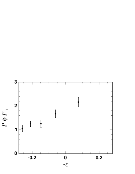
Figure 10: Plot of form factor $f^{+}$ extracted from BaBar experimental data multiplied by a function $P\phi$ as a function of $z$. It seems to be consistent with almost linear behavior in $z$. Figures from  [61].

Fermilab collaboration is carrying out an analysis based on Becher-Hill’s idea [63].

7.2 all-to-all propagators for heavy-light meson

TrinLat collaborations proposed to construct all-to-all propagators by combining low mode averaging [66], [22] and random noise vector technique. The noise should be diluted in time, spin and color sources. They have shown that their all-to-all propagator is particularly useful for the heavy-light propagator with 20 eigen modes and single random source per dilution for each configuration. This method seems very promising. More experience in large volume is needed.

8 Summary

Experimental data are offering us a chance to overconstrain CKM. Basic quantities such as decay constant, the bag parameter, form factors , b quark masses are important in many ways. Several different heavy quark formalism are useful for precision calculation are studied. New theoretical or calculation methods are proposed to give better accuracy.

References

- [1] A. Abulencia et al. [CDF Collaboration], arXiv:hep-ex/0609040.
- [2] K. Ikado et al., arXiv:hep-ex/0604018.
- [3] A. X. El-Khadra, A. S. Kronfeld and P. B. Mackenzie, Phys. Rev. D 55, 3933 (1997) [arXiv:hep-lat/9604004].
- [4] S. Aoki, Y. Kuramashi and S. i. Tominaga, Prog. Theor. Phys. 109, 383 (2003) [arXiv:hep-lat/0107009].
- [5] M. A. Nobes and H. D. Trottier, “Progress in automated perturbation theory for heavy quark physics,” Nucl. Phys. Proc. Suppl. 129, 355 (2004) [arXiv:hep-lat/0309086].
- [6] H. W. Lin and N. H. Christ, PoS LAT2005, 225 (2006) [arXiv:hep-lat/0510111].
- [7] H-W. Lin and N. Christ, these proceedings.
- [8] G.M. de Divitiis et al., M. Guagnelli, R. Petronzio, N. Tantalo and F. Palombi, “Heavy quark masses in the continuum limit of lattice QCD,” Nucl. Phys. B 675, 309 (2003) [arXiv: hep-lat/0305018].
- [9] G. M. de Divitiis, M. Guagnelli, F. Palombi, R. Petronzio and N. Tantalo, “Heavy-light decay constants in the continuum limit of lattice QCD,” Nucl. Phys. B 672, 372 (2003) [arXiv:hep-lat/0307005].
- [10] J. Heitger and R. Sommer [ALPHA Collaboration], “Non-perturbative heavy quark effective theory,” JHEP 0402, 022 (2004) [arXiv:hep-lat/0310035].
- [11] D. Guazzini, R. Sommer and N. Tantalo, These proceedings, POS(LAT2006)084 “m/b and f(Bs) from a combination of HQET and QCD,” arXiv:hep-lat/0609065.
- [12] A. Juttner and J. Rolf [ALPHA Collaboration], “A precise determination of the decay constant of the D/s-meson in quenched QCD,” Phys. Lett. B 560, 59 (2003) [arXiv:hep-lat/0302016].
- [13] M. Della Morte, S. Durr, J. Heitger, H. Molke, J. Rolf, A. Shindler and R. Sommer [ALPHA Collaboration], Phys. Lett. B 581, 93 (2004) [Erratum-ibid. B 612, 313 (2005)] [arXiv:hep-lat/0307021].
- [14] J. Heitger, M. Kurth and R. Sommer [ALPHA Collaboration], “Non-perturbative renormalization of the static axial current in quenched Nucl. Phys. B 669, 173 (2003) [arXiv:hep-lat/0302019].
- [15] J. Rolf et al. [ALPHA Collaboration], “Towards a precision computation of F(B/s) in quenched QCD,” Nucl. Phys. Proc. Suppl. 129, 322 (2004) [arXiv:hep-lat/0309072].
- [16] H. W. Lin, S. Ohta, A. Soni and N. Yamada, arXiv:hep-lat/0607035.
- [17] Y. Aoki et al., “The kaon B-parameter from quenched domain-wall QCD,” Phys. Rev. D 73, 094507 (2006) [arXiv:hep-lat/0508011].
- [18] T. W. Chiu, T. H. Hsieh, J. Y. Lee, P. H. Liu and H. J. Chang, PoS LAT2005, 041 (2006) [arXiv:hep-lat/0509172].
- [19] T. W. Chiu, T. H. Hsieh, J. Y. Lee, P. H. Liu and H. J. Chang, Phys. Lett. B 624, 31 (2005) [arXiv:hep-ph/0506266].
- [20] J. Simone’s poster, these proceedings.
- [21] M. Della Morte, P. Fritzsch, J Heitger, private commnunications from J. Heitger in preparing my plenary talk.
- [22] L. Giusti, P. Hernandez, M. Laine, P. Weisz and H. Wittig, “Low-energy couplings of QCD from current correlators near the chiral limit,” JHEP 0404, 013 (2004) [arXiv:hep-lat/0402002].
- [23] C. W. Bernard et al., “Lattice determination of heavy-light decay constants,” Phys. Rev. Lett. 81, 4812 (1998) [arXiv:hep-ph/9806412].
- [24] A. X. El-Khadra et al., A. S. Kronfeld, P. B. Mackenzie, S. M. Ryan and J. N. Simone, “B and D meson decay constants in lattice QCD,” Phys. Rev. D 58, 014506 (1998) [arXiv:hep-ph/9711426].
- [25] L. Lellouch and C. J. D. Lin [UKQCD Collaboration], “Standard model matrix elements for neutral B meson mixing and associated decay constants,” Phys. Rev. D 64, 094501 (2001) [arXiv:hep-ph/0011086].
- [26] C. Bernard et al. [MILC Collaboration], “Lattice calculation of heavy-light decay constants with two flavors of dynamical quarks,” Phys. Rev. D 66, 094501 (2002) [arXiv:hep-lat/0206016].
- [27] K. I. Ishikawa et al. [JLQCD Collaboration], “B meson leptonic decay constant with quenched lattice NRQCD,” Phys. Rev. D 61, 074501 (2000) [arXiv:hep-lat/9905036].
- [28] S. Aoki et al. [JLQCD Collaboration], “B0 anti-B0 mixing in unquenched lattice QCD,” Phys. Rev. Lett. 91, 212001 (2003) [arXiv:hep-ph/0307039].
- [29] A. Ali Khan et al. [CP-PACS Collaboration], “B meson decay constant from two-flavor lattice QCD with non-relativistic heavy quarks,” Phys. Rev. D 64, 054504 (2001) [arXiv:hep-lat/0103020].
- [30] A. Gray et al. [HPQCD Collaboration], “The B meson decay constant from unquenched lattice QCD,” Phys. Rev. Lett. 95, 212001 (2005) [arXiv:hep-lat/0507015].
- [31] A. Ali Khan et al. [CP-PACS Collaboration], “Decay constants of B and D mesons from improved relativistic lattice QCD with two flavours of sea quarks,” Phys. Rev. D 64, 034505 (2001) [arXiv:hep-lat/0010009].
- [32] V. Gadiyak and O. Loktik, “Lattice calculation of SU(3) flavor breaking ratios in B0 - anti-B0 Phys. Rev. D 72, 114504 (2005) [arXiv:hep-lat/0509075].
- [33] B. Grinstein et al., “Chiral perturbation theory for f D(s) / f D and B B(s) / B B,” Nucl. Phys. B 380, 369 (1992) [arXiv:hep-ph/9204207].
- [34] M. Wingate et al., C. T. H. Davies, A. Gray, G. P. Lepage and J. Shigemitsu, “The B/s and D/s decay constants in 3 flavor lattice QCD,” Phys. Rev. Lett. 92, 162001 (2004) [arXiv:hep-ph/0311130].
- [35] C. Aubin and C. Bernard, “Staggered chiral perturbation theory for heavy-light mesons,” Phys. Rev. D 73, 014515 (2006) [arXiv:hep-lat/0510088].
- [36] J. Shigemitsu et al, these proceedings.
- [37] D. Becirevic, V. Gimenez, G. Martinelli, M. Papinutto and J. Reyes, “B-parameters of the complete set of matrix elements of Delta(B) = 2 JHEP 0204, 025 (2002) [arXiv:hep-lat/0110091].
- [38] S. Hashimoto, K. I. Ishikawa, T. Onogi, M. Sakamoto, N. Tsutsui and N. Yamada, “Renormalization of the Delta(B) = 2 four-quark operators in lattice Phys. Rev. D 62, 114502 (2000) [arXiv:hep-lat/0004022].
- [39] S. Aoki et al. [JLQCD Collaboration], “B0 - anti-B0 mixing in quenched lattice QCD. ((U)) ((W)),” Phys. Rev. D 67, 014506 (2003) [arXiv:hep-lat/0208038].
- [40] E. Gulez, A. Gray, M. Wingate, C. T. H. Davies, G. P. Lepage and J. Shigemitsu, “B meson semileptonic form factors from unquenched lattice QCD,” Phys. Rev. D 73, 074502 (2006) [arXiv:hep-lat/0601021].
- [41] M. Okamoto et al. [Fermilab Lattice Collaboration], “Semileptonic D pi / K and B pi / D decays in 2+1 flavor lattice QCD,” arXiv:hep-lat/0409116.
- [42] Heavy Flavor Averaging Group, http://www.slac.stanford.edu/xorg/hfag.
- [43] J. Shigemitsu et al. [HPQCD Collaboration], “Semileptonic B decays with N(f) = 2+1 dynamical quarks,” arXiv:hep-lat/0408019.
- [44] K. C. Bowler et al. [UKQCD Collaboration], “Improved B pi l nu/l form factors from the lattice,” Phys. Lett. B 486, 111 (2000) [arXiv:hep-lat/9911011].
- [45] A. Abada et al., D. Becirevic, P. Boucaud, J. P. Leroy, V. Lubicz and F. Mescia, “Heavy light semileptonic decays of pseudoscalar mesons from lattice QCD,” Nucl. Phys. B 619, 565 (2001) [arXiv:hep-lat/0011065].
- [46] A. X. El-Khadra et al., A. S. Kronfeld, P. B. Mackenzie, S. M. Ryan and J. N. Simone, “The semileptonic decays B pi l nu and D pi l nu from lattice QCD,” Phys. Rev. D 64, 014502 (2001) [arXiv:hep-ph/0101023].
- [47] S. Aoki et al. [JLQCD Collaboration], “Differential decay rate of B pi l nu semileptonic decay with lattice NRQCD,” Phys. Rev. D 64, 114505 (2001) [arXiv:hep-lat/0106024].
- [48] S. B. Athar et al. [CLEO Collaboration], “Study of the q**2 dependence of B pi l nu and B rho (omega) l nu decay and extraction of V(ub),” Phys. Rev. D 68, 072003 (2003) [arXiv:hep-ex/0304019].
- [49] A. S. Kronfeld and J. N. Simone, Phys. Lett. B 490, 228 (2000) [Erratum-ibid. B 495, 441 (2000)] [arXiv:hep-ph/0006345].
- [50] Talk by E. Freeland, these proceedings.
- [51] G. Martinelli and C. T. Sachrajda, “Computation of the b-quark mass with perturbative matching at the next-to-next-to-leading order,” Nucl. Phys. B 559, 429 (1999) [arXiv:hep-lat/9812001].
- [52] M. Della Morte, N. Garron, R. Sommer and M. Papinutto, PoS LAT2005, 224 (2006) [arXiv:hep-lat/0509173].
- [53] F. Di Renzo and L. Scorzato, “The N(f) = 2 residual mass in perturbative lattice-HQET for an improved determination of the m(b)(MS-bar)(m(b)(MS-bar)),” arXiv:hep-lat/0408015.
- [54] C. McNeile, C. Michael and G. Thompson [UKQCD Collaboration], “An unquenched lattice QCD calculation of the mass of the bottom quark,” Phys. Lett. B 600, 77 (2004) [arXiv:hep-lat/0408025].
- [55] A. Gray, I. Allison, C. T. H. Davies, E. Gulez, G. P. Lepage, J. Shigemitsu and M. Wingate, “The Upsilon spectrum and m(b) from full lattice QCD,” Phys. Rev. D 72, 094507 (2005) [arXiv:hep-lat/0507013].
- [56] M. Nobes and H. Trottier, PoS LAT2005, 209 (2006) [arXiv:hep-lat/0509128].
- [57] O. Buchmuller and H. Flacher, “Fits to moment measurements from B –¿ X/c l nu and B –¿ X/s gamma decays Phys. Rev. D 73, 073008 (2006) [arXiv:hep-ph/0507253].
- [58] L. Lellouch, “Lattice-Constrained Unitarity Bounds for Decays,” Nucl. Phys. B 479, 353 (1996) [arXiv:hep-ph/9509358].
- [59] M. Fukunaga and T. Onogi, “A model independent determination of —V(ub)— using the global q**2 dependence of the dispersive bounds on the B –¿ pi l nu form factors,” Phys. Rev. D 71, 034506 (2005) [arXiv:hep-lat/0408037].
- [60] T. Becher and R. J. Hill, “Comment on form factor shape and extraction of —V(ub)— from B –¿ pi l Phys. Lett. B 633, 61 (2006) [arXiv:hep-ph/0509090].
- [61] R. J. Hill, “The modern description of semileptonic meson form factors,” eConf C060409, 027 (2006) [arXiv:hep-ph/0606023].
- [62] M. C. Arnesen, B. Grinstein, I. Z. Rothstein and I. W. Stewart, “A precision model independent determination of —V(ub)— from B –¿ pi e nu,” Phys. Rev. Lett. 95, 071802 (2005) [arXiv:hep-ph/0504209].
- [63] . R. Van de Water, these proceedings.
- [64] J. Foley, K. Jimmy Juge, A. O’Cais, M. Peardon, S. M. Ryan and J. I. Skullerud, “Practical all-to-all propagators for lattice QCD,” Comput. Phys. Commun. 172, 145 (2005) [arXiv:hep-lat/0505023].
- [65] S. Ryan, these proceedings.
- [66] T. A. DeGrand and U. M. Heller [MILC collaboration], “Witten-Veneziano relation, quenched QCD, and overlap fermions,” Phys. Rev. D 65, 114501 (2002) [arXiv:hep-lat/0202001].
- [67] A. Ali Khan et al., S. Collins, C. T. H. Davies, C. Morningstar, J. Shigemitsu and J. H. Sloan, “B meson decay constants from NRQCD,” Phys. Lett. B 427, 132 (1998) [arXiv:hep-lat/9801038].
- [68] S. Aoki et al. [JLQCD Collaboration], Phys. Rev. Lett. 80, 5711 (1998).
- [69] D. Becirevic et al., P. Boucaud, J. P. Leroy, V. Lubicz, G. Martinelli, F. Mescia and F. Rapuano, “Non-perturbatively improved heavy-light mesons: Masses and decay constants,” Phys. Rev. D 60, 074501 (1999) [arXiv:hep-lat/9811003].
- [70] D. Becirevic et al., D. Meloni, A. Retico, V. Gimenez, L. Giusti, V. Lubicz and G. Martinelli, “B0 anti-B0 mixing and decay constants with the non-perturbatively improved action,” Nucl. Phys. B 618, 241 (2001) [arXiv:hep-lat/0002025].
- [71] K. C. Bowler et al. L. Del Debbio, J. M. Flynn, G. N. Lacagnina, V. I. Lesk, C. M. Maynard and D. G. Richards [UKQCD Collaboration], “Decay constants of B and D mesons from non-perturbatively improved lattice QCD,” Nucl. Phys. B 619, 507 (2001) [arXiv:hep-lat/0007020].