Recent progress in finite temperature lattice QCD

Abstract:

I review recent progress in the determination of the QCD phase diagram at finite temperature, in investigations of the nature of the transition or crossover from the hadronic phase to the quark-gluon plasma phase and in the determination of the equation of state. This talk will focus on results at zero chemical potential.

1 Introduction

In the past few years our understanding of QCD at finite temperature has advanced considerably, due to improvements in the lattice discretizations (use of improved actions), improvements in the simulation algorithms, and increases in computational resources. A sketch of our present understanding of the QCD phase diagram in the $m_{ud}-m_{s}$ plane is shown in Fig. 1.

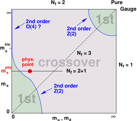
Figure 1: Sketch of the QCD phase diagram in the $m_{ud}-m_{s}$ plane.

In this talk I review recent progress in the determination of the QCD phase diagram at finite temperature and zero baryon density, in investigations of the nature of the transition or crossover from the hadronic phase at low temperatures to the quark-gluon plasma (QGP) phase at high temperatures and in the determination of the equation of state (EOS). For earlier recent reviews see Refs. [1], while a summary of other properties of the high-temperature phase is given in the talk by T. Hatsuda [2].

2 Simulation choices and improvements

As in any numerical simulation, for finite temperature studies one must makes choices of the action and parameters to be simulated. The most important choice, for dynamical fermion simulations, is the choice of fermion action, each of which has advantages and drawbacks. To weigh those we recall that the finite temperature transition or crossover is driven, for small quark masses, by the restoration of chiral symmetry in the high temperature phase.

(i) Wilson-type fermions, including clover fermions, have the advantage that they are local (in fact “ultralocal”) for any number of fermions, while the fermion determinant is positive for even numbers of fermions. Their big disadvantage is that the chiral symmetry is explicitly broken and the chiral limit therefore not protected. This makes the study of chiral symmetry restoration cumbersome and difficult. It becomes really meaningful only in the continuum limit.

(ii) Staggered fermions have the advantage that they have a (remnant) chiral symmetry. The chiral limit is thus protected. In addition, they are comparatively cheap to simulate. The main disadvantage of staggered fermions is the need to use the “fourth root trick” when the desired number of fermions of a given mass is not a multiple of four.

(iii) Overlap and domain wall fermions (at least for sufficiently large fifth dimension $L_{s}$) have the advantage of good chiral symmetry and the protection of the chiral limit, and of being local for any number of fermions (at least for sufficiently small lattice spacing $a$). Furthermore, for overlap fermions, the fermion determinant is positive for any number of fermions [3]. The disadvantage of these chiral fermion discretizations is that they are expensive to simulate. This problem is acerbated by the fact that one might need lattices with $N_{t}\geq 8$ to have lattice spacings small enough in the transition/crossover region for the fermion action to be sufficiently local. In judging this drawback, one should keep in mind that, for the computation of the EOS, for example, the scaling of the costs of a simulation is worse, by a factor $\sim a^{-4}$, than for typical zero temperature simulations, because the observable, obtained from the difference of a finite and a zero temperature simulation, decreases, in lattice units, as $a^{4}$, while the error decreases much slower.

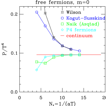
Figure 2: The pressure for free fermions with various fermion discretizations versus $N_{t}$, from Ref. [7].

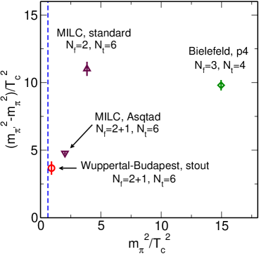
Figure 3: The pion mass splitting, $(m^{\prime 2}_{\pi}-m^{2}_{\pi})/T^{2}_{c}$ as function of $m^{2}_{\pi}/T^{2}_{c}$ at the lattice spacing corresponding to the finite temperature transition/crossover point, from Ref. [6].

Most of the recent dynamical fermion thermodynamics simulations have used improved versions of staggered fermions. The improvement aims to reduce taste symmetry breaking, by using some version of “smeared” or “fattened” gauge links in the nearest neighbor hopping term. This is done for all three versions currently under investigation, p4 (Bielefeld, RBC-Bielefeld) [4], asqtad (MILC) [5] and stout-link (Wuppertal-Budapest) [6]. The first two also aim to improve the dispersion relation, which implies improved behavior of thermodynamic quantities in the high temperature limit (i.e., for free fermions) by including three-hop terms: straight, the Naik term, for asqtad, and “knight moves” for p4. For free fermions, and hence in the high temperature limit, the link fattening becomes inoperative. Thus stout-link fermions act like standard staggered fermions, and asqtad fermions like Naik fermions. The two forms of improvement are illustrated in Figs. 3 and 3.

The other major advance, in the last couple of years, has come from the algorithmic side. Because of the fractional power of the fermion determinant, needed for the fourth-root trick, the usual, exact HMC algorithm [8] can not be used. Instead, the inexact hybrid R algorithm [9], with stepsize errors of ${\cal O}(\epsilon^{2})$, was employed. This obstacle was recently overcome with the invention of the exact RHMC algorithm [10]. As discussed in the talk by M. Clark [11] the RHMC algorithm is not only exact but allows various other improvements – multiple time-step integration schemes, multiple pseudofermion fields, etc. – that can speed up the simulations by factors of 2 up to 8 compared to the R algorithm.

A couple of exploratory studies with Wilson-type fermions were presented at this conference, using a hypercube action [12] and with twisted-mass Wilson fermions [13]. But in the rest of this talk I will concentrate on simulations with (improved) staggered fermions. For the purpose of this talk the validity of the fourth-root trick, discussed in detail by S. Sharpe [14], will be assumed.

3 The phase diagram

3.1 The physical point

Determining the nature of the finite temperature transition or crossover at the physical point is not only of interest in its own right, but has implications on the possible phase diagram with finite chemical potential (see e.g. the talks by C. Schmidt [15] and M. Stephanov[16]). The Wuppertal-Budapest group [17] made a systematic investigation using stout-link improved fermions and the exact RHMC algorithm. They used a physical strange quark mass and physical (degenerate) light quark masses. The chiral susceptibility for $N_{t}=4$ and $6$ and various volumes is shown in Fig. 4. It shows no sign of increasing with volume as would be expected for a genuine phase transition, indicating existence of only a crossover.

Figure 4: The chiral susceptibility for $N_{t}=4$ (left) and $N_{t}=6$ (right) and various volumes, from Ref. [17].

A definite statement, however, needs an extrapolation to the continuum and infinite volume limits. For a meaningful extrapolation renormalized observables have to be considered. The Wuppertal-Budapest group does this by subtracting the $T=0$ value, $\Delta\chi=\chi(T)-\chi(T=0)$, to cancel a potential additive divergence, and then multiplies with $m_{q}^{2}$ to obtain an RG invariant observable. This is then extrapolated to the continuum limit for fixed aspect ratio $N_{s}/N_{t}=3,4$ and $5$, see Fig. 5.

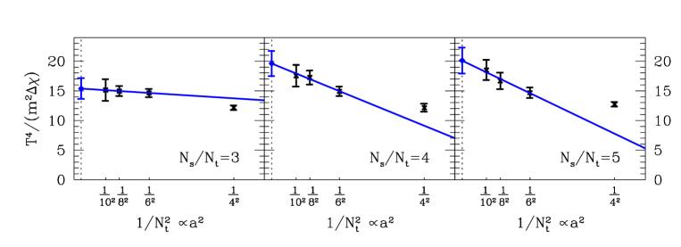
Figure 5: The continuum extrapolation of $T^{4}/(m_{q}^{2}\Delta\chi)$ for fixed aspect ratio $N_{s}/N_{t}=3,4$ and $5$, from Ref. [17].

The resulting continuum renormalized susceptibility stays finite and non-zero in the infinite volume limit. It would diverge for a genuine phase transition. Hence we now have convincing evidence that, in nature, QCD has a crossover at finite temperature and zero baryon chemical potential.

3.2 The second order boundary line

De Forcrand and Philipsen mapped out the second order critical line that separates the first order region at small quark masses from the crossover region at intermediate quark masses in the $m_{ud}-m_{s}$ plane of the phase diagram [18]. They used standard, i.e., unimproved, staggered fermions and the exact RHMC algorithm.

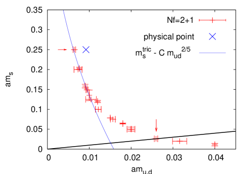
Figure 6: Determination of the second order boundary line between the first order and crossover regions in the $m_{ud}-m_{s}$ plane, from Ref. [18].

At fixed $am_{s}$ they determined the location of the second order point, as function of $am_{ud}$, by requiring that the Binder cummulant, $B_{4}(m_{ud}^{crit})$ attain its critical Ising value, $\simeq 1.6$. The locations, with errors, are shown in Fig. 6. The arrows in the plot indicate parameters values at which zero-temperature simulations were performed to determine meson masses and lattice spacing. De Forcrand and Philipsen found

• For the physical strange quark mass, the second order boundary occurs at non-vanishing $m_{ud}^{crit}<m_{ud}^{phys}$, i.e., the physical point is in the crossover region, in agreement with the result of the Wuppertal-Budapest group.

• The critical line is consistent with $m_{s}^{crit}(m_{ud})=m_{s}^{tric}-cm_{ud}^{2/5}$, i.e., the behavior that is expected if a tricritical point exists.

One should emphasize that these results are most likely qualitative, only. Unimproved staggered fermions were used on lattices with $N_{t}=4$, were the lattice spacing in the crossover/transition region is quite large, $a\sim 0.27$ fm. Therefore lattice effects could be significant. For example, at the second order critical point for three degenerate flavors, de Forcrand and Philipsen find $m_{\pi}/m_{\rho}=0.304(2)$, whereas the Bielefeld group, using p4 fermions, concluded that [19] $m_{\pi}/m_{\rho}<0.18$, the physical value of the mass ratio. For additional results with three degenerate flavors see also the contribution by Cheng [20].

3.3 Massless 2 flavor $\chi$QCD

Kogut and Sinclair continued their study of massless $N_{f}=2$ $\chi$QCD on $N_{t}=8$ lattices with $N_{s}=12,16$ and $24$ [21]. $\chi$QCD contains an irrelevant chiral 4-fermion interaction, which makes the fermion matrix non-singular in the limit of zero (bare) quark mass while preserving the chiral symmetry of the Lagrangian, thus enabling the study of spontaneous chiral symmetry breaking in the massless limit. For numerical simulations, the 4-fermion interaction is made quadratic in the fermions by introducing an auxiliary $(\sigma,\pi)$ field.

Kogut and Sinclair used (standard) staggered fermions which, at finite lattice spacing have a $U(1)\times U(1)$ chiral symmetry, expected to be spontaneously broken to $U(1)$. Hence, if the chiral symmetry restoration transition is second order, one expects the transition to be in the 3-d $O(2)$ universality class. Therefore, one wants to compare to the 3-d $O(2)$ spin model. However, the magnetization of the $O(2)$ spin model has large finite size effects, as seen in Fig. 7 (left). Hence, instead of comparing to infinite volume $O(2)$ behavior, Kogut and Sinclair compare to finite volume behavior for a “best matched size”. The strategy, thus, is to find the volume for which the $O(2)$ magnetization gives the best fit

$$\langle\bar{\psi}\psi(\beta)\rangle=b\;\langle M(a(\beta-\beta_{c})+T_{c})\rangle\qquad\quad i.e.\quad 1/J=T=a(\beta-\beta_{c})+T_{c}~{}.$$ (1)

of the chiral condensate, for a given QCD lattice size.

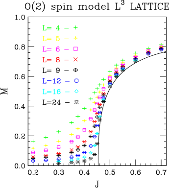
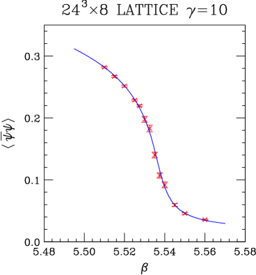
Figure 7: The magnetization of the $O(2)$ spin model in the transition region for various volumes (left) and an example of a best volume fit of $\langle\bar{\psi}\psi\rangle$ to the $O(2)$ spin model magnetization (right), from Ref. [21].

Such fits work well, see Fig. 7 (right), strongly suggesting that the $\chi$QCD data are compatible with the $O(2)$ spin model. The corresponding $O(2)$ volumes are small, $6^{3}$ for $16^{3}\times 8$ and $8^{3}$ for $24^{3}\times 8$. Thus, one should not attempt comparisons with large volume critical behavior. Kogut and Sinclair find, in retrospect, that such fits also work for their earlier $N_{t}=6$ data. Hence the conclusions of their earlier work, Ref. [22], should be modified accordingly.

3.4 2 flavor LQCD with KS quarks at $N_{t}=4$

The Pisa group [23] continued their investigation of the phase transition of $N_{f}=2$ QCD with standard staggered quarks at $N_{t}=4$. To check their previous results [24], obtained with the inexact R-algorithm they performed comparisons with the exact RHMC algorithm. They found that the systematic ${\cal O}(\epsilon^{2})$ step-size errors are comparable to the statistical ones.

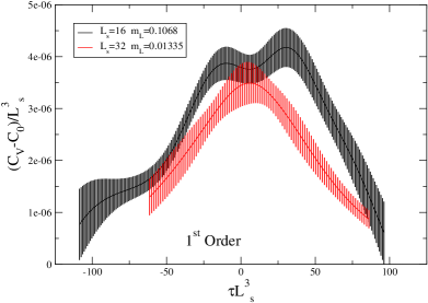
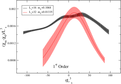
Figure 8: Test of first order finite volume scaling with $m_{L}L^{3}$ kept constant, from Ref. [23].

They then tested their hypothesis of a first order transition with a finite size scaling study of the specific heat, $C_{V}$, and chiral susceptibility, $\chi_{m}$, with the scaling variable $m_{L}L^{y_{h}}$ kept constant for the choice $y_{h}=3$, the value for a first order transition, see Fig. 8. The specific heat scales nicely, but not the chiral susceptibility. They speculate that the reason for the latter might be the large mass needed for the smaller volume, $am_{L=16}=0.1068$.

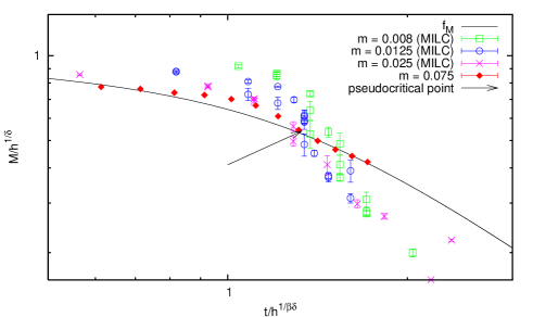
Figure 9: Comparison of $N_{f}=2$ QCD data with staggered fermions at $N_{t}=4$ to the $O(4)$ scaling function, from Ref. [25].

On the other hand, T. Mendes [25] recently compared previous data by the MILC collaboration [26] and her own new data at a heavier mass, $am=0.075$, with the (infinite volume) $O(4)$ scaling function, as shown in Fig. 9. Mendes inferred that the scaling works quite well, especially at the heavier mass.

I would conclude that the issue of the order of the phase transition for 2-flavor QCD, even with staggered fermions at $N_{t}=4$, and certainly in the continuum limit, remains an open question.

3.5 $T_{c}$ for full QCD

The RBC-Bielefeld collaboration [27, 28] has recently performed a systematic study of the crossover temperature in full QCD, i.e., physical strange quark mass, and degenerate light up and down quark masses, $m_{l}$. They used p4 fermions and the exact RHMC algorithm for simulations with $N_{t}=4$ and $6$, several light quark masses $m_{l}$, and fairly large volumes, $2\leq N_{s}/N_{t}\leq 4$.

For each simulation parameter set, they located the crossover point from the peak position of the chiral and Polyakov loop susceptibilities. The two peak positions appeared to coincide at large volume, suggesting that the crossovers for deconfinement and chiral symmetry restoration occur simultaneously. So the authors averaged over the two determinations at finite volume. $T_{c}$, in units of $r_{0}^{-1}$ is shown in Fig. 11 as function of $m_{PS}r_{0}$. The data at finite lattice spacing, $a\propto 1/N_{t}$, and unphysical light quark masses are then extrapolated to the continuum limit and physical point, given by $m_{PS}r_{0}=0.321(5)$ — $r_{0}$ was taken from Ref. [29]: $r_{0}=0.469(7)$ fm — using the form

$$(T_{c}r_{0})_{m_{l},N_{t}}=T_{c}r_{0}+A(m_{PS}r_{0})^{d}+B/N_{t}^{2}~{}.$$ (2)

Here, $d=1.08$ would be expected for a second order phase transition (in the $O(4)$ universality class) and $d=2$, i.e., a linear dependence on $m_{l}$, for a first order transition. At the physical point they find $T_{c}r_{0}=0.457(7)^{+8}_{-3}$, with the second error coming from using $d=2$ and $d=1$ in the extrapolation.

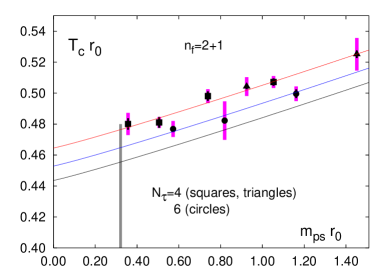
Figure 10: $T_{c}$ in units of $r_{0}^{-1}$ as function of $m_{PS}r_{0}$, from Ref. [27]. The vertical line shows the location of the physical value.

Figure 11: Recent lattice determinations of $T_{c}$, collected by P. Petreczky in Ref. [30].

In physical units, the transition/crossover temperature is $T_{c}=192(7)(4)\;{\rm Me\!V}\$. This is about 12% larger than the value obtained by the MILC collaboration, using asqtad fermions, the R-algorithm, lattices with $N_{t}=4,6,8$ and $N_{s}/N_{t}=2$, and a combined chiral/continuum limit extrapolation as in eq. (2). The MILC collaboration obtained $T_{c}=169(10)(4)\;{\rm Me\!V}\$ [7]. While they worked in units of the scale $r_{1}$, the conversion to physical units was done with compatible values and does not contribute to the disagreement. A collection of recent determinations of $T_{c}$, assembled by P. Petreczky in Ref. [30], is shown in Fig.  11.

4 The equation of state

After establishing the phase diagram, including the order and nature of the phase transitions and/or crossovers, one would like to understand the nature of the different phases. One of the basic quantities for this is the equation of state (EOS), the pressure $p(T)$, the entropy density $s(T)=dp(T)/dT$ and the energy density $\epsilon(T)=Ts(T)-p(T)$. Besides its intrinsic interest as a fundamental property of QCD, the EOS is of phenomenological interest. For example, it is an import input in hydrodynamical models of the QGP, often used to try to interpret results from heavy-ion collision experiments, such as the observed elliptic flow. For a quantitative understanding, obviously, a quantitative understanding of the EOS is necessary.

4.1 Low temperature behavior

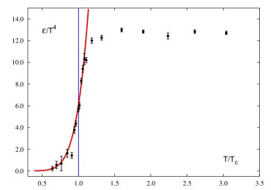
Figure 12: Comparison of the EOS from lattice simulations with a hadron resonance gas model with masses adjusted to the lattice quark masses used, from Ref. [31].

In the low temperature hadronic phase, the excitations are weakly interacting hadrons, including all resonances. This suggests that a hadron resonance gas model (HRG) should give a good description of the EOS. This was recently tested by a comparison with lattice data using p4-fermions and $N_{t}=4$ [31]. Since the light quark mass used was larger than the physical light quark mass, the hadron masses of the HRG where adjusted to match those on the lattice. With this adjustment the HRG works surprisingly well, even around the crossover temperature, as can be seen in Fig. 12.

4.2 The EOS at high temperatures

At (very) high temperatures the running coupling $g(T)$ vanishes (logarithmically in $T$), and one expects that the EOS should be computable in perturbation theory. PT, though, is afflicted with infrared divergences, requiring resummation of certain classes of diagrams, giving e.g. an ${\cal O}(g^{3})$ and an ${\cal O}(g^{5})$ contribution. At ${\cal O}(g^{6})$ the IR divergences cause all orders of PT to contribute, so that this order needs to be computed non-perturbatively. The last perturbative order, $g^{6}\log(1/g)$ has recently been computed using the technique of dimensional reduction [32].

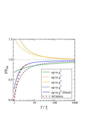
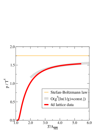
Figure 13: The pure gauge EOS in perturbation theory and the comparison with LGT data, from Refs. [32, 33].

The convergence, for pure gauge theory, is illustrated in Fig. 13. While the convergence is questionable, with fitting the unknown, non-perturbative $c_{6}g^{6}$ term to (pure gauge) LQCD results for $T>3T_{c}$, good agreement can be found [33]. The EOS, at high temperature, is thus reasonably well understood. The approach to the Stefan-Boltzmann (SB) limit is rather slow, due to the slow, only logarithmic vanishing of $g(T)$ with increasing temperature.

The high temperature behavior of pure gauge LGT in $2+1$ dimensions was recently investigated in detail [34]. In $2+1$-$d$, the dimensionless ratio $g^{2}/T$ serves as the running coupling that vanishes at high temperatures. Since the interaction measure (the trace anomaly) vanishes for free gluons, one expects

$$\frac{\epsilon-2p}{T^{3}}\simeq\frac{g^{2}}{T}~{}f\left(\log\frac{T}{g^{2}}\right)~{}.$$ (3)

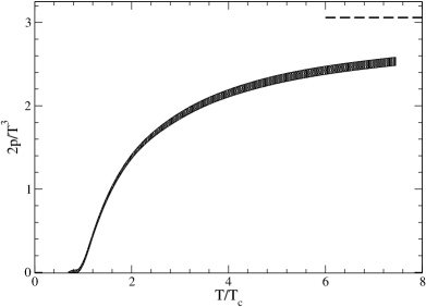
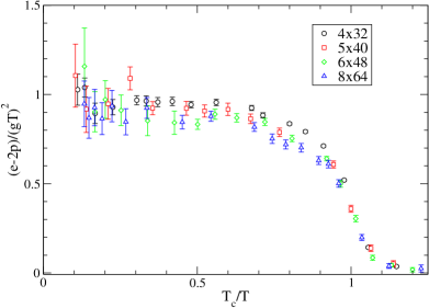
Figure 14: The pressure (left) and the interaction measure, scaled to leading perturbative behavior, (right) for purge gauge LGT in $2+1$ dimensions, from Ref. [34].

Fig. 14 shows pressure and interaction measure, scaled to the leading perturbative behavior. The data nicely confirm that $(\epsilon-2p)/(gT)^{2}$ approaches a constant at high temperature. The EOS is, again, well understood at high temperature, increasing our confidence in out understanding of the $3+1$-$D$ theory. Due to the faster running of the coupling, the pressure around $T\sim 2T_{c}$ is even farther from the SB limit than for $3+1$-$d$ QCD.

4.3 The EOS around the transition/crossover region

While the EOS is well understood and modeled at low and high temperatures the non-perturbative input from lattice calculations is needed to determine the EOS at intermediate temperatures, i.e., in the transition/crossover region. It is also needed, as we have seen, to calibrate the high temperature description — via the fit of the ${\cal O}(g^{6})$ term — and to check the range of validity of the HRG model at low temperatures.

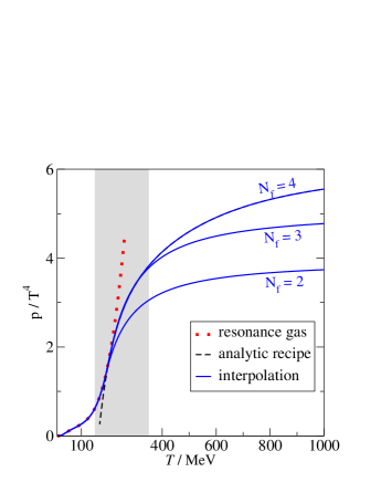
Figure 15: Quark mass effects from NLO perturbation theory on a “phenomenological modeling” of the EOS [33] (see text).

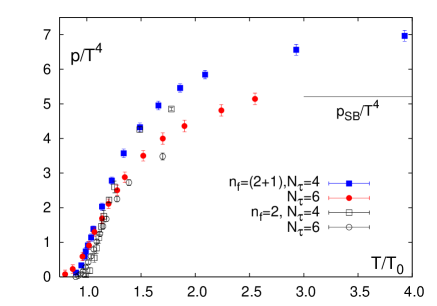
Figure 16: Quark mass effects in the lattice EOS with staggered quarks. $N_{f}=2$ standard staggered data are from Refs. [35, 36] and $N_{f}=2+1$ stout-link data from Ref. [6].

This intermediate temperature range is also the region where the effect of the strange quark, with $m_{s}/T_{c}\sim{\cal O}(1)$, and even of the charm quark, become visible. This can be seen in Fig. 16 which shows the quark mass effects incorporated as NLO perturbative corrections to a phenomenological modeling of the EOS based on the HRG, pure gauge lattice results and perturbation theory [33], and Fig. 16, which compares lattice results for staggered quarks with $N_{f}=2$ [35, 36] and $N_{f}=2+1$ [6] flavors. The effect of the strange quark becomes clearly noticeable around $T\approx 1.5T_{c}$ and the effect of the charm quark above $T\sim 3T_{c}$.

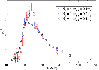
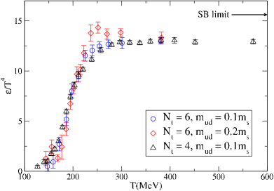
Figure 17: The interaction measure (left) and the energy density (right) from $2+1$ flavor simulations with asqtad fermions along two lines of constant physics [37].

There have been two recent computations of the EOS in full QCD, on the path to a determination in the continuum limit, both using $N_{t}=4$ and $6$ lattices. The first, using stout-link improved fermions and the exact RHMC algorithm, appeared in Ref. [6]. Since stout-link fermions do not have an improved high temperature behavior, the authors of Ref. [6] applied an a-posteriori tree-level correction factor $c_{cont}/c_{N_{t}}=0.571$ and $0.663$ for $N_{t}=4$ and $6$ to correct for the tree level ${\cal O}(a^{2})$ lattice effects (see difference in the data presented in Fig. 16 and Fig. 18 (right)).

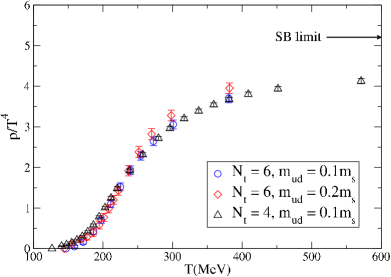
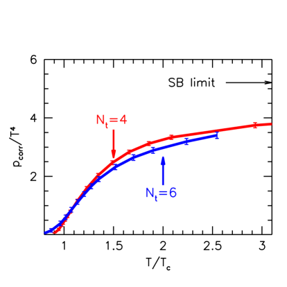
Figure 18: The pressure with asqtad fermions, from Ref. [37], (left) and with stout-link fermions, corrected for tree-level lattice effects, from Ref. [6], (right) for full QCD simulations.

The second, by the MILC collaboration, described in more detail in the contribution by L. Levkova [37], uses asqtad fermions. For the most part, configurations generated earlier with the R-algorithm [7] were analyzed. The major effort, over the last six months, concerned an estimate of, and correction for, the step-size errors induced by the R-algorithm as described in more detail in the contribution by L. Levkova [37].

The preliminary, step-size corrected results along two different lines of constant physics, with $m_{l}=0.2m_{s}$ and $m_{l}=0.1m_{s}$, and two $N_{t}$’s, $4$ and $6$ for the latter case, for the interaction measure and the energy density are shown in Fig. 17. Overall, light quark mass and lattice spacing effects appear to be fairly small. The pressure along these lines of constant physics is compared with the result from stout-link fermions of Ref. [6] in Fig. 18. With appropriate caveats, the two determinations agree reasonably well.

A reliable continuum extrapolation of the EOS for full QCD should become possible in the not too distant future. Certainly, simulations with $N_{t}=8$ are needed, and a repeat of the asqtad fermion simulations for $N_{t}=4$ and $6$ with the exact RHMC algorithm would be desirable.

5 Other results

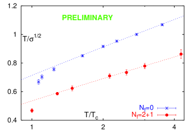
Figure 19: The space-like string tension for pure gauge theory and for $2+1$ flavor QCD, from Ref. [28].

At high temperature, one expects dimensional reduction for QCD to work well, especially in the chromomagnetic sector. The dimensionful 3-d gauge coupling is given by $g_{3}^{2}=g^{2}(T)T$, and the fermions, to leading order, affect only the running of $g(T)$ – higher order corrections can be included, see Ref. [42]. This proposition was studied recently by measuring the spatial string tension in $2+1$ flavor QCD with p4 fermions [28] and comparing to pure gauge results, as shown in Fig. 19. The comparison can be quantified by fitting $\sqrt{\sigma}=c_{3}g_{3}^{2}=c_{3}g^{2}(T)T$, with $c_{3}=0.587(41)$ for $2+1$ flavor QCD, as compared to $c_{3}=0.566(13)$ for 4-d SU(3) pure gauge theory [43] and $c_{3}=0.553(1)$ for the 3-d theory [44]. Similarly, for 2-flavor QCD with clover fermions, Ukita reported $c_{3}=0.54(6)$ [45], compatible with these results.

Several other interesting results in finite temperature lattice gauge theory appeared during the last year or were presented at this conference. These include a study of the dynamics of the phase transition in pure SU(3) lattice gauge theory [38], indications of a non-trivial fixed point in finite temperature U(1) lattice gauge theory [39], a suggestion that the center vortex field is the field that becomes massless at the deconfinement transition of pure gauge SU(2) theory [40], and impressively accurate results for two-color strong coupling QCD with staggered fermions at finite temperature, and finite chemical potential, with a novel cluster algorithm [41].

6 Conclusions

During the last year simulations with improved staggered fermions have produced convincing evidence that in nature, at zero baryon density, there is a crossover from the hadronic phase to the quark-gluon plasma phase, rather than a genuine phase transition [17]. A new determination found a crossover temperature of $192(8)\;{\rm Me\!V}$ [27], some 10-15% larger than earlier estimates. Both results need confirmation from other groups and, in particular, from other fermion discretizations.

Progress has been made in the computation of the EOS for full QCD at intermediate temperatures, around the crossover region, where model and perturbative calculations are unreliable. $N_{t}=8$ results, though, are needed for controlled continuum extrapolations.

Much remains to be done in understanding the quark-gluon plasma phase in the vicinity of the crossover. For example, determinations of transport coefficients and response functions would be very desirable.

Acknowledgments: Thanks to all who provided information and figures for this review, and thanks to my colleagues from the MILC collaboration and to Frithjof Karsch for numerous discussions on the subject covered here.

References

- [1] P. Petreczky, Nucl. Phys. Proc. Suppl. 140, 78 (2005) [hep-lat/0409139]; O. Philipsen, Proc. Sci. LAT2005, 016 (2005) [hep-lat/0510077].
- [2] T. Hatsuda, these proceedings.
- [3] A. Bode, U.M. Heller, R.G. Edwards, and R. Narayanan, in “Structure of the Vacuum”, Kluwer Academic 2000, pg 65 [hep-lat/9912043]; R.G. Edwards, U.M. Heller and R. Narayanan, Phys. Rev. D 59, 094510 (1999) [hep-lat/9811030].
- [4] U.M. Heller, F. Karsch and B. Sturm, Phys. Rev. D 60, 114502 (1999) [hep-lat/9901010].
- [5] Kostas Orginos, Doug Toussaint and R.L. Sugar, Phys. Rev. D 60, 054503 (1999) [hep-lat/9903032]; G.P. Lepage, Phys. Rev. D 59, 074502 (1999) [hep-lat/9809157].
- [6] Y. Aoki, Z. Fodor, S.D. Katz, and K.K. Szabo, J. High Energy Phys. 01, 089 (2006) [hep-lat/0510084].
- [7] MILC Collaboration: C. Bernard, et al., Phys. Rev. D 71, 034504 (2005) [hep-lat/0405029].
- [8] S. Duane, A.D. Kennedy, B.J. Pendleton, and D. Roweth, Phys. Lett. B 195, 216 (1987).
- [9] S.A. Gottlieb, W. Liu, D. Toussaint, R.L. Renken, and R.L. Sugar, Phys. Rev. D 35, 2531 (1987).
- [10] M.A. Clark, B. Joo and A.D. Kennedy, Nucl. Phys. Proc. Suppl. 119, 1015 (2003) [hep-lat/0209035]; M.A. Clark and A.D. Kennedy, Nucl. Phys. Proc. Suppl. 129, 850 (2004) [hep-lat/0309084]; M.A. Clark, A.D. Kennedy and Z. Sroczynski, Nucl. Phys. Proc. Suppl. 140, 835 (2005) [hep-lat/0409133].
- [11] M. Clark, these proceedings.
- [12] S. Shcheredin, these proceedings.
- [13] . M-P. Lombardo, these proceedings.
- [14] S. Sharpe, these proceedings.
- [15] C. Schmidt, these proceedings.
- [16] M. Stephanov, these proceedings.
- [17] K. Szabo, these proceedings.
- [18] Philippe de Forcrand and Owe Philipsen, hep-lat/0607017.
- [19] F. Karsch, E. Laermann and C. Schmidt, Phys. Lett. B 520, 41 (2001) [hep-lat/0107020].
- [20] M. Cheng, these proceedings.
- [21] J.B. Kogut and D.K. Sinclair, Phys. Rev. D 73, 074512 (2006) [hep-lat/0603021].
- [22] J.B. Kogut and D.K. Sinclair, Phys. Lett. B 492, 228 (2000) [hep-lat/0005007]; Phys. Rev. D 64, 034508 (2001) [hep-lat/0104011].
- [23] C. Pica, these proceedings.
- [24] M. D’Elia, A. Di Giacomo and C. Pica, Phys. Rev. D 72, 114510 (2005) [hep-lat/0503030].
- [25] T. Mendes, to appear in the Proceedings of the “I Latin American Workshop in High Energy Phenomenology”, Porto Alegre, Brazil, December 2005, hep-lat/0609035.
- [26] MILC Collaboration: C. Bernard, et al., Phys. Rev. D 61, 054503 (2000) [hep-lat/9908008].
- [27] M. Cheng, et al., hep-lat/0608013, to appear in Phys. Rev. D;
- [28] T. Umeda, these proceedings.
- [29] A. Gray, et al., Phys. Rev. D 72, 094507 (2005) [hep-lat/0507013].
- [30] P. Petreczky, hep-lat/0609040.
- [31] F. Karsch, K. Redlich and A. Tawfik, Eur. Phys. J. C 29, 549 (2003) [hep-ph/0303108]
- [32] K. Kajantie, M. Laine, K. Rummukainen, and Y. Schröder, Phys. Rev. D 67, 105008 (2003) [hep-ph/0211321].
- [33] Mikko Laine and York Schröder, Phys. Rev. D 73, 085009 (2006) [hep-ph/0603048].
- [34] P. Bialas, L. Daniel, A. Morel, and B. Petersson, hep-lat/0606019.
- [35] T. Blum, Steven Gottlieb, Leo Karkkainen, D. Toussaint, Phys. Rev. D 51, 5153 (1995) [hep-lat/9410014].
- [36] MILC Collaboration: C.W. Bernard, et al., Phys. Rev. D 55, 6861 (1997) [hep-lat/9612025].
- [37] MILC Collaboration: C. Bernard, et al., these proceedings.
- [38] A. Bazavov, these proceedings.
- [39] B.A. Berg, these proceedings.
- [40] K. Langfeld, G. Schulze and H. Reinhardt, Phys. Rev. Lett. 95, 221601 (2005) [hep-lat/0508007].
- [41] Shailesh Chandrasekharan and Fu-Jiun Jiang, Phys. Rev. D 74, 014506 (2006) [hep-lat/0602031].
- [42] M. Laine and Y. Schröder, Proc. Sci. LAT2005, 180 (2005) [hep-lat/0509104].
- [43] G. Boyd et al., Nucl. Phys. B 469, 419 (1996) [hep-lat/9602007].
- [44] B. Lucini and M. Teper, Phys. Rev. D 66, 097502 (2002) [hep-lat/0206027].
- [45] N. Ukita et al., these proceedings.