PoS(LAT2006)021
BNL-NT-06/40

Lattice QCD at finite density

Abstract:

I discuss different approaches to finite density lattice QCD.  In particular, I focus on the structure of the phase diagram and discuss attempts to determine the location of the critical end-point. Recent results on the transiton line as function of the chemical potential ($T_{c}(\mu_{q})$) are reviewed. Along the transition line, hadronic fluctuations have been calculated, which can be used to characterize properties of the Quark Gluon plasma and eventually can also help to identify the location of the critical end-point in the QCD phase diagram on the lattice and in heavy ion experiments. Furthermore, I comment on the structure of the phase diagram at large $\mu_{q}$.

1 Introduction

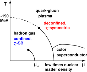
Figure 1: Sketch of the QCD phase diagram.

Lattice QCD currently is the only quantitative approach to finite temperature QCD based on first principle calculation. For a recent review see [1]. At non zero density however, lattice QCD is harmed by the sign problem ever since its inception. The Fermion matrix becomes complex and can not be interpreted as a probability distribution. Hence straight forward Monte Carlo simulations become impossible. For a detailed description of the sign problem in the epsilon regime see [2].

During the last few years a lot of progress has been made to circumvent the sign problem for small values of $\mu_{q}/T$, where $\mu_{q}$ is the quark chemical potential and $T$ the temperature. This progress helps to understand the physics relevant for heavy ion collisions and eventually will clarify the existence/location of the critical end-point in the QCD phase diagram. In Fig. 1 a sketch of the QCD phase diagram in the $T$-$\mu$ plane is shown. Lattice QCD calculations provide more and more evidence that the QCD transition at $\mu_{q}=0$ is not a phase transition in the thermodynamic sense, but a smooth crossover. Further evidence was seen recently in [3]. Nevertheless, one can define a transition temperature $T_{c}$ by the peak position of the chiral susceptibility. As a function of the quark chemical potential the line of transition temperatures ($T_{c}(\mu_{q})$) is smoothly connected to a critical end-point in the ($T,\mu_{q}$)-diagram. For larger chemical potentials the QCD transition is expected to be first order. At high densities, several color superconducting phases are expected.

The rest of the article is organized as follows: in Sec. 2 I will briefly recall different methods which have been used so far to calculate thermodynamic observables at non zero chemical potential. In Sec. 3 I will summarize current knowledge about the $\mu_{q}$-dependence of the critical temperature. I will continue with reviewing results on quark number fluctuations along the transition line (Sec. 4) and the critical point (Sec. 5). Finally I will discuss the physics beyond the critical point in Sec. 6.

2 Methods to extract information on the chemical potential dependence

2.1 Reweighting from the ($\mu=0$)-ensemble

On the lattice one has to choose several parameters to characterize a thermodynamic system. In addition to the number of lattice points in spacial and temporal directions, $N_{s},N_{t}$ respectively, we have to choose quark masses $m_{q}$, the coupling $\beta\equiv 6/g^{2}$ and the chemical potential $\mu_{q}$. Together these parameters define the lattice spacing $a$ and thus also the temperate $T\equiv 1/aN_{t}$ and volume $V\equiv(aN_{s})^{3}$ of the simulated system. A thermodynamic observable is calculated on the lattice as

$$\left<O\right>_{\beta,m_{q},\mu_{q}}=\frac{1}{Z(V,T)}\int{\mathcal{D}U}\;O\;\left[{\rm det}M(U;m_{q},\mu_{q})\right]^{N_{f}/4}\;\exp\{-\beta S_{G}(U)\}\quad.$$ (1)

Here $N_{f}$ is the number of dynamical fermions. The notation is written down for staggered fermions as the additional factor of $1/4$ in the power of the fermion determinant indicates. See [4] for a discussion of the “4th root trick” needed to calculate the staggered fermion determinant.

In principle it is possible to calculate the expectation value of the observable at the parameter set $p=\{\beta,m_{q},\mu_{q}\}$, from an ensemble generated at $p_{0}=\{\beta_{0},m_{q,0},\mu_{q,0}\}$. We have the identity

$$\left<O\right>_{p}=\left<O\;R(U;p,p_{0})\right>_{p_{0}}/\left<R(U;p,p_{0})\right>_{p_{0}}\quad,$$ (2)

where we define the reweighting factor $R$ as

$$R(U;p,p_{0})\equiv\left[{\rm det}M(U;p)/{\rm det}M(U;p_{0})\right]^{N_{f}/4}\;\exp\{-(\beta-\beta_{0})S_{G}\}\quad.$$ (3)

The reweighting method as a tool to perform extrapolation and interpolation in the gauge coupling $\beta$ goes back to [5]. For reweighting in the chemical potential it was first used by the Glasgow group [6]. However, since the overlap between the generated ensemble at $\mu_{q,0}=0$ and the target ensemble at $\mu_{q}>0$ exponentially decreases with increasing $\mu_{q}$, the method was successful only after it was generalized to a multi-parameter approach [7]. For $N_{t}=4$ lattices it was found that reweighting along the transition line $T_{c}(\mu_{q})$ works quite well up to $a\mu_{q}\raise 1.29167pt\hbox{$<$\kern-7.5pt\raise-4.73611pt\hbox{$\sim$}}0.3$ or equivalently for $\mu_{q}/T\raise 1.29167pt\hbox{$<$\kern-7.5pt\raise-4.73611pt\hbox{$\sim$}}1.2$.

In general the reweighting approach requires the evaluation of the fermion determinant on every configuration. As this is computationally demanding, one may consider to expand the reweighting factor given in Eq. (3) in terms of the chemical potential [8]. In this case the reweighting procedure is, however, only correct up to a certain order in $\mu_{q}/T$.

2.2 The Taylor expansion method

It is conceptually very simple to calculate the expansion coefficients of any observable $O$ (Eq. (1)) in a Taylor series around $\mu_{q}=0$:

$$O(\hat{\mu})=c_{0}+c_{1}\hat{\mu}+\frac{1}{2}c_{2}\hat{\mu}^{2}+\cdots\quad.$$ (4)

Since on the lattice all quantities are given in units of the lattice spacing ($a$), the expansion parameter is $\hat{\mu}\equiv a\mu_{q}=N_{t}^{-1}(\mu_{q}/T)$. This idea goes back to the first calculation of the quark number susceptibility [9]. The response of meson masses [10] as well as the pressure and further bulk thermodynamic quantities [11, 12, 13, 14] have been studied by this method. The first two nontrivial coefficients in Eq. (4) are given by

$$c_{1} = \left<\frac{\partial O}{\partial\hat{\mu}}\right>\!+\!\left<O\frac{\partial\ln\rm{det}M}{\partial\hat{\mu}}\right>$$ (5)

$$c_{2} = \left<\frac{\partial^{2}O}{\partial\hat{\mu}^{2}}\right>\!+\!2\left<\frac{\partial O}{\partial\hat{\mu}}\frac{\partial\ln\rm{det}M}{\partial\hat{\mu}}\right>\!+\!\left<O\frac{\partial^{2}\ln\rm{det}M}{\partial\hat{\mu}^{2}}\right>\!-\!\bigg{<}O\bigg{>}\left<\frac{\partial^{2}\ln\rm{det}M}{\partial\hat{\mu}^{2}}\right>\quad.$$

Besides derivatives of the observable itself, the calculation of derivatives of $\ln\rm{det}M$ with respect to $\hat{\mu}$ is required. The derivatives have to be taken at $\hat{\mu}_{0}=0$. Note that due to a symmetry of the partition function ($Z(\mu_{q})=Z(-\mu_{q}))$ all odd coefficients in Eq. (4) vanish identically. For the same reason we have $\left<\partial\ln\rm{det}M/\partial\hat{\mu}\right>=0$ at $\hat{\mu}=0$. We explicitly use this property in Eq. (5) to derive the expansion coefficients.

The advantages of this method are that expectations values only have to be evaluated at $\hat{\mu}=0$, i.e. calculations are not directly affected by the sign problem. Furthermore, all derivatives of the fermion determinant can be expressed in terms of traces by using the identity $\ln\rm{det}M=\rm{Tr}\ln M$. This enables the stochastic calculation of the expansion coefficients by the random noise method, which is much faster than a direct evaluation of the determinant. Moreover, the continuum and infinite volume extrapolations are well defined on a coefficient by coefficient basis.

On the other hand it is a priori not clear for how large $\mu/T$ the method works and how large the truncation errors are. Furthermore one is strictly limited by phase transitions, since phase transitions are connected with discontinuities or divergences. An estimation of the convergence radius of the series gives a lower bound on the applicability range and thus also a lower bound to the phase transition line in the $(T,\mu)$ plane (see the discussion in Sec. 5).

2.3 Analytic continuation

At imaginary chemical potentials, the fermion determinant is real and positive, thus simulations by standard Monte Carlo techniques are possible. Results on the imaginary $\hat{\mu}_{I}$ axis can be analytically continued to the real $\hat{\mu}_{R}$ axis. It is especially easy to convert a Taylor series in $\hat{\mu}_{I}$, expanded around $\hat{\mu}=0$, into a Taylor series in $\hat{\mu}_{R}$. Since the series has only even powers of $\hat{\mu}$, due to the the symmetry $Z(\hat{\mu})=Z(-\hat{\mu})$, one only has to switch the sign of every second coefficient ($c_{2}\rightarrow-c_{2},c_{6}\rightarrow-c_{6},\dots$). There is however another symmetry of the partition function which limits the analytic continuation. Due to the periodicity [15] $Z(\mu_{R},\mu_{I})=Z(\mu_{R},\mu_{I}+2\pi T/3)$ simulations with $\mu_{I}>0$ will only give access to the physical region $\mu_{R}\raise 1.29167pt\hbox{$<$\kern-7.5pt\raise-4.73611pt\hbox{$\sim$}}\pi T/3$. This method was used to map out the phase transition line [16]-[18]. One should note, that for this method neither an evaluation of the determinant, nor any of its derivatives is required. In order to determine the functional dependence of an observable on $\hat{\mu}_{R}$ one needs many different simulation points for several values of $\hat{\mu}_{I}$, to perform an analytic continuation using a certain Ansatz.

A demonstration of the imaginary chemical potential method is given in Fig. 3.

Figure 2: The chiral condensate as a function of $\hat{\mu}^{2}$, in $SU(2)$ gauge theory [19]. The solid lines are fits with different Ansätze to the data for $\hat{\mu}^{2}<0$.

Figure 3: Relation between the Baryon number and the chemical potential from the saddle point approximation, for different temperatures [27].

The method was applied to the case of 2-color QCD [19]. Here it is not only possible to calculate observables at $\hat{\mu}^{2}<0$, but also at $\hat{\mu}^{2}>0$, since 2-color QCD does not suffer from a sign problem. Thus one can explicitly check how far the extrapolation in $\hat{\mu}^{2}$ is valid and which type of Ansatz is especially well suited for the extrapolation. In general, extrapolations with rational functions seem to be better than extrapolations with polynomials [19, 20].

2.4 The canonical approach

The canonical partition function ($Z_{C}$) can be constructed by introducing a $\delta$-function into the grand canonical partition function which fixes the net number of quarks present in the system. Using an integral representation of the $\delta$-function one recognizes the integration parameter as an imaginary chemical potential. One finds

$$Z_{C}(T,Q=3B)=\frac{1}{2\pi}\int_{-\pi}^{\pi}{\rm d}\left(\frac{\mu_{I}}{T}\right)\;\exp\left\{-i3B\frac{\mu_{I}}{T}\right\}Z_{GC}(T,i\mu_{I})\quad.$$ (6)

Thus, the canonical partition functions are the coefficients of the Fourier expansion of the grand canonical partition function ($Z_{CG}$) in imaginary $\mu$. Here we have used the $2\pi T/3$ periodicity of the grand canonical partition function which as a consequence leads to the fact that the canonical partition functions vanish for non-integer values of the baryon number $B=3Q$.

The Fourier-coefficients can be computed exactly [26]. As for the reweighting method (2.1), the evaluation of the fermion determinant is required on every configuration. In fact the same method can be used, which is the calculation of all $6N_{s}^{3}$ eigenvalues of the so-called “reduced matrix” [7].

After having calculated the canonical partition functions, a relation between the chemical potential and the baryon number is needed, in order to explore the phase diagram in the $(T,\mu)$-plane. Such a relation can be obtained by using the saddle point approximation of the fugacity expansion (which is exact in the thermodynamic limit). One finds

$$\mu(\rho)=\frac{1}{3}\frac{\partial f(\rho)}{\partial\rho}\quad,$$ (7)

where $\rho=B/V$ is the baryon number density and $f(T,\rho)=-\frac{T}{V}{\rm log}Z_{C}(T,\rho)$ is the Helmhotz free energy density. For several different temperatures the saddle point approximation is shown in Fig. 3 [27]. Due to the computational costs the calculation have been performed on $6^{3}\times 4$ lattices, with $N_{f}=4$ flavors of staggered fermions. As can be seen from the “S”-shape of the curves, one can have more than one solution when solving for the baryon density $\rho$, at given $\mu$ and $T$. This reflects the nature of the transition in the four-flavor theory, which is of first order. By using a Maxwell construction, one is able to calculate the two densities $\rho_{1}(T)<\rho_{2}(T)$, giving the lower and upper boundary of the coexistence area, as well as the critical chemical potential $\mu_{B}^{crit}(T)$, as functions of the temperature.

2.5 The density of states method

An alternative to the importance sampling technique used in most Monte Carlo simulations is the density of states method. Here one reorders the path integral representation of the partition function in the following way: first expectation values with a constrained parameter will be calculated. I.e. one selected parameter ($\phi$) is fixed. Expectation values according to the usual grand canonical partition function ($Z_{GC}$) can then be recovered by the integral

$$<O>=\int d\phi\,\left<Of(U)\right>_{\phi}\rho(\phi)\left/\int d\phi\,\left<f(U)\right>_{\phi}\rho(\phi)\right.$$ (8)

where the density of states ($\rho$) is given by the constrained partition function:

$$\rho(x)\equiv Z_{\phi}(x)=\int\mathcal{D}U\,g(U)\,\delta(\phi-x)\quad.$$ (9)

Here $\left<~{}\right>_{\phi}$ denotes the expectation value with respect to the constrained partition function. In addition, the product of the weight functions $f,g$ has to equal the correct measure of $Z_{GC}$: $fg=\rm{det}M\cdot\exp\{-S_{G}\}$. The idea of reordering the partition functions is rather old and was used successfully for gauge theories [21] and QED with dynamical fermions [22]. For QCD the parameter $\phi$ is usually chosen to be the plaquette [23]: $\phi=P$. In [24], however, the DOS method was constructed for the complex phase ($\phi=\theta$). Within the random matrix model, the authors of [25] used the quark number density ($\phi=n_{q}$).

The advantages of this additional integration becomes clear, when choosing $\phi=P$ and $g(U)=1$. In this case $\rho(\phi)$ is independent of all simulation parameters. The observable can be calculated as a function of all values of the lattice coupling $\beta$. If one has stored all eigenvalues of the fermion matrix for all configurations, the observable can also be calculated as a function of quark mass ($m$) and number of flavors[23] ($N_{f}$).

Note that this method does not solve the sign problem. It is, however supposed to solve the overlap problem. Moreover, it is also possible to combine the DOS method, with the reweighting method 2.1, by reweighting the constrained expectation values in the case of $g(U)\neq 1$. For large reweighting distances an overlap problem is then introduced once again.

3 The transition line

Using any of the methods presented above, the calculation of the transition line $T_{c}(\mu_{q})$ is possible. This has been done for many systems, which differ in the number of quark flavors, quark masses, physical volume and lattice spacing. This makes a comparison of different methods difficult. The case of $N_{f}=4$, $m/T=0.2$ and $N_{t}=4$, however, has been studied extensively with almost all methods. A comparison is given in Fig. 5 [27].

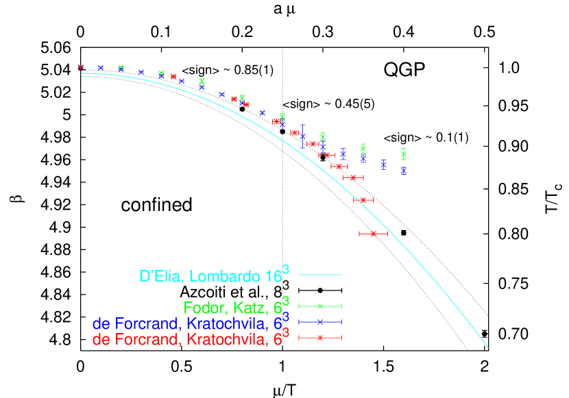
Figure 4: Comparison of the transition line $T_{c}(\mu)$ obtained from different methods. Plot from [27].

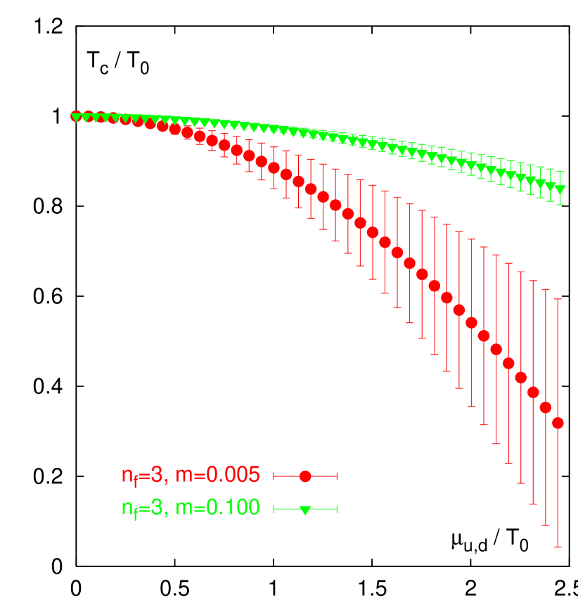
Figure 5: The mass dependence of the transition line for $N_{f}=3$ [29].

As one can see, the agreement between different methods is very good up to $a\mu_{q}\approx 0.3$ or equivalently $\mu_{q}/T\approx 1.2$. For larger chemical potential the two results from the reweighting method (Sec. 2.1), indicated as green and blue points, seem to stay above the other results. The reason could be the lack of overlap between the simulated and the reweighted ensemble.

Other results shown in Fig. 5 come from the imaginary chemical potential approach (Sec. 2.3), solid line, from a generalized imaginary chemical potential approach, black dots, and from the canonical approach (Sec. 2.4), red points. These results seem to be in agreement even for somewhat larger chemical potentials. However, the transition line from the canonical approach bends down at $\mu/T\approx 1.5$. Strong coupling calculations at $\beta=0$ [28] show that this is indeed necessary in order to match with the correct strong coupling limit.

To discuss the transition line a bit more quantitatively, one can expand $T_{c}(\mu_{q})$ in terms of the chemical potential

$$\frac{T_{c}(\mu_{q})}{T_{c}(0)}=1-t_{2}(N_{f},m_{q})\left(\frac{\mu_{q}}{\pi T}\right)^{2}+{\mathcal{O}}\left(\left(\frac{\mu_{q}}{\pi T}\right)^{4}\right)\quad.$$ (10)

In general the first non trivial coefficient $t_{2}$ will depend on the number of flavors and the quark masses as indicated above. Of course they will also be sensitive to finite volume and cut-off effects. One can, however, hope that for large physical volumes and small lattice spacings, i.e. $N_{s}/N_{t}>4$ and $N_{t}>4$, those effects are small. A detailed comparison of $t_{2}$ is given in Tab. 1.

$N_{f}$	$am$	$N_{s}$	$t_{2}$	Action	$\beta$-Function	Method	Reference
2	0.1	16	0.69(35)	p4	non-pert.	Taylor+Rew.	[8]
	0.032	6,8	0.500(54)	stag.	2-loop pert.	Imag.	[17]
3	0.1	16	0.247(59)	p4	non-pert.	Taylor+Rew.	[29]
	0.026	8,12,16	0.667(6)	stag.	2-loop pert.	Imag.	[39]
	0.005	16	1.13(45)	p4	non-pert.	Taylor+Rew.	[29]
4	0.05	16	1.86(2)	stag.	2-loop pert.	Imag.	[18]
2+1	0.0092,0.25	6-12	0.284(9)	stag.	non-pert.	Rew.	[34]

Table 1: Comparison of the first nontrivial coefficient $t_{2}$ in the Taylor expansion of the transition line. All results have been obtained with $N_{t}=4$.

In general, the curvature of the transition line becomes steeper for increasing number of flavors and decreasing quark masses. Two of the 3-flavor results which have been obtained with the p4-improved action [29] are shown in Fig. 5. In some cases it has also been possible to estimate the sub-leading coefficient $t_{4}$, which has been found to be very small or even negative. If an extrapolation with a Padé Ansatz is performed, the transition line tends to be steeper for high $\mu_{q}$ [20] compared to the truncated Taylor series and shows faster convergence.

We also note, that the calculation of $T_{c}(\mu_{q})$ has two parts. The first part involves the calculation of $\beta_{c}(\hat{\mu})$, the second one is the calculation of the lattice $\beta$-function ($a\partial\beta/\partial a$). Some of the results listed in Tab. 1 have been obtained by using the perturbative two-loop $\beta$-function, which has the tendency to underestimate the curvature of the critical line.

4 Hadronic fluctuations

Following the transition line into the non-zero chemical potential plane, quark number fluctuations $\chi_{q}$ belong to the most important observables. They will diverge at the critical end-point and thus provide an excellent signal for the existence and its location on the lattice and eventually may be detectable in heavy ion experiments. Hadronic fluctuations can be computed from Taylor expansion coefficients of the pressure with respect to the quark chemical potential:

$$\frac{p}{T^{4}}=\sum_{n=0}^{\infty}c_{n}(T)\left(\frac{\mu_{q}}{T}\right)^{n}\quad\mbox{with}\quad c_{n}(T)=\left.\frac{1}{n!}\frac{N_{t}^{3}}{N_{s}^{3}}\frac{\partial{\rm ln}Z}{\partial(\hat{\mu}N_{t})^{n}}\right|_{\hat{\mu}=0}\quad.$$ (11)

Due to the particle anti-particle symmetry ($\mu_{q}\leftrightarrow-\mu_{q}$) all odd coefficients vanish. Thus the first three non-zero coefficients are $c_{2}$, $c_{4}$, and $c_{6}$. They have been calculated in the case of two flavors of p4-improved staggered fermions, with $m_{q}/T=0.4$ [13] and are shown in Fig. 6.

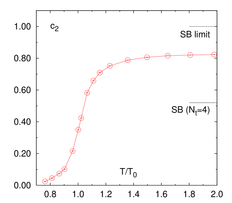
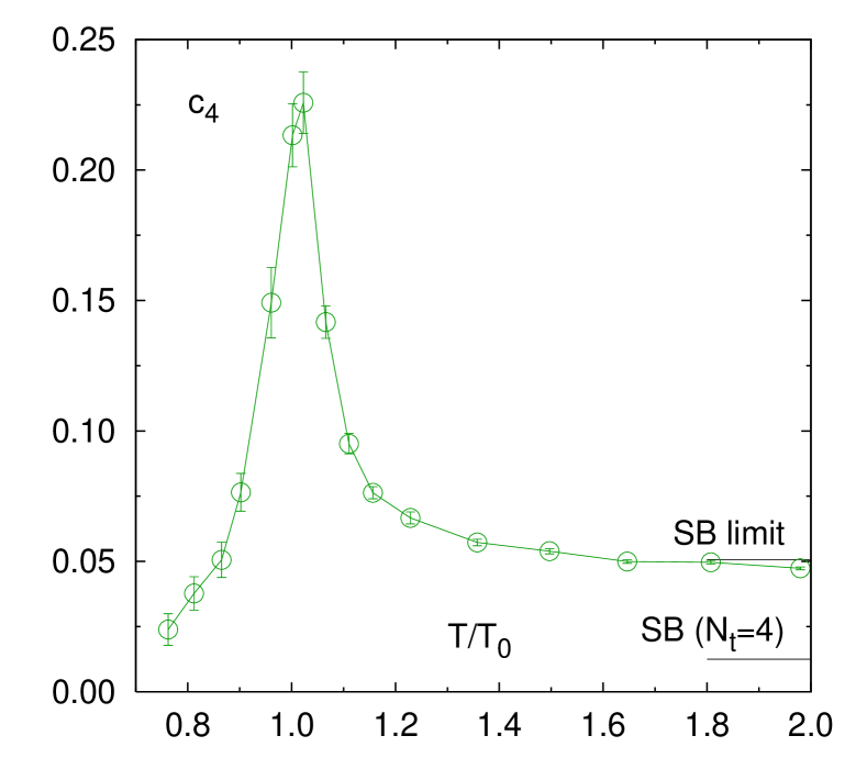
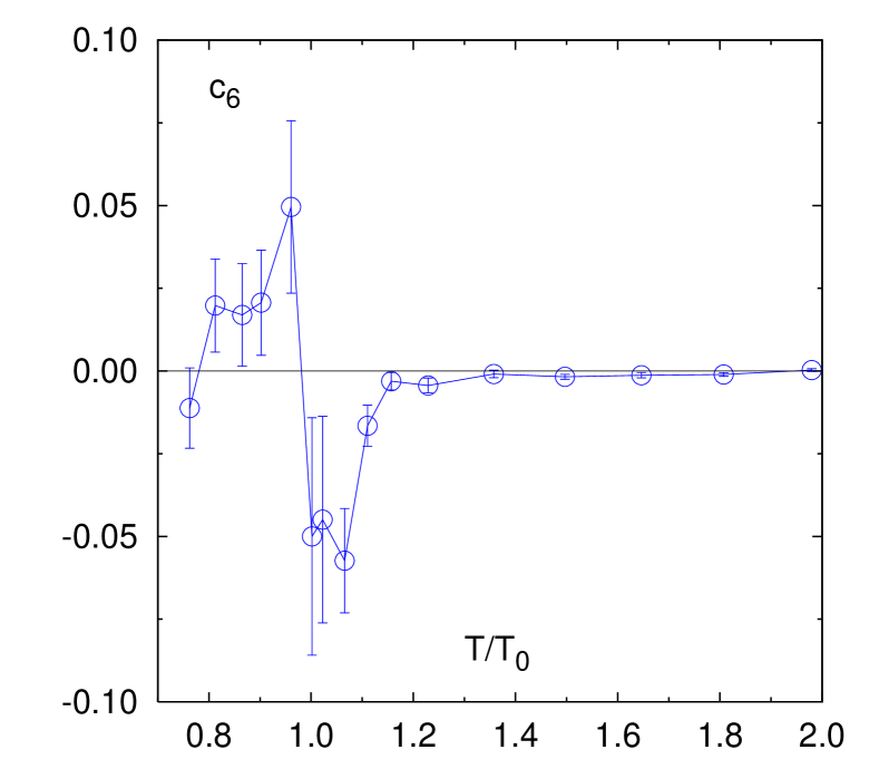
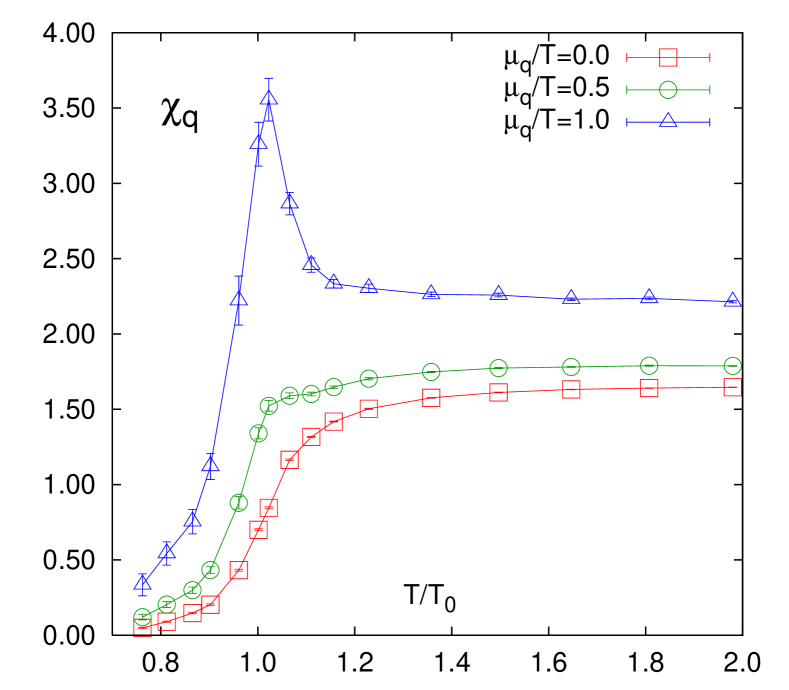
Figure 6: The Taylor expansion coefficients $c_{2}$, $c_{4}$ and $c_{6}$ of the pressure [13] and the quark number fluctuations $\chi_{q}$ for different values of the quark chemical potential.

Note that in the Taylor expansion of the pressure the up and down quark chemical potentials have been chosen to be equal. Having calculated the coefficients $c_{n}(T)$ one can construct the quark number density and quark number fluctuations

$$\frac{n_{q}}{T^{3}}=\sum_{n=2}^{\infty}nc_{n}(T)\left(\frac{\mu_{q}}{T}\right)^{n-1}\quad;\quad\frac{\chi_{q}}{T^{2}}=\sum_{n=2}^{\infty}n(n-1)c_{n}(T)\left(\frac{\mu_{q}}{T}\right)^{n-2}\quad.$$ (12)

Also shown in Fig. 6 are the quark number fluctuations for various values of the chemical potential. It is interesting to see that at $\mu_{q}=0$, the fluctuations $\chi_{q}$ show a rapid but monotonic increase at the transition temperature, whereas a cusp is developing at $T_{c}(\mu_{q})$ for $\mu_{q}>0$. This is a clear sign for approaching the critical end-point.

In the case of 2-flavor QCD, the quark number susceptibility is directly proportional to the baryon number fluctuation. Having two light quarks and one heavier strange quark, the situation is not that simple anymore. To match the situations realized in heavy ion collisions, one still wants to expand the pressure in terms of $\mu_{q}=\mu_{u}=\mu_{d}$, keeping the strange quark chemical potential zero ($\mu_{s}=0$). However, in order to analyze fluctuations of conserved quantum numbers, it appears to be more appropriate to perform a basis change going from the space of quark number fluctuations

$$\chi_{\alpha,\beta}=\left<n_{\alpha}n_{\beta}\right>-\left<n_{\alpha}\right>\left<n_{\beta}\right>\propto\frac{T}{V}\frac{\partial^{2}{\rm log}Z}{\partial\mu_{\alpha}\partial\mu_{\beta}}\quad,$$ (13)

where $\alpha,\beta\in\{u,d,s\}$ to the space of hadronic fluctuations, indicated by $\alpha,\beta\in\{I_{3},Y,B\}$ with $I_{3}$ being the third component of the isospin, $Y$ being the hypercharge and $B$ the baryon number. In Fig. 7 the diagonal susceptibilities $\chi_{I_{3},I_{3}}$, $\chi_{Y,Y}$ and $\chi_{B,B}$ as well as the off-diagonal susceptibility $\chi_{Y,B}$ are shown [30].

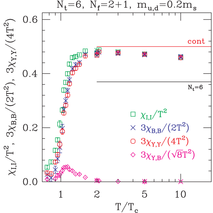
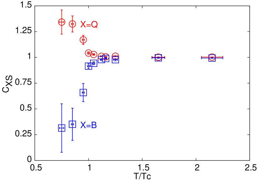
Figure 7: Different hadronic fluctuations [30] and the correlation between strangeness and baryon number, electric charge fluctuations respectively [31].

They have been measured by the MILC Collaboration with 2+1 flavor of Asqtad fermions on a $12^{3}\times 6$ lattice. The light quark mass is $m_{q}=0.2m_{s}$ where $m_{s}$ is the physical strange quark mass. The curves have been normalized such that the continuum Stefan-Boltzmann value is 0.5 for all of them. Qualitatively they show the same behavior as the diagonal quark number fluctuations, only the off-diagonal susceptibility $\chi_{Y,B}$ shows a cusp already at $\mu=0$. However, up to a minus sign also the off-diagonal quark susceptibility $\chi_{u,d}$ shows a cusp at $\mu=0$.

Furthermore, also fluctuations of other conserved quantities such as electric charge $Q$ have been computed. It is especially interesting to analyze the correlations between different conserved charges. Also shown in Fig. 7 are the correlations

$$C_{X,S}=\frac{\left<XS\right>-\left<X\right>\left<S\right>}{\left<S^{2}\right>-\left<X\right>^{2}}\quad,$$ (14)

where $S$ is the strangeness and the operator $X$ is either the electric charge ($X=Q$) or the baryon number ($X=B$) [31]. Such calculations have been performed on an $16^{3}\times 4$ lattice, using a standard staggered action. The two dynamical light quark masses yield $m_{\pi}/m_{\rho}=0.3$. The strange quark has been treated in the quenched approximation. The results show that above $T_{c}$ strangeness and electric charge or baryon number fluctuate independently. This is consistent with the quasi-particle picture of the Quark-Gluon-Plasma (QGP). However, below $T_{c}$, in the hadronic phase fluctuations are clearly correlated. These correlations are thus directly related to the degrees of freedom in the QGP. These are also clearly visible in the calculation of higher order cumulants of fluctuations [32].

5 The critical end-point

Locating the critical point is one of the most challenging tasks for lattice QCD at finite chemical potential. The first attempt to locate the critical point used the reweighting method [33]. For this calculation, 2+1 flavor of standard staggered fermions have been used at a pion mass of about 300 MeV and a kaon mass of about 500 MeV. Lattice sizes have, however, been rather small ($4^{3}\times 4$ - $8^{3}\times 4$). A critical chemical potential of $\mu_{B}^{crit}=725(35)$ was found. A second calculation [34], using again the reweighting method, with physical masses ($m_{\pi}=150$ MeV, $m_{K}=500$ MeV) and somewhat larger volume ($6^{3}\times 4$ - $12^{3}\times 4$), let to $\mu_{B}^{crit}=360(4)$ MeV.

When using the reweighting method for locating the critical point, the minima of the normalized partition function in the complex $\beta$-plane (Lee-Yang zeros) have to be determined

$$Z_{\rm norm}\equiv\left|\frac{Z(\beta_{\rm Re},\beta_{\rm Im},\mu)}{Z(\beta_{\rm Re},0,0)}\right|=\left|\left<e^{6i\beta N_{t}N_{s}^{3}\Delta S_{G}}e^{i\theta}e^{(N_{f}/4)({\rm lndet}M(\mu)-{\rm lndet}M(0))}\right>_{(\beta_{\rm Re},0,0)}\right|\quad.$$ (15)

In $SU(3)$ gauge theory, where we have $e^{i\theta}=1$, this can be done with high accuracy, which can be seen in Fig. 8 [35].

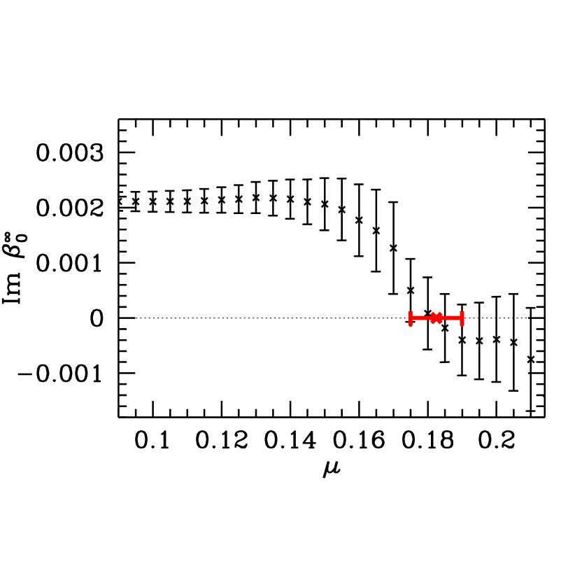
Figure 8: Lee-Yang Zeroes in the complex $\beta$ plane, in the case of $SU(3)$ gauge theory [35] (left) and the distance of the smallest Lee-Yang zero from the real axis as function of the chemical potential, in the case of full QCD [34] (right).

One can even identify a second Lee-Yang zero. In order to locate the critical point, one has to take the infinite volume limit and monitor the approach of the Lee-Yang zeros on the real axis. When the first Lee-Yang zero touches the real axis in the infinite volume limit, a critical point has been reached. In Fig. 8 this is shown for full QCD with physical masses [34]. In QCD with non-zero chemical potential the analysis of Lee-Yang zeros is, however, subtle [35]. For large volumes and chemical potentials the phase factor of the determinant $e^{i\theta}$ will force the Lee-Yang zero onto the real axis, which might lead to an underestimation of the critical point.

Another difficulty with the reweighting method at finite chemical potential has been pointed out in [36]. It was noted, that taking the fourth (or square) root of the determinant (which is necessary in order to simulate 2 or 1-flavor QCD with staggered fermions; see also [4]) could lead to phase ambiguities. This problem becomes acute when $\mu_{q}>m_{\pi}/2$.

All of the a above mentioned limitations are, however, irrelevant for the location of the critical point with the reweighting method if the critical point is located at small values of $\mu_{q}$.

Using the Taylor expansion coefficients of the pressure, it is also possible to estimate the location of the critical point. The convergence radius of the expansion is limited by the nearest singularity in the complex chemical potential plane. For each fixed temperature, the radius of convergence is given by

$$\rho=\lim_{n\to\infty}\rho_{n}=\lim_{n\to\infty}\sqrt{\left|\frac{c_{n}}{c_{n+2}}\right|}\quad.$$ (16)

Moreover, the sign of the coefficients $c_{n}$ gives information about the location of the singularity in the complex plane. If all coefficients are positive, the singularity is located on the real axis of the complex chemical potential plane. If the sign is strictly alternating, the singularity lies on the imaginary axis. For a detailed discussion see [37].

Having only a limited number of expansion coefficients, one can only estimate $\rho$. The hope is that the convergence of the $\rho_{n}$ will be fast. Indeed, a clustering of the $\rho_{n}$ is seen in the phase diagram, as shown in Fig. 9 [13].

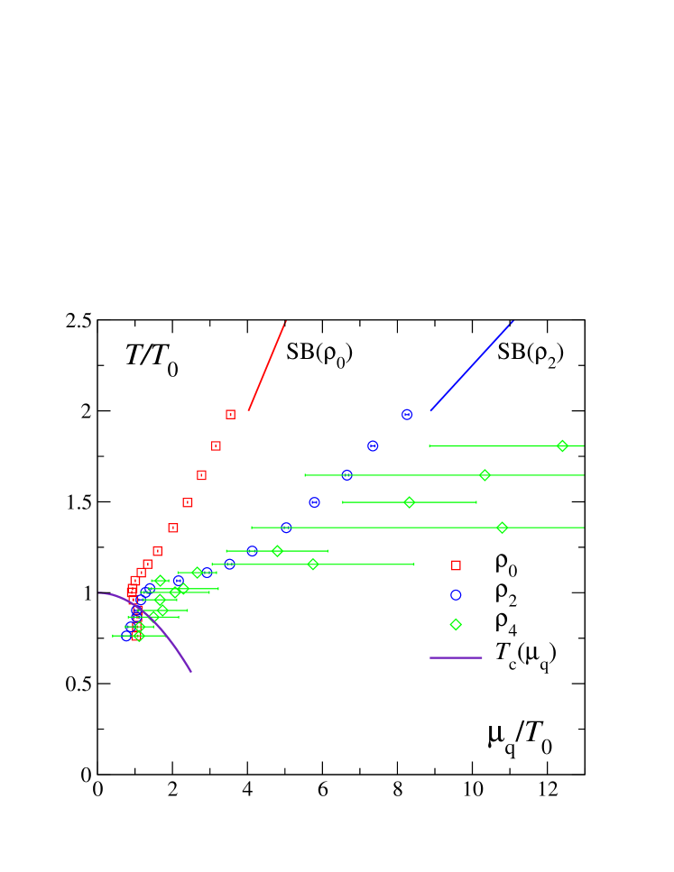
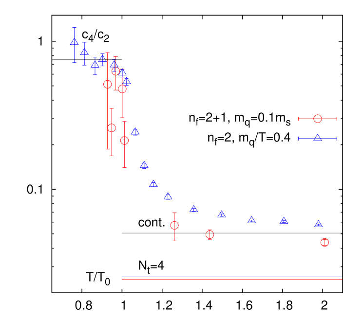
Figure 9: Estimates of the radius of convergence in the $(T,\mu_{q})$-plane (left), the ratio $c_{4}/c_{2}$ of the expansion coefficients (right).

This calculation, which has been performed with 2 flavors of p4 improved fermions and $m_{\pi}/m_{\rho}=0.7$, suggests a critical chemical potential of $\mu_{B}^{crit}\approx 500$ MeV. All calculated $\rho_{n}$ are, however, consistent (within statistical error) with the resonance gas model in the Boltzmann approximation, where the radius of convergence is infinity.

The authors of [38] have estimated the critical chemical potential from a Taylor expansion of the quark number susceptibility and find $\mu_{B}^{crit}\approx 180$ MeV. Two flavors of standard staggered fermions have been used on lattices up to $24^{3}\times 4$ and quark mass corresponding to $m_{\pi}/m_{\rho}=0.3$. The difference between the two estimates [13, 38] of the critical point is large. We note that the second estimate comes from the expansion coefficients of $\chi_{q}$. As can be seen from Eq. 12 this will result in a smaller $\rho_{n}$ for each fixed $n$. The limit $\lim_{n\to\infty}\rho_{n}$ is of course the same. For finite $n$, however, the estimate of $\mu_{B}^{crit}\approx 180$ MeV would correspond to $\mu_{B}^{crit}\approx 240$ MeV, when estimating the $\rho_{n}$ with coefficients of the same order from the expansion of the pressure. Nonetheless, the difference between the two estimates is still striking. The origin could be the difference in mass. However, preliminary results from the RBC-Bielefeld Collaboration, also shown in Fig. 9, do not indicate a strong mass dependence in $c_{4}/c_{2}=1/\rho_{2}^{2}$.

The critical point can also be studied directly at $\mu_{q}=0$. This can be done by tuning the quark masses carefully to a value where the critical chemical potential is $\mu_{B}^{crit}=0$. In the quark mass plane of two degenerate light quark and one strange quark, ($m_{u,d},m_{s}$)-plane, a line exists on which this condition is fulfilled. Starting from this line, one can define a surface of critical points in the 3-dimensional space of ($m_{u,d},m_{s},\mu_{q}$). On one site of the surface, the order of the QCD transition is first order (for smaller masses) on the other side the transition is only a smooth crossover. The line of critical points at $\mu_{q}=0$ has been computed for standard staggered fermions [39] as shown in Fig. 10.

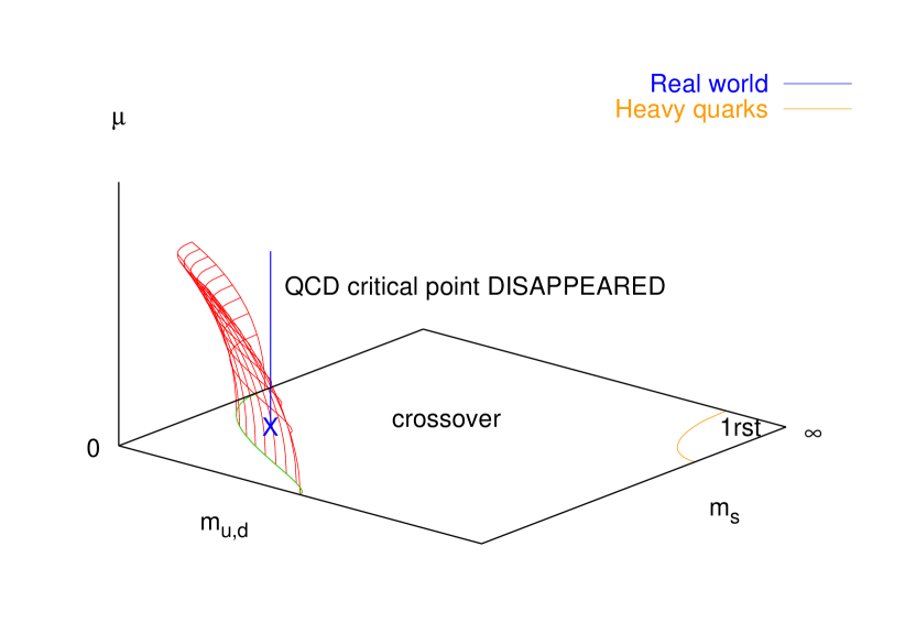
Figure 10: Line of critical points in the quark mass plane for $\mu_{B}=0$ and $i\mu_{B}=2.4T$ (left) and sketch of the surface of critical points as found in [39] (right).

For locating the critical points, the fourth order Binder cumulants of the chiral condensate have been calculated. Since the probability distribution of the order parameter is universal, also the value of its forth cumulant is a renormalization group invariant quantity which furthermore is volume independent at the critical point. From a calculation of cumulants at imaginary chemical potential the region of first order phase transitions was found to shrink as sketched in Fig. 10. This calculation has been performed with standard staggered fermions on an rather course lattices ($N_{t}=4$). If this result gets confirmed in the continuum limit it would put doubts on the existence of a critical point in QCD with physical masses. It is interesting to mention, that a shrinking region of first order transitions has also been found in the case if isospin chemical potential [41].

6 Beyond the critical point

Even more challenging than locating the critical point, is the study of the physics at high densities and low temperatures. One attempt to do so is a calculation using the density of states method [40]. Using four flavors of standard staggered fermions (i.e. taking the root of the determinant is no necessary), several simulation points in the $(\beta,\hat{\mu})$ plane have been chosen to generate phase quenched configurations by employing the method proposed in [42]. The lattice size has been $6^{3}\times 4$ and $6^{4}$. The quark mass was chosen to be $m/T=0.2$. The generation has been done with constrained plaquettes. In oder to do so, the $\delta$-function in Eq. 9 has been replaced by a sharply peaked Gaussian potential, which in practice means that the force term in the HMD-R algorithm had to be modified. In the notation used in Sec. 2.5 this would mean $\phi=P$, $g=|{\rm det}M|e^{-\beta S_{G}}$ and $f=e^{i\theta}$. For each simulation point, several runs have been performed with about 20 different values of the plaquette. By calculating the eigenvalues of the reduced matrix the phase of the determinant was calculated for each of those runs. By numerically calculating the integrals

$$\left<P\right>=\int dx\;x\rho(x)\left<{\rm cos}(\theta)\right>_{x}\quad\left<P^{2}\right>=\int dx\;x^{2}\rho(x)\left<{\rm cos}(\theta)\right>_{x}\quad,$$ (17)

we recover the grand canonical expectation value of the plaquette and its square. Here $\rho(x)$ is the density of states (Eq. 9), which has been measured by the integral method, usually used to calculate the pressure. The susceptibility of the plaquette is then given by the usual expression $\chi_{P}=\left<P^{2}\right>-\left<P\right>^{2}$. From the peak position of the plaquette susceptibility the phase diagram was calculated as shown in Fig. 11.

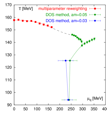
Figure 11: Phase diagram from the density of state method [39].

The scale was set by the Sommer radius $r_{0}$, measured on a $10^{3}\times 20$ lattice. We find a triple point, where three different phases seem to coexist. The phases show different plaquette expectation values. The triple point is located around $\mu_{q}^{\rm tri}\approx 300~{}\mbox{MeV}$, however its temperature ($T^{\rm tri}$) decreases from $T^{\rm tri}\approx 148\mbox{MeV}$ on the $6^{3}\times 4$ lattice to $T^{\rm tri}\approx 137\mbox{MeV}$ on the $6^{4}$ lattice. This shift reflects the relatively large cut-off effects one faces with standard staggered fermions and temporal extents of 4 and 6.

Also shown in Figure 11 are points from simulations with quark mass $m/T=1.2$. The phase boundary turned out to be — within our statistical uncertainties — independent of the mass.

References

- [1] U. M. Heller, to appear in PoS LAT2006, arXiv:hep-lat/0610114.
- [2] K. Splittorff, to appear in PoS LAT2006, arXiv:hep-lat/0610072.
-
[3]
Y. Aoki, G. Endrodi, Z. Fodor, S. Katz, K. Szabo,
Nature 443 (2006) 675;
K. Szabo et al., to appear in PoS LAT2006. - [4] S. R. Sharpe, to appear in PoS LAT2006, arXiv:hep-lat/0610094.
-
[5]
A. M. Ferrenberg and R. H. Swendsen,
Phys. Rev. Lett. 61 (1988) 2635;
Phys. Rev. Lett. 63 (1989) 1195. - [6] I. M. Barbour et al., Phys. Rev. D 56 (1997) 7063 .
- [7] Z. Fodor and S. Katz, Phys. Lett. B 534 (2002) 87.
- [8] C. R. Allton et al., Phys. Rev. D 66 (2002) 074507.
- [9] S. A. Gottlieb et al., Phys. Rev. D 38 (1988) 2888.
-
[10]
S. Choe et al. [QCD-TARO Collaboration],
Nucl. Phys. Proc. Suppl. 106 (2002) 462;
Phys. Rev. D 65 (2002) 054501; Nucl. Phys. A 698 (2002) 395. - [11] R. V. Gavai and S. Gupta, Phys. Rev. D 68 (2003) 034506.
- [12] C. R. Allton et al., Phys. Rev. D 68 (2003) 014507.
- [13] C. R. Allton et al., Phys. Rev. D 71 (2005) 054508.
- [14] S. Ejiri, F. Karsch, E. Laermann and C. Schmidt, Phys. Rev. D 73 (2006) 054506.
- [15] A. Roberge and N. Weiss, Nucl. Phys. B 275 (1986) 734.
- [16] P. de Forcrand and O. Philipsen, Nucl. Phys. B 673 (2003) 170.
- [17] P. de Forcrand and O. Philipsen, Nucl. Phys. B 642 (2002) 290.
- [18] M. D’Elia and M. P. Lombardo, Phys. Rev. D 67 (2003) 014505.
-
[19]
P. Giudice and A. Papa,
Phys. Rev. D 69 (2004) 094509;
Nucl. Phys. Proc. Suppl. 140 (2005) 529;
P. Cea, L. Cosmai, M. D’Elia and A. Papa, to appear in PoS LAT2006, arXiv:hep-lat/0610088. -
[20]
M. D’Elia and M. P. Lombardo,
Phys. Rev. D 70 (2004) 074509;
M. P. Lombardo, PoS LAT2005 (2006) 168 -
[21]
G. Bhanot et at.,
Phys. Lett. B 187 (1987) 381;
Phys. Lett. B 188 (1987) 246;
M.Karliner et al., Nucl. Phys. B 302 (1988) 204. - [22] V. Azcoiti, G. di Carlo and A. F. Grillo, Phys. Rev. Lett. 65 (1990) 2239.
- [23] X. Q. Luo, Mod. Phys. Lett. A 16 (2001) 1615.
- [24] A. Gocksch, Phys. Rev. Lett. 61 (1988) 2054.
- [25] J. Ambjorn et al., JHEP 0210 (2002) 062.
- [26] A. Hasenfratz and D. Toussaint, Nucl. Phys. B 371 (1992) 539.
- [27] P. de Forcrand and S. Kratochvila, Nucl. Phys. Proc. Suppl. 153 (2006) 62; PoS LAT2005 (2006) 167.
- [28] N. Kawamoto, K. Miura, A. Ohnishi and T. Ohnuma, arXiv:hep-lat/0512023.
- [29] F. Karsch et al., Nucl. Phys. Proc. Suppl. 129 (2004) 614.
- [30] C. Bernard et al. [MILC Collaboration], Phys. Rev. D 71 (2005) 034504.
- [31] R. V. Gavai and S. Gupta, Phys. Rev. D 73 (2006) 014004.
- [32] S. Ejiri, F. Karsch and K. Redlich, Phys. Lett. B 633 (2006) 275.
- [33] Z. Fodor and S. D. Katz, JHEP 0203 (2002) 014.
- [34] Z. Fodor and S. D. Katz, JHEP 0404 (2004) 050.
- [35] S. Ejiri, Phys. Rev. D 73 (2006) 054502.
- [36] M. Golterman, Y. Shamir and B. Svetitsky, Phys. Rev. D 74 (2006) 071501; B. Svetitsky, Y. Shamir and M. Golterman, to appear in PoS LAT2006, arXiv:hep-lat/0609051.
- [37] M. A. Stephanov, Phys. Rev. D 73 (2006) 094508; to appear in PoS LAT2006.
- [38] R. V. Gavai and S. Gupta, Phys. Rev. D 71 (2005) 114014.
- [39] P. de Forcrand and O. Philipsen, arXiv:hep-lat/0607017; to appear in PoS LAT2006.
- [40] C. Schmidt, Z. Fodor and S. D. Katz, arXiv:hep-lat/0512032; PoS LAT2005 (2006) 163.
- [41] D. K. Sinclair and J. B. Kogut, to appear as PoS LAT2006, arXiv:hep-lat/0609041.
- [42] J. B. Kogut and D. K. Sinclair, Phys. Rev. D 66 (2002) 034505.