$K\to\pi l\nu$ form factor with $N_{f}=2+1$ dynamical domain wall fermions

Abstract:

We present the latest results from the UKQCD/RBC collaborations for the $K_{l3}$ form factor with $2+1$ flavours of dynamical domain wall quarks. Simulations are performed on $16^{3}\times 32\times 16$ and $24^{3}\times 64\times 16$ lattices with three values of the light quark mass, allowing for an extrapolation to the chiral limit. After interpolating to zero momentum transfer, we obtain the preliminary result $f_{+}^{K\pi}(0)=0.9680(16)$, which is in excellent agreement with an earlier $N_{f}=2$ result.

Edinburgh 2006/32
SHEP-0632

1 Introduction

$K\rightarrow\pi l\nu\ (K_{l3})$ decays provide an excellent avenue for an accurate determination of the Cabibbo-Kobayashi-Maskawa (CKM) [1] quark mixing matrix element, $|V_{us}|$. This is done by observing that the decay amplitude is proportional to $|V_{us}|^{2}|f_{+}(q^{2})|^{2}$, where $f_{+}(q^{2})$ is the form factor defined from the $K\to\pi$ matrix element of the weak vector current, $V_{\mu}=\bar{s}\gamma_{\mu}u$

$$\langle\pi(p^{\prime})\big{|}V_{\mu}\big{|}K(p)\rangle=(p_{\mu}+p_{\mu}^{\prime})f_{+}(q^{2})+(p_{\mu}-p_{\mu}^{\prime})f_{-}(q^{2}),\ \ q^{2}=(p-p^{\prime})^{2}\ .$$ (1)

In chiral perturbation theory (ChPT), $f_{+}(0)$ is expanded in terms of the light pseudoscalar meson masses, $m_{\pi},\,m_{K},\,m_{\eta}$

$$f_{+}(0)=1+f_{2}+f_{4}+\ldots,\quad(f_{n}={\cal O}(m^{n}_{\pi,\,K,\,\eta}))\ .$$ (2)

Conservation of the vector current ensures that $f_{+}(0)=1$ in the $SU(3)$ flavour limit, while $SU(3)$ flavour breaking effects occur only at second order in $(m_{s}-m_{ud})$ due to the Ademollo-Gatto Theorem [2], which states that $f_{2}$ receives no contribution from local operators appearing in the effective theory. As a result, $f_{2}$ can be determined unambiguously in terms of $m_{\pi}$, $m_{K}$ and $f_{\pi}$, and takes the value $f_{2}=-0.023$ at the physical masses [3].

Our task is now reduced to one of finding

$$\Delta f=f_{+}(0)-(1+f_{2})\ .$$ (3)

In order to obtain a result for $f_{+}(0)$ which is accurate to $\sim$1%, it is sufficient to have a 20-30% error on $\Delta f$. Until recently, the standard estimate of $\Delta f=-0.016(8)$ was due to Leutwyler & Roos [3], however a more recent ChPT analysis favours a positive value, $\Delta f=0.007(12)$ [4]. A calculation of $\Delta f$ on the lattice is therefore essential.

The last few years have seen an improvement in the accuracy of lattice calculations of this quantity [5, 6, 7, 8], with the results favouring a negative value for $\Delta f$ in agreement with Leutwyler & Roos. The most recent study used 2 flavours of dynamical domain wall fermions to obtain a result $\Delta f=-0.009(9)$ [9].

The UKQCD and RBC collaborations have embarked on a program to improve on earlier studies by using $N_{f}=2+1$ flavours of dynamical domain wall fermions at light quark masses and on large volumes. We present here preliminary results from this study.

2 Lattice Techniques

2.1 Parameters

We simulate with $N_{f}=2+1$ dynamical flavours generated with the Iwasaki gauge action [10] at $\beta=2.13$, which corresponds to an inverse lattice spacing $a^{-1}\approx 1.6\,\text{GeV}$  [11], and the domain wall fermion action [12] with domain wall height $M_{5}=1.8$ and fifth dimension length $L_{s}=16$. This results in a residual mass of $am_{\text{res}}\approx 0.00308(3)$ [11]. The simulated strange quark mass, $am_{s}=0.04$, is very close to it’s physical value [11], and we choose three values for the light quark masses, $am_{ud}=0.03,\,0.02,\,0.01$, which correspond to pion masses $m_{\pi}\approx 630$, 520, 390 MeV [11]. The calculations are performed on two volumes, $16^{3}\times 32$ and $24^{3}\times 64$, at each quark mass. For more simulation details, see [11].

2.2 $f_{o}(q^{2}_{\text{max}})$

We start by rewriting the vector form factors given in Eq. (1) to define the scalar form factor

$$f_{0}(q^{2})=f_{+}(q^{2})+\frac{q^{2}}{m_{K}^{2}-m_{\pi}^{2}}f_{-}(q^{2})\ ,$$ (4)

which can be obtained at $q^{2}_{\text{max}}=(m_{K}^{2}-m_{\pi}^{2})$ with high precision from the following ratio [13]

$$R^{1}(t^{\prime},t)=\frac{C^{K\pi}_{4}(t^{\prime},t;\vec{0},\vec{0})C^{\pi K}_{4}(t^{\prime},t;\vec{0},\vec{0})}{C^{KK}_{4}(t^{\prime},t;\vec{0},\vec{0})C^{\pi\pi}_{4}(t^{\prime},t;\vec{0},\vec{0})}\xrightarrow[t,(t^{\prime}-t)\to\infty]{}\frac{(m_{K}+m_{\pi})^{2}}{4m_{K}m_{\pi}}\big{|}f_{0}(q^{2}_{\text{max}})\big{|}^{2}\ ,$$ (5)

where the three-point function is defined as

$$C_{\mu}^{PQ}(t^{\prime},t,\vec{p}\,^{\prime},\vec{p})=\sum_{\vec{x},\vec{y}}e^{-i\vec{p}\,^{\prime}(\vec{y}-\vec{x})}e^{-i\vec{p}\vec{x}}\big{<}0\big{|}{\cal O}_{Q}\big{|}Q\big{>}\big{<}Q\big{|}V_{\mu}\big{|}P\big{>}\big{<}P\big{|}{\cal O}^{\dagger}_{P}\big{|}0\big{>}\ ,$$ (6)

with $P,Q=\pi$ or $K$ and ${\cal O}_{\pi(K)}$ is an interpolating operator for a pion(kaon). We note that $R^{1}(t^{\prime},t)=1$ in the $SU(3)_{\text{flavour}}$ symmetric limit, hence any deviations from unity are purely due to $SU(3)_{\text{flavour}}$ symmetry breaking effects.

In the left (right) plot of Fig. 1 we display our results for $R^{1}(t^{\prime},t)$ for each of the simulated quark masses as obtained on the $16^{3}\times 32$ ($24^{3}\times 64$) lattices. It is immediately obvious that $R^{1}(t^{\prime},t)$ can be measured with a very high level of statistical accuracy. We also note that the ratio becomes larger the further we move away from the $SU(3)_{\text{flavour}}$ limit. Since there is no spatial momentum involved in this ratio, the results obtained on the two different volumes should agree, and any difference can only be due to finite size effects. The two plots in Fig. 1 indicate that within statistical errors, finite size effects on $f_{0}(q^{2}_{\text{max}})$ are negligible.

Finally, we note that the increased time extent of the $24^{3}\times 64$ lattice allows for a longer plateau from which we can extract our result.

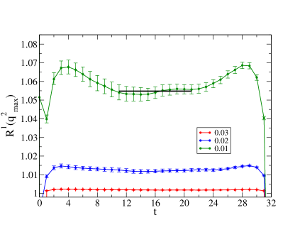
Figure 1: Ratio for $f_{0}(q_{\text{max}}^{2})$, $R^{1}(t^{\prime},t)$, as defined in Eq. (5), for three simulated light masses $am_{ud}=0.03,\,0.02,\,0.01$ for two different volumes, $16^{3}\times 32$ (left) and $24^{3}\times 64$ (right). Further simulation parameters can be found in  [11].

2.3 Investigating the momentum transfer dependence

To study the $q^{2}$ dependence of $f_{0}(q^{2})$, we construct the second ratio

$$R^{2}(t^{\prime},t;\vec{p}\,^{\prime},\vec{p})=\frac{C^{K\pi}_{4}(t^{\prime},t;\vec{p}\,^{\prime},\vec{p})C^{K}(t;\vec{0})C^{\pi}(t^{\prime}-t;\vec{0})}{C^{K\pi}_{4}(t^{\prime},t;\vec{0},\vec{0})C^{K}(t;\vec{p})C^{\pi}(t^{\prime}-t;\vec{p}\,^{\prime})}\xrightarrow[t,(t^{\prime}-t)\to\infty]{}\frac{E_{K}(\vec{p})+E_{\pi}(\vec{p}\,^{\prime})}{m_{K}+m_{\pi}}F(p^{\prime},p)\ ,$$ (7)

from which we are able to extract $f_{+}(q^{2})$ via

$$F(p^{\prime},p)=\frac{f_{+}(q^{2})}{f_{0}(q^{2}_{\text{max}})}\left(1+\frac{E_{K}(\vec{p})-E_{\pi}(\vec{p}\,^{\prime})}{E_{K}(\vec{p})+E_{\pi}(\vec{p}\,^{\prime})}\xi(q^{2})\right)\,,\ \xi(q^{2})=\frac{f_{-}(q^{2})}{f_{+}(q^{2})}\ .$$ (8)

$C^{\pi(K)}(t;\vec{p})$ in Eq. (7) is the standard pion (kaon) two point function.

Figure 2 displays a typical example of $R^{2}(t^{\prime},t;\vec{p}\,^{\prime},\vec{p})$ for bare light quark mass $am_{ud}=0.02$ and momentum transfer $|a\vec{q}|^{2}=1$, where we have set $\vec{p}\,^{\prime}=0$ and averaged over equivalent 3-momenta corresponding to the same 4-momentum transfer. The left plot shows our result from the $16^{3}\times 32$ lattice, while the right displays $24^{3}\times 64$. Note that, unlike in Section 2.2, we are now including finite spatial momentum, so disagreement between the results on the two different volumes is not an indication of finite volume effects in this case.

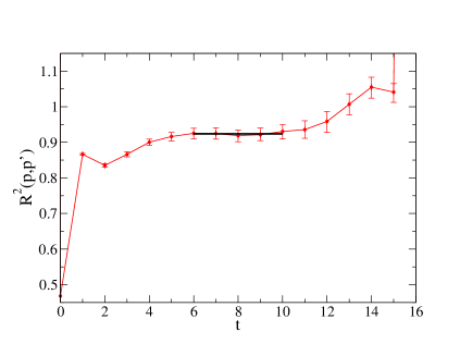
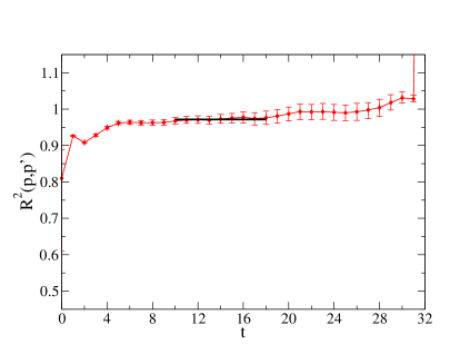
Figure 2: Ratio for $F(p,p^{\prime})$, $R^{2}(t^{\prime},t;\vec{p}\,^{\prime},\vec{p})$, as defined in Eq. (7), for bare quark mass $am_{ud}=0.02$ with momentum transfer, $|a\vec{q}|^{2}=1$ for two different volumes, $16^{3}\times 32$ (left) and $24^{3}\times 64$ (right).

Before we can extract $f_{+}(q^{2})$ from Eq. (8), we need to calculate $\xi(q^{2})=f_{-}(q^{2})/f_{+}(q^{2})$. This is achieved by constructing a third ratio:

$$R^{3}_{k}(t^{\prime},t;\vec{p}\,^{\prime},\vec{p})=\frac{C^{K\pi}_{k}(t^{\prime},t;\vec{p}\,^{\prime},\vec{p})C^{KK}_{4}(t^{\prime},t;\vec{p}\,^{\prime},\vec{p})}{C^{K\pi}_{4}(t^{\prime},t;\vec{p}\,^{\prime},\vec{p})C^{KK}_{k}(t^{\prime},t;\vec{p}\,^{\prime},\vec{p})}\quad(k=1,2,3)\ .$$ (9)

We then obtain $\xi(q^{2})$ from

$$\xi(q^{2})=\frac{-(E_{K}(\vec{p})+E_{K}(\vec{p}\,^{\prime}))(p+p^{\prime})_{k}+(E_{K}(\vec{p})+E_{\pi}(\vec{p}\,^{\prime}))(p+p^{\prime})_{k}R^{3}_{k}}{(E_{K}(\vec{p})+E_{K}(\vec{p}\,^{\prime}))(p-p^{\prime})_{k}-(E_{K}(\vec{p})-E_{\pi}(\vec{p}\,^{\prime}))(p+p^{\prime})_{k}R^{3}_{k}}\ .$$ (10)

We observe that $R^{3}_{k}(t^{\prime},t;\vec{p}\,^{\prime},\vec{p})=1$ in the $SU(3)_{\text{flavour}}$ symmetric limit, and deviates only slightly from unity at our simulation quark masses. Consequently, from Eq. (10), $\xi(q^{2})$ has a small magnitude $\mathrel{\raise 1.29167pt\hbox{$<$}\mkern-14.0mu\lower 2.58334pt\hbox{$\sim$}}0.1$ with an error typically 25%-100%.

Finally, we can double the number of available $q^{2}$ values by repeating the steps above (Eq. (7)-(10)) for the $\pi\to K$ matrix element as described in Section V of Ref. [9].

3 Results

3.1 Interpolation to $q^{2}=0$

We are now in a position to combine the results obtained above for the $f_{0}(q^{2}_{\text{max}}),\,F(p,p^{\prime})$ and $\xi(q^{2})$ to reconstruct the scalar form factor

$$f_{0}(q^{2})=f_{+}(q^{2})\left[1+\frac{q^{2}}{m_{K}^{2}-m_{\pi}^{2}}\xi(q^{2})\right]\ .$$ (11)

We present our results obtained on each volumes for $f_{0}(q^{2})$ in Fig. 3 for quark masses $am_{ud}=0.03$ (left) and $am_{ud}=0.02$ (right). In the intermediate $q^{2}$-range in both plots, we see good agreement between the results obtained on the two different volumes, indicating that finite size effects are negligible, at least for the quark masses considered here. This means that we now have results over a large range of $q^{2}$ to fit to.

We fit our data with a monopole ansatz

$$f_{0}(q^{2})=\frac{f_{0}(0)}{(1-q^{2}/M^{2})}\ ,$$ (12)

which we find to describe our data very well. This enables us to interpolate our results for $f_{0}(q^{2})$ and $f_{0}(q^{2}_{\text{max}})$ to $q^{2}=0$. Future work will involve testing several ansätze in order to obtain $f_{0}(0)$, although previous work suggests that results at the quark masses considered here are insensitive to the choice of interpolating method.

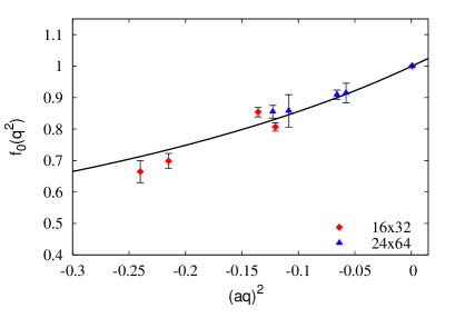
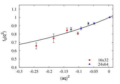
Figure 3: Scalar form factor $f_{0}(q^{2})$ for bare quark masses $am_{ud}=0.03$ (left) and 0.02 (right). Results are obtained on two volumes $V=16^{3}\times 32$ (red diamonds) and $V=24^{3}\times 64$ (blue triangles). The solid line in each plot is the result of a fit using a monopole ansatz (Eq. (12)).

3.2 Chiral Extrapolation

Now that we have obtained results for $f_{+}(0)=f_{0}(0)$ at three different quark masses, we are in a position to attempt an extrapolation to the physical pion mass. Inserting these results into the expression given in Eq. (3), together with $f_{2}$ calculated at the simulated quark masses using the ChPT formula [3, 14], we are now left with the task of chirally extrapolating $\Delta f$.

The Ademollo-Gatto Theorem implies that $\Delta f\propto(m_{s}-m_{ud})^{2}$, hence we attempt a chiral extrapolation using

$$\Delta f=a+B(m_{s}-m_{ud})^{2}\ .$$ (13)

Note that in the $SU(3)_{\text{flavour}}$ limit, $\Delta f=0$, so we expect that a fit to our data should produce $a\approx 0$.

In the left plot of Fig. 4, we show the chiral extrapolation of our results using a slightly modified version of Eq. (13) which allows the result in the chiral limit to be obtained from the intercept with the y-axis. We are encouraged by the fact that $\Delta f$ passes through zero at the $SU(3)_{\text{flavour}}$ symmetric point (denoted by the vertical dotted line), and we find in the chiral limit $\Delta f=-0.0090(11)$.

Alternatively, it has been noted that is convenient to consider an extrapolation of the ratio [5, 9]

$$R_{\Delta f}=\frac{\Delta f}{(m_{K}^{2}-m_{\pi}^{2})^{2}}=a+b(m_{K}^{2}+m_{\pi}^{2})\ .$$ (14)

Extrapolating our data using this form provides an estimate of the systematic error in the choice of chiral extrapolation (13). This obviously requires further investigation and will be reported on in a forthcoming publication. We show the extrapolation using Eq. (14) in the right plot of Fig 4 from which we extract a result at the physical meson masses (vertical dotted line). We take the difference between the results obtained from the two extrapolations (0.0011) as an estimate of the systematic error due to the chiral extrapolation.

Figure 4: The left plot shows the chiral extrapolation of $\Delta f$ using a trivial modification of Eq. (13). The vertical dotted line indicates the $SU(3)_{\text{flavour}}$ limit. The right plot is an alternative chiral extrapolation (Eq. (14))

Finally, since we only have results at one lattice spacing, we are unable to extrapolate to the continuum limit. However, lattice artefacts are formally of ${\cal O}(a^{2}\Lambda^{2}_{\text{QCD}})\approx 2.5\%$. Hence our preliminary result is

$$\Delta f=-0.0090(11)(11)(2)\Rightarrow f_{+}^{K\pi}(0)=0.9680(16)\ ,$$ (15)

where the first error is statistical, and the second and third are estimates of the systematic errors due to the chiral extrapolation and lattice aritefacts, respectively. This result agrees very well with a recent two-flavour result [9], also obtained with domain wall fermions at a similar lattice spacing $(a^{-1}\approx 1.64\,\text{GeV})$, indicating that the effects due to a dynamical strange quark are small.

Using $|V_{us}f_{+}(0)|=0.2169(9)$ from the experimental decay amplitude [15]:

$$|V_{us}|=0.2241(9)_{\text{exp}}(4)_{f_{+}(0)}$$ (16)

we find $|V_{ud}|^{2}+|V_{us}|^{2}+|V_{ub}|^{2}=1-\delta,\quad\delta=0.0015(7)$ which can be compared with result given by PDG(2006) $\delta=0.0008(11)$.

4 Summary and future work

We have presented a preliminary result for $\Delta f=f_{+}(0)-(1+f_{2})$ using $N_{f}=2+1$ dynamical domain wall fermions with three choices for the light quark masses. Our result $\Delta f=-0.0090(11)(11)(2)$ agrees very well with the $N_{f}=2$ result [9] and confirms the trend of other lattice results [5, 6, 7, 8] which prefer a negative value for $\Delta f$, in agreement with the early result of Leutwyler & Roos [3]. We performed our simulations with matched parameters on two volumes and we observe no obvious finite size effects.

This result can be improved by decreasing the error on the point at $am_{ud}=0.01$ and simulating at lighter quark masses. Additionally, this result has been obtained at a single value of the lattice spacing, so future simulations will need to be performed at least at one more lattice spacing to investigate scaling behaviour.

References

[1]
N. Cabibbo,
Phys. Rev. Lett. 10, 531 (1963);
M. Kobayashi and T. Maskawa,
Prog. Theor. Phys. 49, 652 (1973).
[2]
M. Ademollo and R. Gatto,
Phys. Rev. Lett. 13, 264 (1964).
[3]
H. Leutwyler and M. Roos,
Z. Phys. C 25, 91 (1984).
[4]
V. Cirigliano et al.,
JHEP 0504, 006 (2005)
[arXiv:hep-ph/0503108].
[5]
D. Becirevic et al.,
Nucl. Phys. B 705, 339 (2005)
[arXiv:hep-ph/0403217];
D. Becirevic et al.,
Eur. Phys. J. A 24S1, 69 (2005)
[arXiv:hep-lat/0411016].
[6]
M. Okamoto [Fermilab Lattice Collaboration],
arXiv:hep-lat/0412044.
[7]
N. Tsutsui et al. [JLQCD Collaboration],
PoS LAT2005, 357 (2006)
[arXiv:hep-lat/0510068].
[8]
C. Dawson et al.,
PoS LAT2005, 337 (2006)
[arXiv:hep-lat/0510018].
[9]
C. Dawson et al.,
arXiv:hep-ph/0607162.
[10]
Y. Iwasaki,
Nucl. Phys. B 258, 141 (1985);
Y. Iwasaki and T. Yoshie,
Phys. Lett. B 143, 449 (1984).
[11]
R. Tweedie et al., these proceedings, PoS LAT2006 096
(2006).
[12]
D. B. Kaplan,
Phys. Lett. B 288, 342 (1992)
[arXiv:hep-lat/9206013];
Y. Shamir,
Nucl. Phys. B 406, 90 (1993)
[arXiv:hep-lat/9303005].
[13]
S. Hashimoto et al.,
Phys. Rev. D 61, 014502 (2000)
[arXiv:hep-ph/9906376].
[14]
D. Becirevic, G. Martinelli and G. Villadoro,
Phys. Lett. B 633, 84 (2006)
[arXiv:hep-lat/0508013].
[15]
E. Blucher and W.J. Marciano,
“, the Cabibbo angle and CKM unitarity”, PDG,
2006.