Matrix elements and diquark correlations in quenched QCD with overlap fermions.

Abstract:

We present results for $B_{K}$ and selected matrix elements for beyond the standard model interactions obtained in quenched QCD with overlap fermions. We also illustrate results on baryon wave-functions and diquark correlations within baryons in the Coulomb and Landau gauge.

1 Introduction

Over the last few years we have performed a study of quenched QCD with overlap quarks. We generated 100 configurations of size $18^{3}\times 64$ at $\beta=6$ and 100 configurations of size $14^{3}\times 48$ at $\beta=5.85$, with Wilson gauge action and separated from each other by 10,000 Metropolis steps. The corresponding lattice spacings, from the Sommer scale, are $a^{-1}=2.12{\rm GeV}$ and $a^{-1}=1.61{\rm GeV}$. These configurations were transformed to the Landau gauge, and overlap quark propagators were calculated for a single point source and all 12 color-spin combinations with $\rho=1.4$, $am_{q}=0.03,0.04,0.06,0.08,0.1,0.25,0.5,0.75$ at $\beta=6$, and $\rho=1.6$, $am_{q}=0.03,0.04,0.053,0.08,0.106,$ $0.132,0.33,0.66,0.99$ at $\beta=5.85$. (We recall that the overlap Dirac operator for a quark of mass $m$ is given by $[1-(am)/(2\rho)]D+m$, where $D=(\rho/a)(1+\gamma_{5}H(\rho)/\sqrt{H(\rho)^{2}})$ and $H(\rho)$ stands for the Hermitian Wilson-Dirac operator with mass $-\rho/a$.) A Zolotarev approximation to the inverse square root was used for the first 55 configurations at $\beta=6$, then a Chebyshev approximation of degree $100\sim 500$, after Ritz projection of the 12 ($18^{3}\times 64$ lattice) or 40 ($14^{3}\times 48$ lattice) lowest eigenvectors of $H^{2}$. The convergence criterion was $|x^{-1/2}-\sum T_{n}(x)|<10^{-8}$, $|D^{\dagger}D\psi-\chi|^{2}<10^{-7}$. The use of propagators with a point source, as opposed to extended or wall sources, was dictated by our desire to calculate matrix elements and renormalization factors, and by the limitation of the computational resources at our disposal. Results for light hadron spectroscopy were presented at the Lattice 2005 Symposium [1] and in Ref. [2]. We refer the reader to [2] for details of our calculations and for references to other studies of lattice QCD with overlap quarks on large lattices. We present here results we recently obtained on $\Delta S=2$ matrix elements and on baryon wave-functions and diquark correlations inside baryons.

2 $\Delta S=2$ matrix elements

We evaluated matrix elements of the operators $O_{1}=[\bar{s}^{a}\gamma_{\mu}(1-\gamma_{5})d^{a}][\bar{s}^{b}\gamma^{\mu}(1-\gamma_{5})d^{b}],O_{2}=[\bar{s}^{a}(1-\gamma_{5})d^{a}][\bar{s}^{b}(1-\gamma_{5})d^{b}],O_{3}=[\bar{s}^{a}(1-\gamma_{5})d^{b}][\bar{s}^{b}(1-\gamma_{5})d^{a}],O_{4}=[\bar{s}^{a}(1-\gamma_{5})d^{a}][\bar{s}^{b}(1+\gamma_{5})d^{b}]$ and $O_{5}=[\bar{s}^{a}(1-\gamma_{5})d^{b}][\bar{s}^{b}(1+\gamma_{5})d^{a}]$ which are needed to study neutral kaon mixing in the standard model (SM) and beyond (BSM). An extensive description of our work and results has been presented in [3]. Here we we only outline the main features of our analysis. We would like to direct the reader to [3] for a detailed bibliography of other relevant investigations.

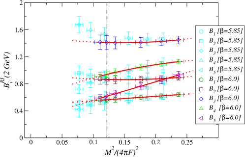
Figure 1: Mass-dependence, in terms of the variable $M^{2}/(4\pi F)^{2}$, of the $B$-parameters $B_{i}$, $i=1,\cdots,5$, in the RI/MOM scheme at $2$ GeV. The solid curves are the results of the fits described in the text, and are plotted in the fit region. The fits are used to interpolate the results to the kaon point $M^{2}/(4\pi F)^{2}=M_{K}^{2}/(4\pi F_{K})^{2}$, shown as a vertical dotted line. The dashed curves are an extension of the fit curves outside the fit range.

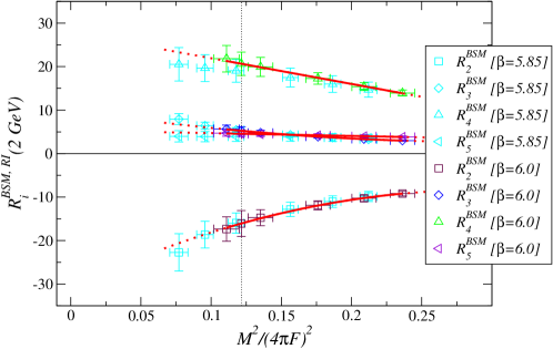
Figure 2: Same as Figure 1, but for the BSM ratios $R_{i}^{\mathrm{BSM}}$, $i=2,\cdots,5$.

We used the quark propagators to calculate

$${\cal B}^{1}_{PP}(x_{0},y_{0}) = \frac{\sum_{\vec{x},\vec{y}}{\langle P(x)O_{1}(0)P(y)\rangle}}{\frac{8}{3}\sum_{\vec{x},\vec{y}}{\langle P(x)\bar{A}_{0}(0)\rangle\langle\bar{A}_{0}(0)P(y)\rangle}}\stackrel{{\scriptstyle a\ll x_{0}\ll T/2\ll y_{0}\ll T}}{{\longrightarrow}}B_{1}$$ (1)

$${\cal B}^{i}_{PP}(x_{0},y_{0}) = \frac{\sum_{\vec{x},\vec{y}}{\langle P(x)O_{i}(0)P(y)\rangle}}{N_{i}\sum_{\vec{x},\vec{y}}{\langle P(x)\bar{P}(0)\rangle\langle\bar{P}(0)P(y)\rangle}}\stackrel{{\scriptstyle a\ll x_{0}\ll T/2\ll y_{0}\ll T}}{{\longrightarrow}}B_{i}$$ (2)

for $i{=}2\cdots 5$ with $N_{i}={\frac{5}{3},-\frac{1}{3},-2,-\frac{2}{3}}$, and fit to a constant in the symmetric time intervals given by: $12\leq x_{0}/a\leq 19$ and $45\leq y_{0}/a\leq 52$ for $i{=}1\cdots 5$, at $\beta=6.0$; $10\leq x_{0}/a\leq 12$ and $36\leq y_{0}/a\leq 38$ for $i{=}1$ and $10\leq x_{0}/a\leq 14$ and $34\leq y_{0}/a\leq 38$ for $i{=}2\cdots 5$, at $\beta=5.85$.

The bare values obtained for the parameters $B_{i}$ must be renormalized to relate them to physical observables. We used a non-perturbative renormalization technique based on the RI/MOM methods of [4]. Our results for the $B$-parameters are shown in Figure 1, where the polynomial interpolations to the kaon point are displayed. From these $B$-parameters, we also reconstruct the matrix elements themselves. In Figure 2, we show the polynomial interpolations to the kaon point of the ratios:

$$R_{i}^{\mathrm{BSM}}(\mu,M^{2})\equiv\left[\frac{F_{K}^{2}}{M_{K}^{2}}\right]_{expt}\left[\frac{M^{2}}{F^{2}}\frac{\langle\bar{P}^{0}|O_{i}(\mu)|P^{0}\rangle}{\langle\bar{P}^{0}|O_{1}(\mu)|P^{0}\rangle}\right]_{lat},$$ (3)

for $i=2,\cdots,5$, where $M$ and $F$ are the mass and “decay constant” of the lattice kaon which we denote by $P^{0}$ to indicate that the mass of the strange and down quarks that compose it can differ from their physical values. The ratios $R_{i}^{\mathrm{BSM}}(\mu,M_{K}^{2})$ measure directly the ratio of BSM to SM matrix elements and, as such, can be used in expressions for $\Delta M_{K}$ and $\epsilon$ beyond the SM, in which the SM contribution is factored out.

Our main conclusion is that the non-SM, $\Delta S=2$ matrix elements are significantly larger than found in the only other dedicated lattice study of these amplitudes [5]. In tracing the source of this difference, we found that we already disagree on the much simpler matrix element of the pseudoscalar density between a kaon state and the vacuum, which is the building block for the vacuum saturation values of the BSM $\Delta S=2$ amplitudes. Through the axial Ward identity, the matrix element of the pseudoscalar density is related to the sum of the strange and down quark masses, which we find to be roughly 30% smaller than the value obtained in [6], with the same tree-level improved Wilson fermion action and gauge configurations as used in [5]. Since our result for this sum of masses is in agreement with the continuum limit, benchmark result of [7], we are convinced that the stronger enhancement of non-SM $\Delta S=2$ matrix elements that we observe is correct. For details concerning this issue as well as our other results, we refer the reader to [3].

3 Baryon wave-functions and diquark correlations

We study the correlation of quarks inside baryons by evaluating baryon Green functions where the quarks, which without loss of generality we take to be $u,d$ and $s$, are found at different spatial locations at the sink:

$$G(\vec{r}_{1},\vec{r}_{2},\vec{r}_{3},t)=\langle u(\vec{r}_{1},t)d(\vec{r}_{2},t)s(\vec{r}_{3},t)\;\bar{u}(0)\bar{d}(0)\bar{s}(0)\rangle$$ (4)

The color indices, which like the spin indices are left implicit, are combined in a color singlet. The use of gauge fixing allows us to consider separated quarks without the need to introduce gauge transport factors. For this investigation we also converted the gauge background field from the Landau gauge to the Coulomb gauge, and we will report below results in both gauges, which however are rather similar. In order to project over states of zero momentum, we sum over a translational degree of freedom, evaluating a reduced wave function

$$\tilde{G}(\vec{r},\vec{r}^{\prime},t)=\sum_{\vec{r}_{3}}\langle u(\vec{r}_{3}+\vec{r},t)d(\vec{r}_{3}+\vec{r}^{\prime},t)s(\vec{r}_{3},t)\;\bar{u}(0)\bar{d}(0)\bar{s}(0)\rangle$$ (5)

(The sums in 5 involve a very large number of terms and the use of a fast Fourier transform and the convolution theorem is crucial to carry them out in manageable computer time).

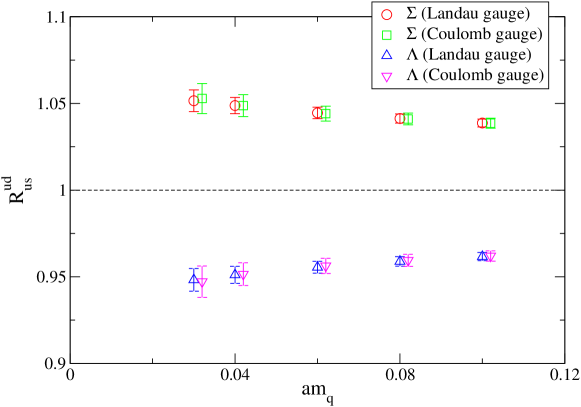
Figure 3: Ratio of mean $u-d$ separation to mean $u-s$ separation as function of quark mass for the two $u,d$ diquark configurations. Data with $\beta=6$ and $t=10a$.

The spin indices are combined in an appropriate spin wave-function at the source and sink. Of particular interest is comparing the spin configurations where, in the spin $1/2^{+}$ octet, the $u$ and $d$ quarks are combined, $\Lambda$-like , in a spin and isospin singlet state, the so-called good diquark combination, versus those where $u$ and $d$ are, $\Sigma$-like, in a spin and isospin triplet state. In Figure 3 we show the ratio of the mean separations between $u,d$ and $u,s$ quarks in the two spin states. The results give support to the notion that quarks inside a baryon tend to correlate in a “good” diquark state.

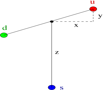
Figure 4: The geometry used for visualizing the wave-function of the quarks inside a baryon.

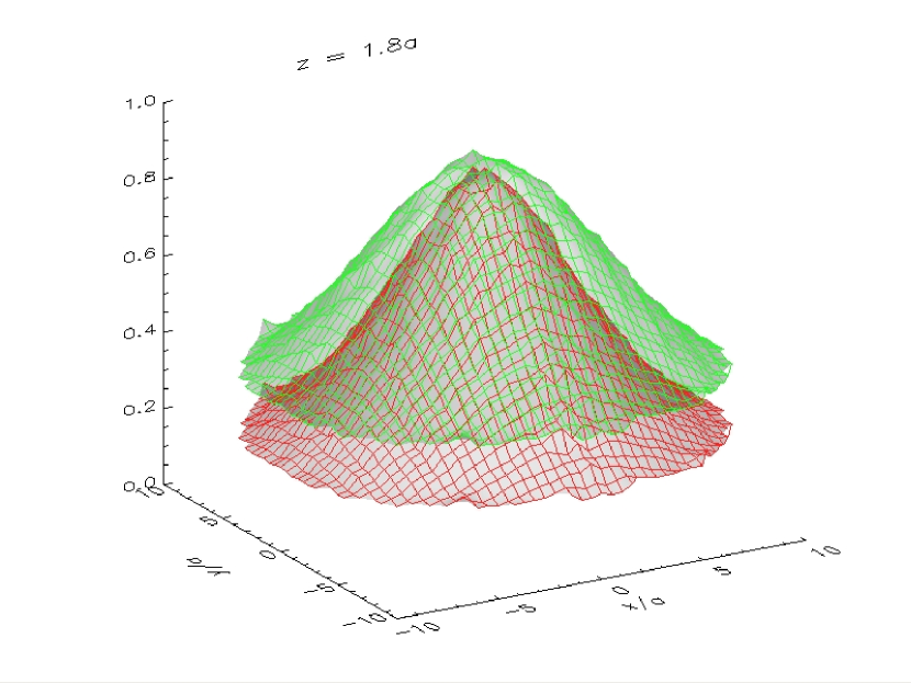
Figure 5: The wave-function of the $u$ and $d$ quarks, in the Coulomb gauge, in a spin and isospin singlet state (good diquark), given by the narrower bell-shaped surface (red with color), against the wave-function of the two quarks in a spin and isospin triplet state, given by the broader curve (green with color), for a separation $z=1.8a$ between the $s$ quark and the mid-point of the $u,d$ pair.

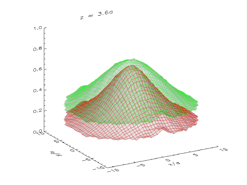
Figure 6: Same as in Figure 5, but for $z=3.6a$.

It is interesting to visualize the correlation among the quarks inside the baryon, i.e. the function $\tilde{G}(\vec{r},\vec{r}^{\prime},t)$ which we can loosely consider as the wave-function of the three quarks. The problem is, of course, that, at fixed $t$, $\tilde{G}$ is a function of the two vectors $\vec{r},\vec{r}^{\prime}$, i.e. of six variables. The representation of $\tilde{G}$ can be simplified somewhat by assuming rotational invariance, i.e. lack of major spin orbit correlation. We have verified that this assumption is satisfied within the statistical accuracy of our calculations. (Indeed the actual magnitude of spin-orbit correlations could be evaluated by our technique, given sufficient statistical precision.) This leaves $\tilde{G}$ a function only of the shape of the triangle subtended by the two vectors $\vec{r},\vec{r}^{\prime}$. This is still a function of three variables, but, to provide a meaningful visualization, we can fix one of these and represent the wave-function as a function of the other two. Thus, for a generic triangle formed by the locations of the $s,u$ and $d$ quarks, we introduce coordinates $x,y,z$ as illustrated in Figure 4, and then represent $\tilde{G}$ as a function in the $x,y$ plane at fixed $z$. Our results, with $\beta=6$, $am_{q}=0.03$ and $t=10a$, are illustrated in Figures 5 and 6. They show again that the $u$ and $d$ quarks tend to correlate in the good diquark configuration.

A detailed, expanded version of the results presented in this section is in preparation and will form the subject of a forthcoming paper. An earlier study of quark wave-functions with some similarity to ours can be found in Ref. [8]. We are not aware of other investigations studying the same type of correlation functions.

4 Conclusions

Our results corroborate the fact that the overlap discretization, at least insofar as valence quarks are concerned, can be used in large scale simulations, and, because of its very good symmetry properties, represents a choice method for QCD numerical calculations.

They also provide some novel matrix element values and evidence for strong diquark correlation in a flavor $\bar{3}$, spin-singlet state.

- [1] R. Babich, F. Berruto, N. Garron, C. Hoelbling, J. Howard, L. Lellouch, C. Rebbi, and N. Shoresh PoS LAT2005 (2006) 043, hep-lat/0509182.
- [2] R. Babich, F. Berruto, N. Garron, C. Hoelbling, J. Howard, L. Lellouch, C. Rebbi, and N. Shoresh JHEP 01 (2006) 086, hep-lat/0509027.
- [3] R. Babich, N. Garron, C. Hoelbling, J. Howard, L. Lellouch, and C. Rebbi hep-lat/0605016. to be published in Phys. Rev. D.
- [4] G. Martinelli, C. Pittori, C. T. Sachrajda, M. Testa, and A. Vladikas Nucl. Phys. B445 (1995) 81–108, hep-lat/9411010.
- [5] A. Donini, V. Gimenez, L. Giusti, and G. Martinelli Phys. Lett. B470 (1999) 233–242, hep-lat/9910017.
- [6] V. Gimenez, L. Giusti, F. Rapuano, and M. Talevi Nucl. Phys. B540 (1999) 472–490, hep-lat/9801028.
- [7] ALPHA Collaboration, J. Garden, J. Heitger, R. Sommer, and H. Wittig Nucl. Phys. B571 (2000) 237–256, hep-lat/9906013.
- [8] M. W. Hecht et al. Phys. Rev. D47 (1993) 285–294, hep-lat/9208005.