Signatures of $S$-wave bound-state formation in finite volume

Abstract

We discuss formation of an $S$-wave bound state in finite volume on the basis of Lüscher’s phase-shift formula. It is found that although a bound-state pole condition is fulfilled only in the infinite volume limit, its modification by the finite size corrections is exponentially suppressed by the spatial extent $L$ in a finite box $L^{3}$. We also confirm that the appearance of the $S$-wave bound state is accompanied by an abrupt sign change of the $S$-wave scattering length even in finite volume through numerical simulations. This distinctive behavior may help us to distinguish the loosely bound state from the lowest energy level of the scattering state in finite volume simulations.

I Introduction

In the past few years, several new hadronic resonances have been discovered in various experiments Klempt:2004yz . However, some of the states have unusual properties, which are not well understood from the viewpoint of the conventional quark-antiquark or three-quark states. It is a great challenge for lattice QCD to answer the question, whether those states are really exotic hadron states.

We are especially interested in some candidates of hadronic molecular state: the $\Lambda$(1405) resonance as an $\overline{K}N$ bound state, the $f_{0}(980)$ and $a_{0}(980)$ resonances as $S$-wave bound states of $K\overline{K}$, the $X(3872)$ resonance as a weakly bound state of $D\overline{D}^{*}$, the $D_{s0}(2317)$ and $D_{s1}(2460)$ resonances as $D^{(*)}K$ bound states and so on Rosner:2006vc . Such states lie near and below their respective thresholds so that one can view them as “loosely bound states” of two hadrons like a deuteron.

In the infinite volume, the loosely (near-threshold) bound state is well defined since there is no continuum state below threshold. However, in a finite box on the lattice, all states have discrete energies. Even worse, the lowest energy level of the elastic scattering state appears below threshold in the case if an interaction is attractive between two particles Luscher:1985dn ; Luscher:1990ux . Therefore, there is an ambiguity to distinguish between the loosely bound state and the lowest scattering state in finite volume in this sense.

Signatures of bound-state formation in finite volume are of main interest in this paper. We may begin with a naive question: what is the legitimate definition of the loosely bound state in the quantum mechanics? In the scattering theory Newton:1982qc , poles of the $S$-matrix or the scattering amplitude correspond to bound states. It is also known that the appearance of the $S$-wave bound state is accompanied by an abrupt sign change of the $S$-wave scattering length Newton:1982qc . It is interpreted that formation of one bound-state raises the phase shift at threshold by $\pi$. This particular feature is generalized as Levinson’s theorem Newton:1982qc . Thus, it is interesting to consider how the formation condition of bound states is implemented in Lüscher’s finite size method, which is proposed as a general method for computing low-energy scattering phases of two particles in finite volume Luscher:1985dn ; Luscher:1990ux .

In this paper, we discuss bound-state formation on the basis of the phase-shift formula in this method and then present our proposal for numerical simulations to distinguish the loosely bound state from the lowest scattering state in finite volume. To exhibit the validity and efficiency of our proposal, we perform numerical studies of the positronium spectroscopy in compact scalar QED model. In the Higgs phase of $U(1)$ gauge dynamics, the photon is massive and then massive photons give rise to the short-ranged interparticle force between an electron and a positron exponentially damped. In this model, we can control positronium formation in variation with the strength of the interparticle force and then explore distinctive signatures of the bound-state formation in finite volume.

The organization of our paper is as follows. In Sec. II, we first give a brief review of Lüscher’s finite size method Luscher:1985dn ; Luscher:1990ux and discuss bound-state formation on the basis of the phase-shift formula in this method. Sec. III gives details of our utilized model, compact scalar QED, and its Monte Carlo simulations. Secs. IV and  V are devoted to discuss our numerical results in the ${}^{1}S_{0}$ and ${}^{3}S_{1}$ channels of electron-positron system, respectively. Finally, in Sec. VI, we summarize the present work and give our concluding remark. In addition, there are two appendices. In Appendices A, the sensitivity of mass spectra to choice of spatial boundary condition is discussed. We also demonstrate a specific volume dependence of the spectral amplitude for either the bound state or the lowest scattering state in Appendix B.

II Methodology

II.1 Lüscher’s finite size method for scattering phase shift

Let us briefly review Lüscher’s finite size method Luscher:1985dn ; Luscher:1990ux . So far, several hadron scattering lengths, e.g. $\pi$-$\pi$, $\pi$-$K$, $\pi$-$N$, $K$-$N$, $N$-$N$ and $J/\psi$-hadron, have been successfully calculated by using this method Guagnelli:1990jb ; Sharpe:1992pp ; Gupta:1993rn ; Fukugita:1994ve ; Aoki:2002in ; Aoki:2002ny ; Yamazaki:2004qb ; Aoki:2005uf ; Beane:2005rj ; Beane:2006mx ; Beane:2006gj ; Liu:2001ss ; Miao:2004gy ; Meng:2003gm ; Hasenfratz:2004qk ; Yokokawa:2006td .

The total energy of two-particle states in the center-of-mass frame is given by

$$E_{AB}(p)=\sqrt{m_{A}^{2}+p^{2}}+\sqrt{m_{B}^{2}+p^{2}},$$ (1)

where $p$ is the relative momentum of two particles. In a finite box $L^{3}$ on the lattice, all momenta are quantized and can be labeled by an integer $n$ as ${\bar{p}}_{n}$, which represents the $(n+1)$-th lowest momentum. Therefore, all two-particle states have only discrete energies.

We introduce the scaled momentum as $q=L{\bar{p}}_{n}/2\pi$ with the spatial extent $L$ for periodic boundary condition. Although the value of $q^{2}$ takes an integer value in the non-interacting case, $q^{2}$ is no longer the integer due to the presence of the two-particle interaction. This particular feature can be observed through an energy shift relative to the energy of the non-interacting two particles,

$$\Delta E=E_{AB}({\bar{p}}_{n})-E_{AB}(p_{n}),$$ (2)

where the energy of non-interacting two-particle states $E_{AB}(p_{n})$ can be evaluated with the quantized momentum $p_{n}$ in the free case as $p_{n}=2\pi\sqrt{n}/L$ with an integer $n$.

It has been shown by Lüscher that this energy shift in a finite box with a spatial size $L$ can be translated into the $S$-wave phase shift $\delta_{0}$ through the relation Luscher:1985dn ; Luscher:1990ux :

$$\tan\delta_{0}({\bar{p}}_{n})=\frac{\pi^{3/2}\sqrt{q^{2}}}{{\cal Z}_{00}(1,q^{2})}\;\;\;\;{\rm at}\;\;q=L{\bar{p}}_{n}/2\pi,$$ (3)

where the function ${\cal Z}_{00}(s,q^{2})$ is an analytic continuation of the generalized zeta function, ${\cal Z}_{00}(s,q^{2})\equiv\frac{1}{\sqrt{4\pi}}\sum_{{\bf n}\in Z^{3}}({\bf n}^{2}-q^{2})^{-s}$, from the region $s>3/2$ to $s=1$. The $S$-wave scattering length is defined through $a_{0}=\lim_{p\rightarrow 0}\tan\delta_{0}(p)/p$.

If the $S$-wave scattering length $a_{0}$ is sufficiently smaller than the spatial size $L$, one can make a Taylor expansion of the phase-shift formula (3) around $q^{2}=0$, and then obtain the asymptotic solution of Eq. (3). Under the condition $p^{2}\ll m_{A}^{2}$ and $m_{B}^{2}$, the solution is given by

$$\Delta E_{q^{2}=0}\approx-\frac{2\pi a_{0}}{\mu L^{3}}\left[1+c_{1}\frac{a_{0}}{L}+c_{2}\left(\frac{a_{0}}{L}\right)^{2}\right]+{\cal O}(L^{-6}),$$ (4)

which corresponds to the energy shift of the lowest ($n=0$) scattering state. The coefficients are $c_{1}=-2.837297$ and $c_{2}=6.375183$ Luscher:1985dn ; Luscher:1990ux . The reduced mass of two particles $\mu$ is given by $\mu=m_{A}\cdot m_{B}/(m_{A}+m_{B})$. An important message is received from Eq. (4). The lowest energy level of the elastic scattering state appears below threshold on the lattice if an interaction is weakly attractive ($a_{0}>0$) between two particles. This point makes it difficult to distinguish between near-threshold bound states and scattering states on the lattice.

Here, it is worth noting that the large $L$ expansion formula (4) up to $O(L^{-4})$ gives no real solution of $a_{0}$ for the case $\Delta E<-\frac{\pi}{2|c_{1}|\mu L^{2}}$ Yokokawa:2006td , while Eq. (4) with an expansion up to $O(L^{-4})$ and that up to $O(L^{-5})$ always possesses a real and negative solution of $a_{0}$ for $\Delta E>0$. A lower bound $\Delta E\geq-\frac{\pi}{2|c_{1}|\mu L^{2}}$ may be crucial to identify the observed state below threshold as the lowest energy level of the elastic scattering state.

For the second lowest ($n=1$) scattering state, we also obtain a different asymptotic solution of Eq. (3), which is given by a Taylor expansion of the phase-shift formula (3) around $q^{2}=1$ as

$$\Delta E_{q^{2}=1}\approx-\frac{6\tan\delta_{0}({\bar{p}}_{1})}{\mu L^{2}}\left[1+c_{1}^{\prime}\tan\delta_{0}({\bar{p}}_{1})+c_{2}^{\prime}\tan^{2}\delta_{0}({\bar{p}}_{1})\right]+{\cal O}(L^{-6}),$$ (5)

where $c_{1}^{\prime}=-0.061367$ and $c_{2}^{\prime}=-0.354156$. Although the sign of $\tan\delta_{0}$ is not uniquely related to the sign of the energy shift, the resulting energy shift $\Delta E$ becomes positive (negative) for the weak repulsive (attractive) interaction case ($|\delta_{0}|\mathrel{\hbox to0.0pt{\raise 2.20013pt\hbox{$<$}\hss}{\lower 2.20013pt\hbox{$\sim$}}}3\pi/5$). Subsequently, one can derive the asymptotic solutions for the higher energy levels of the scattering state around $q^{2}=\nu\geq 2$ where $\nu={\bf n}^{2}$ for integer 3-dim vectors ${\bf n}\in Z^{3}$. For those asymptotic solutions, the corresponding relative momentum ${\bar{p}}_{n}$, which we will hereafter abbreviate as $p$, should vanish as $1/L$ with increasing $L$.

II.2 Bound-state formation in Lüscher’s formula

In quantum scattering theory, the formation condition of bound states is implemented as a pole in the $S$-matrix or scattering amplitude. Therefore, an important question naturally arises as to how bound-state formation is studied through Lüscher’s phase-shift formula (3) .

Intuitively, the pole condition of the $S$-matrix: $S={\rm e}^{2i\delta_{0}(p)}=\frac{\cot\delta_{0}(p)+i}{\cot\delta_{0}(p)-i}$ is expressed as

$$\cot\delta_{0}(p)=i,$$ (6)

which is satisfied at $p^{2}=-\gamma^{2}$ where positive real $\gamma$ represents the binding momentum. In fact, as we will discuss in the following, such a condition is fulfilled only in the infinite volume. However the finite-volume corrections on this pole condition are exponentially suppressed by the size of spatial extent $L$.

For negative $q^{2}$, an exponentially convergent expression of the zeta function ${\cal Z}_{00}(s,q^{2})$ has been derived in Ref. Elizalde:1997jv . For $s=1$, it is given by

$${\cal Z}_{00}(1,q^{2})=-\pi^{3/2}\sqrt{-q^{2}}+\sum_{{\bf n}\in{\bf Z^{3}}}{}^{\prime}\frac{\pi^{1/2}}{2\sqrt{\bf n^{2}}}e^{-2\pi\sqrt{-q^{2}{\bf n^{2}}}},$$ (7)

where $\sum^{\prime}_{{\bf n}\in Z^{3}}$ means the summation without ${\bf n}=(0,0,0)$. We now insert Eq. (7) into Eq. (3) and then obtain the following formula, which is mathematically equivalent to Eq. (3) for negative $q^{2}$:

$$\cot\delta_{0}(p)=i+\frac{1}{2\pi i}\sum_{{\bf n}\in{Z^{3}}}{}^{\prime}\frac{1}{\sqrt{-q^{2}{\bf n}^{2}}}e^{-2\pi\sqrt{-q^{2}{\bf n}^{2}}}.$$ (8)

The second term in the r. h. s. of Eq. (8) vanishes in the limit of $q^{2}\rightarrow-\infty$. It clearly indicates that negative infinite $q^{2}$ is responsible for the bound-state formation. Therefore, in this limit, the relative momentum squared $p^{2}$ approaches $-\gamma^{2}$, which must be non-zero. Meanwhile, the negative infinite $q^{2}$ turns out to be the infinite volume limit. This representation shows that although the pole condition is fulfilled in the infinite volume, its modification in finite volume is described by correction terms, which are exponentially suppressed by the size of spatial extent $L\propto q$.

Although it was pointed out how the bound-state pole condition could be implemented in his phase-shift formula in the original paper Luscher:1990ux , another type of large $L$ expansion formula around $q^{2}=-\infty$ has been explicitly derived in Ref. Beane:2003da .

$$\Delta E_{q^{2}=-\infty}=-\frac{\gamma^{2}}{2\mu}\left[1+\frac{12}{\gamma L}\frac{1}{1-2\gamma(p\cot\delta_{0})^{\prime}}e^{-\gamma L}+{\cal O}(e^{-\sqrt{2}\gamma L})+{\cal O}(\gamma^{2}/\mu^{2})\right],$$ (9)

where $(p\cot\delta_{0})^{\prime}=\frac{d}{dp^{2}}(p\cot\delta_{0})|_{p^{2}=-\gamma^{2}}$. An $L$-independent term $-\frac{\gamma^{2}}{2\mu}$ corresponds to the binding energy in the infinite volume limit. We can learn from Eq. (9) that “loosely bound states” are supposed to receive larger finite volume corrections than those of “tightly bound states” since the expansion parameter is scaled by the binding momentum $\gamma$. Furthermore, it can be expected that the bound state of two or more particles has a kinematical nature similar to a single particle if the spatial size $L$ is much larger than the size of its compositeness, which may be characterized by the inverse of the binding momentum.

II.3 Novel view from Levinson’s theorem

At last, a crucial question arises: once the $S$-wave bound states are formed, what is the fate of the lowest $S$-wave scattering state? The answer to this question might provide a hint to resolve our main issue of how to distinguish between “loosely bound states” and scattering states. A naive expectation from Levinson’s theorem in quantum mechanics is that the energy shift relative to a threshold turns out to be opposite in comparison to the case where there is no bound state. Levinson’s theorem relates the elastic scattering phase shift $\delta_{l}$ for the $l$-th partial wave at zero relative momentum to the total number of bound states ($N_{l}$) in a beautiful relation :

$$\delta_{l}(0)=N_{l}\pi.$$ (10)

Therefore, if an $S$-wave bound state is formed in a given channel, the $S$-wave scattering phase shift should always be positive at low energies. This positiveness of the scattering phase shift is consistent with a consequence of the attractive interaction. Conversely, the $S$-wave scattering length may become negative ($a_{0}<0$) as schematically depicted in Fig 1. Consequently, according to Eq. (4) , possible negativeness of the scattering length gives rise to a positive energy-shift of the lowest scattering state relative to the threshold energy. In other words, the lowest ($n=0$) scattering state is pulled up into the region above threshold. Therefore, the spectra of the scattering states quite resembles the one in the case of the repulsive interaction. If it were true, we can observe a significant difference in spectra above the threshold between the two systems: one has at least one bound state (bound system) and the other has no bound state (unbound system).

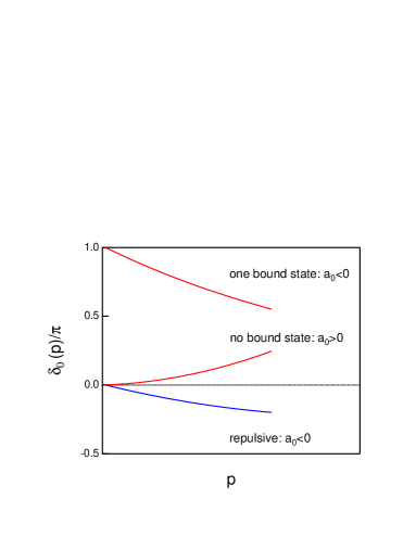
Figure 1: A schematic figure for the scattering phase shift as a function of the relative momentum of two-particle.

III Setup of numerical simulations

III.1 Compact Scalar QED

To explore signatures of bound-state formation on the lattice, we consider a bound state (positronium) between an electron and a positron in the compact QED with scalar matter:

$$S_{\rm SQED}[U,\Phi,\Psi]=S_{\rm AH}[U,\Phi]+\sum_{\rm sites}\overline{\Psi}_{x}D_{\rm W}[U]_{x,y}\Psi_{y},$$ (11)

which is the compact $U(1)$ gauge theory coupled to both scalar matter (Higgs) fields $\Phi$ and fermion (electron) fields $\Psi$. The action of “$U(1)$ gauge + Higgs” part is described by the compact $U(1)$-Higgs model:

$$S_{\rm AH}[U,\Phi]=\beta\sum_{\rm plaq.}\left[1-\Re\{U_{x,\mu\nu}\}\right]-h\sum_{\rm link}\Re\{\Phi^{\ast}_{x}U_{x,\mu}\Phi_{x+{\mu}}\},$$ (12)

where $\beta=1/e^{2}$ and the constraint $|\Phi_{x}|=1$ is imposed. In tree level, the vacuum expectation value of the Higgs field and the photon mass are interpreted as $\langle\phi_{\rm higgs}\rangle\sim a^{-1}\sqrt{h}$ and $M_{\rm ph}\sim a^{-1}\sqrt{h/\beta}$ respectively Fradkin:1978dv . In the Higgs phase, the Coulomb potential should be screened by the massive photon fields:

$$V(r)\simeq\frac{e^{2}}{4\pi}\frac{e^{-M_{\rm ph}r}}{r}.$$ (13)

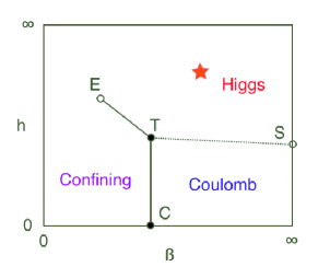
Figure 2: Schematic phase diagram of the compact $U(1)$-Higgs model in the fixed modulus case. A star mark represents our simulation point as $(\beta,h)=(2.0,\;0.6)$.

The phase structure of the $U(1)$-Higgs model has been well studied on the lattice. Fig.2 shows a schematic phase diagram of the compact $U(1)$-Higgs model. There are three phases: the confinement phase, the Coulomb phase and the Higgs phase. The open symbols and filled symbols represent the second-order phase transition points (E: the end point $\{\beta,h\}=\{0.8485(8),0.5260(9)\}$ Alonso:1992zg and S: the 4-dim XY model phase transition) and the first-order phase transition points (T: the triple point $\{\beta,h\}\sim\{1,0.36\}$ and C: the pure compact $U(1)$ phase transition $\beta_{c}\simeq 1.01$) respectively. Lines ET and TC represent the first order line. A dotted line TS corresponds to the Coulomb-Higgs transition, of which the order is somewhat controversial in the literature because of large finite size effects.

III.2 Monte Carlo simulation

In this numerical study, we treat the fermion fields in the quenched approximation. Therefore, for update of gauge links and Higgs fields, we simply adopt the Metropolis algorithm. First, the acceptance is adjusted to about 30%. Then we use 16 hits at each link and Higgs field update.

Our purpose is to study the $S$-wave bound state and scattering states through Lüscher’s finite size method, which is only applied to the short-ranged interaction case. Thus, we fix $\beta=2.0$ and $h=0.6$ in Eq.(12) to simulate the Higgs phase of $U(1)$ gauge dynamics, where massive photons give rise to the short-ranged interparticle force between an electron and a positron. We generate $U(1)$ gauge configurations with a parameter set, $(\beta,h)=(2.0,0.6)$, on $L^{3}\times 32$ lattices with several spatial sizes, $L=12,16,20,24,28$ and 32. Statistics for each volume calculation are summarized in Table 1.

Table 1: Simulation statistics

Spatial size ($L$)	12	16	20	24	28	32
# of conf.	960	1920	1280	720	720	480

Once the parameters of the compact $U(1)$-Higgs action, $(\beta,h)$, are fixed, the strength of an interparticle force between electrons should be frozen on given gauge configurations. However, if we consider the fictitious $Q$-charged electron, the interparticle force can be controlled by this charge $Q$ since the interparticle force is proportional to (charge $Q)^{2}$. Within the quenched approximation, this trick of the $Q$-charged electron is easily implemented by replacing $U(1)$ link fields as

$$U_{x,\mu}\longrightarrow U^{Q}_{x,\mu}=\Pi_{i=1}^{Q}U_{x,\mu}$$ (14)

into the Wilson-Dirac matrix:

$$D_{\rm W}[U^{Q}]_{x,y}=\delta_{x,y}-\kappa\sum_{\mu}\left[(1-\gamma_{\mu})U^{Q}_{x,\mu}\delta_{x+\mu,y}+(1+\gamma_{\mu})U_{x-\mu,\mu}^{Q\dagger}\delta_{x-\mu,y}\right],$$ (15)

where $\kappa$ is the hopping parameter.

For the matrix inversion, we use the BiCGStab algorithm Frommer:1994vn and adopt the convergence condition $|r|<10^{-15}$ for the residues. We calculate the electron propagators $\langle 0|\Psi(x)\overline{\Psi}(y)|0\rangle=D^{-1}_{\rm W}[U^{Q}]_{x,y}$ with both periodic and anti-periodic boundary conditions in the temporal direction. Then, we adopt the averaged propagator over the boundary conditions. This procedure provides an electron propagator with $2T$-periodicity Sasaki:2001nf ; Sasaki:2005ug .

III.3 Spectrum of single electron

To evaluate a threshold energy of the electron-positron ($e^{-}e^{+}$) system, it is necessary to calculate the electron mass nonperturbatively by the following two-point correlator,

$$G_{e}(t;{\bf p}_{n})=\frac{1}{L^{6}}\sum_{{\bf x},{\bf y}}{\rm Tr}\{{\cal P}_{+}\langle 0|\Psi({\bf x},t)\overline{\Psi}({\bf y},0)|0\rangle e^{i{\bf p}_{n}\cdot({\bf x}-{\bf y})}\},$$ (16)

where ${\cal P}_{+}=\frac{1+\gamma_{4}}{2}$ and ${\bf p}_{n}=\frac{2\pi}{L}{\bf n}$ with ${\bf n}\in Z^{3}$ for the periodic boundary condition in spatial directions. Here, we have set the lattice spacing to unity ($a=1$). This electron two-point correlator is gauge-variant, so gauge fixing is required. We fix to the Landau gauge. However, it is well known that the pure compact $U(1)$ gauge theory in the Coulomb phase leads to a serious problem of the Gribov ambiguity in the gauge-fixing procedure. We adopt the modified iterative Landau gauge fixing, which is proposed in Ref. Durr:2002jc , to avoid the Gribov copy effect on gauge-variant electron correlators as much as possible. Here, we remark that the Gribov ambiguity is not observed to be severe in the Higgs phase of compact scalar QED, where our simulations are performed, as is also true in the confined phase Durr:2002jc .

Table 2: Two parameter sets ($Q$, $\kappa$) for electron fields and resulting rest masses of a single electron in lattice units.

charge $Q$	$\kappa$	$M_{e}^{L\rightarrow\infty}$
3	0.1639	0.479036(75)
4	0.2222	0.50396(59)

III.3.1 Volume dependence of electron rest mass

According to our previous pilot study Sasaki:2005pc , numerical simulations are performed with two parameter sets for fermion (electron) fields, $(Q,\kappa)$=(3, 0.1639) and (4, 0.2222), which are adjusted to yield almost the same electron masses $M_{e}\approx 0.5$ for both charges. First, we calculate the electron mass at rest (${\bf p}_{0}=(0,0,0)$). The electron mass is obtained by a single exponential fit, which takes into account the $2T$-periodicity in our simulations, to the two-point correlator of a single electron (16). In Fig.3, we show the volume dependence of the electron mass for three-charged (the left panel) and four-charged (the right panel) electron fields. In both cases of $Q=3$ and 4, there is no appreciable finite size effect on the electron mass if the spatial lattice size $L$ is larger than 16. We take a weighted average of the five masses in the range $16\leq L\leq 32$ to evaluate values in the infinite volume limit, which are hereafter used in estimating a threshold energy of two-electron states. In Fig.3, solid horizontal lines represent the average values taken as the infinite volume limit, together with their one standard deviation (dashed lines). A summary of the infinite-volume values is given in Table 2.

Figure 3: Measured electron masses as a function of spatial size $L$ in lattice units. The left (right) panel is for three-charged (four-charged) electron at $\kappa=0.1639$ (0.2222). The horizontal solid line in each panel represent the value of $M_{e}$ in the infinite volume limit, which is obtained from the weighted average of five data, with its 1$\sigma$ deviation (dashed lines).

Table 3: Fitted masses of single electrons ($Q=3,4$) with zero momentum and non-zero lowest momentum ($p_{1}=2\pi/L$) at six different lattice volumes $L^{3}\times 32$.

Spatial size	$Q=3$		$Q=4$
$L$	$M_{e}$	$E_{e}(p_{1})$	$M_{e}$	$E_{e}(p_{1})$
12	0.48091(53)	0.67364(85)	0.5050(38)	0.6941(55)
16	0.47916(21)	0.60248(34)	0.5031(14)	0.6235(18)
20	0.47889(18)	0.56255(26)	0.5057(12)	0.5861(13)
24	0.47916(18)	0.53953(26)	0.5029(12)	0.5610(13)
28	0.47892(15)	0.52485(24)	0.5041(14)	0.5483(14)
32	0.47912(15)	0.51506(27)	0.5036(14)	0.5388(16)
$\infty$	0.479036(75)	—	0.50396(59)	—

III.3.2 Dispersion relation

Next, we examine the dispersion relation of the single electron in our simulations in order to study the effects of the finite lattice spacing. We calculate the electron correlation (16) with non-zero lowest momentum,${\bf p}_{1}=\frac{2\pi}{L}(1,0,0)$, to measure the energy level of the non-zero momentum single electron. All measured values are tabulated in Table 3. In Fig.4, we compare our measured energies $E_{e}(p_{1})$ at several spatial lattices with a couple of theoretical curves, which are evaluated from two types of the dispersion relation with the measured rest mass: the continuum-type dispersion relation

$$E^{\rm con}_{e}(p_{n}) = \sqrt{M_{e}^{2}+{\bf p}_{n}^{2}}$$ (17)

and the lattice dispersion relation for free Wilson fermions Carpenter:1984dd

$$E^{\rm latt}_{e}(p_{n}) = \cosh^{-1}\left(1+\frac{(1-\sqrt{1-\hat{\bf p}_{n}^{2}}+W)^{2}+\hat{\bf p}_{n}^{2}}{2(2-\sqrt{1-\hat{\bf p}_{n}^{2}}+W)}\right),$$ (18)

where $W=e^{M_{e}}-1$, ${\bf p}_{n}=\frac{2\pi}{L}(n_{x},n_{y},n_{z})$, and $\hat{\bf p}_{n}^{2}=\sum_{k}\sin^{2}[\frac{2\pi}{L}n_{k}]$. The solid curves obtained from the lattice dispersion relation are clearly closer to the measured energies in both $Q=3$ and $Q=4$ cases. The finite lattice spacing effects on the single electron spectra are not negligible even at the lowest momentum. Recall that the relative momentum of two particles is a key ingredient when we determine the scattering phase shift from Eq.(3). In this sense, the lattice dispersion relation is preferable so as to reduce the systematic error stemming from the lattice spacing artifact in determination of the relative momentum of two-particle states. Through out this paper, we use the lattice dispersion relation (18) in the analysis of the scattering phase shift through Lüscher’s formula (3).

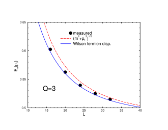
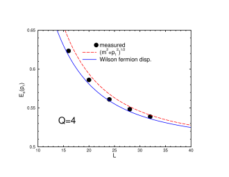
Figure 4: The electron energy at the non-zero lowest momentum ($p_{1}=2\pi/L$) as a function of the spatial size $L$ in lattice units. The left (right) panel for the $Q=3$ ($Q=4$) case. Full circles represent the measured values. The solid (dashed) curves are theoretical curves evaluated from the lattice (continuum-type) dispersion relation with the measured rest mass.

III.4 Diagonalization method

We are especially interested in the ${}^{1}S_{0}$ and ${}^{3}S_{1}$ states of the $e^{-}e^{+}$ system, where the electron-positron bound state (positronium) could be formed even in the Higgs phase. ${}^{1}S_{0}$ and ${}^{3}S_{1}$ positronium are described by the bilinear pseudo-scalar operator $\overline{\Psi}_{x}\gamma_{5}\Psi_{x}$ and vector operator $\overline{\Psi}_{x}\gamma_{\mu}\Psi_{x}$ respectively. Therefore, we may construct the four-point functions of electron-positron states based on the above operators. We are interested in not only the lowest level of two-particle spectra, but also the 2nd and 3rd lowest levels. In order to extract a few low-lying energy levels of two-particle system, we utilize the diagonalization method proposed by Lüscher and Wolff Luscher:1990ck . We consider three types of operators for this purpose:

$$\Omega_{P}(t) = \frac{1}{L^{3}}\sum_{\bf x}{\overline{\Psi}}({\bf x},t)\Gamma\Psi({\bf x},t),$$ (19)

$$\Omega_{W}(t) = \frac{1}{L^{6}}\sum_{{\bf x},{\bf y}}{\overline{\Psi}}({\bf y},t)\Gamma\Psi({\bf x},t),$$ (20)

$$\Omega_{M}(t) = \frac{1}{L^{6}}\sum_{{\bf x},{\bf y}}{\overline{\Psi}}({\bf y},t)\Gamma\Psi({\bf x},t)e^{i{\bf p}_{1}\cdot({\bf x}-{\bf y})},$$ (21)

where ${\bf p}_{1}=\frac{2\pi}{L}(1,0,0)$ and $\Gamma=\gamma_{5}$ ($\gamma_{\mu}$) for the ${}^{1}S_{0}$ (${}^{3}S_{1}$) $e^{-}e^{+}$ state. The first operator corresponds to a simple local-type operator where only the total momentum of two particles is fixed to be zero, but both the electron and the positron can carry non-zero relative momentum under the total momentum conservation. The second operator projects both the electron and the positron onto zero momentum, while the relative momentum of the $e^{-}e^{+}$ system is constrained to the non-zero lowest momentum ($p_{1}=|{\bf p}_{1}|=\frac{2\pi}{L}$) in the third operator. Therefore, we can expect that each type of operators has better overlap to a specific two-particle state: $n=0$ and $n=1$ scattering states have strong overlap with $\Omega_{W}$ and $\Omega_{M}$ respectively, while the bound state has the better overlap with $\Omega_{P}$ than $\Omega_{W}$ and $\Omega_{M}$.

We construct the $3\times 3$ matrix correlator from above three operators

$$G_{ij}(t)=\langle 0|\Omega_{i}(t)\Omega^{\dagger}_{j}(0)|0\rangle$$ (22)

and then employ a diagonalization of a transfer matrix $M(t,t_{0})$, which is defined by

$$M(t,t_{0})=G(t_{0})^{-1/2}G(t)G(t_{0})^{-1/2},$$ (23)

where $t_{0}$ is a reference time-slice. If only three states are propagating in the region $t>t_{0}$, the energies of three two-particle states $E_{\alpha}$ ($E_{2}>E_{1}>E_{0}$) are given by the eigenvalues of $M(t,t_{0})$:

$$\lambda_{\alpha}(t,t_{0})=e^{-(t-t_{0})E_{\alpha}}\;\;\;(\alpha=0,1,2),$$ (24)

where $E_{\alpha}$ is independent of $t_{0}$. An assumption that three low-lying states become effectively dominant for an appropriately large time-slice $t_{0}$, can be determined by checking the sensitivity of $E_{\alpha}$ with respect to variation of the reference time-slice $t_{0}$.

In this study, the random noise method is employed to calculate $\Omega_{p}$ source operators in Eq. (22) with the number of noises taken to be one. Technical details of this method are described in Ref. Aoki:2002ny ; Yamazaki:2004qb . We note that all contributions from disconnected diagrams in Eq. (22) are simply ignored in our numerical calculations.

IV Numerical results in the ${}^{1}S_{0}$ channel

In this section, we focus on numerical results in the ${}^{1}S_{0}$ channel of the $e^{-}e^{+}$ system. Results obtained in the ${}^{3}S_{1}$ channel will be separately discussed in the next section.

IV.1 Ground state of ${}^{1}S_{0}$

Let us begin with the ground state in the ${}^{1}S_{0}$ channel. It is not necessary to employ the diagonalization method for the spectroscopy of the ground state. We first show the effective mass plot for two diagonal components of the $3\times 3$ matrix correlator. Figs. 5 show the effective mass of the $PP$ correlator and the $WW$ correlator in simulations at spatial extent $L=28$ for $Q=3$ (left panel) and $Q=4$ (right panel). At a glance, there are apparent operator dependencies. A very clear plateau appears for the $WW$ correlator in the $Q=3$ case, while the same quality shows up for the $PP$ correlator in the $Q=4$ case. This drastic change in operator dependence strongly suggests a signature of bound-state formation in the $Q=4$ case, since the $WW$ correlator is expected to have a large overlap with the lowest ($n=0$) scattering state rather than the bound state. In addition, the energy of the ${}^{1}S_{0}$ ground state is close to the threshold energy ($2M_{e}\simeq 0.958$) in the case of $Q=3$, while there is a large energy gap between the ground state energy and the threshold energy ($2M_{e}\simeq 1.008$) in the case of $Q=4$. Therefore, we may naively conclude that the ground state in $Q=4$ is the ${}^{1}S_{0}$ positronium state .

To make a firm conclusion on this point, we next show the volume dependence of the ground state energy in Fig. 6. In the left panel ($Q=3$), we plot ground state energies measured at each $L$ together with the threshold energy as horizontal lines, which are estimated by $2M_{e}$ and its one standard deviation. An upward tendency of the $L$ dependence toward the threshold energy is clearly observed as spatial size $L$ increases. We also include a lower bound for the asymptotic solution of the scattering state. All data points are located well above this lower bound. From those observations, we can conclude that the observed ground state in the $Q=3$ is definitely the lowest ($n=0$) scattering state.

On the other hand, in the right panel ($Q=4$), all data points are located far below the threshold energy and also the lower bound for the asymptotic solution of the scattering state. Indeed, data are well fitted by the form:

$$E(L)=A+\frac{B}{L}\exp(-\gamma L),$$ (25)

which is inspired by the asymptotic solution of the bound state, Eq. (9). Finding $A\neq 2M_{e}$ directly indicates that the energy gap from the threshold remains finite in the infinite volume limit. We perform two types of fitting procedure with this form. First, a full three-parameter fit is employed. Second, we take into account a relation between two parameters $A$ and $\gamma$ according to Eq. (9). The parameter $A$ is the value of ground-state energy in the infinite volume, while $\gamma$ corresponds to the binding momentum related to the pole location of the $S$-matrix as $p^{2}=-\gamma^{2}(<0)$. Therefore, an explicit constraint between two parameters $A$ and $\gamma$ can be imposed through the relation $\gamma=\sqrt{M_{e}^{2}-A^{2}/4}$ referred to the measured electron mass $M_{e}$. Then a two-parameters fit is carried out. All fitting results are tabulated in Table. 4. Either procedure provides reasonable fits with about $\chi^{2}/{\rm d.o.f.}\sim 1$. The resulting values of $A$ in both fits are approximately consistent with each other, while some differences show up in other parameters.

We here stress that the obtained value of $A$ is significantly far from the threshold value $2M_{e}\simeq 1.008$ and therefore the energy gap $\Delta E=A-2M_{e}$ clearly remains finite in the infinite volume limit. A bound state of an electron and positron is certainly formed in simulations with charge-four electrons.

Figure 5: The effective masses in the ${}^{1}S_{0}$ channel on the lattice with $L=28$ as a function of the time-slice $t$ in lattice units. The left (right) panel is for $Q=3$ ($Q=4$) electron fields. Full circles (full squares) symbols are obtained from the $PP$ ($WW$) correlator.

Figure 6: Energies of ground states in the ${}^{1}S_{0}$ channel of the $e^{-}e^{+}$ system as a function of spatial lattice size $L$. In the left panel ($Q=3$), full circles are measured energies at each lattice size. Horizontal lines represent the threshold energy $2M_{e}$ and its 1 standard deviation (dashed lines). The dashed curve shows the lower boundary for the convergence of the large $L$ expansion formula around $q^{2}=0$ as Eq. (4). In the right ($Q=4$) panel, full circles are measured energies at each lattice size, and the solid (dashed) curve is the fitting result by using a form $E=A+B\exp(-\gamma L)/L$, which is inspired by the large $L$ expansion formula at infinite negative $q^{2}$ as Eq. (9), with (without) a constraint between two parameters ($A$ and $\gamma$).

Table 4: Fitting results for the ${}^{1}S_{0}$ ground state of $Q=4$ electron fields using a fitting form of Eq. (25). In the table, “Fit 1” and “Fit 2” stand for the fully three-parameters fit and the two-parameters fit with a constraint between $A$ and $\gamma$.

	$A$	$B$	$\gamma$	$\chi^{2}/{\rm d.o.f.}$
Fit 1	0.76395(26)	-0.78(30)	0.068(28)	0.87
Fit 2	0.76350(11)	-3.92(89)	constrained as $\sqrt{M_{e}^{2}-A^{2}/4}$	1.58

IV.2 Excited state of ${}^{1}S_{0}$

In the previous subsection, we confirm that the simulations with three-charge electrons provide the purely elastic scattering system without bound states (unbound system), while four-charge electrons give rise to at least one bound state as the ground state in the ${}^{1}S_{0}$ channel of the $e^{-}e^{+}$ system (bound system). We now can explore the difference of spectra between the unbound system ($Q=3$) and the bound system ($Q=4$).

We calculate the eigenvalues $\lambda_{\alpha}(t,t_{0})$ of the transfer matrix $M(t,t_{0})$ for $t_{0}=7$ at all $L$ except for $L=32$ where $t_{0}=9$ is chosen. First we show the effective mass plots for all three eigenvalues $\lambda_{\alpha}(t,t_{0}=7)$ in simulations at $L=28$ in Fig. 7. The diagonalization method with our chosen three operators successfully separates the first excited state and the second excited state from the ground state.

In the left panel ($Q=3$), the lowest and the second lowest states show very clear plateaus started from $t\simeq 5$, which is earlier than our reference time-slice $t_{0}$. The ground state and the first excited state correspond to the lowest ($n=0$) scattering state and the second lowest ($n=1$) scattering state. Those two-particle energies $E_{ee}^{0}$ and $E_{ee}^{1}$ are close to twice the single electron energies, $2E_{e}(p_{0})=2M_{e}$ and $2E_{e}(p_{1})$, respectively. Needless to say, the energy of the lowest state in the diagonalization method is consistent with the energy obtained by the $WW$ correlator. By detail analysis of the spectral amplitude (see, Table 5 and Appendix B), we confirm that the $WW$ correlator and the $MM$ correlator are dominant in $\lambda_{0}$ and $\lambda_{1}$ respectively as expected. Although the effective mass of the third eigenvalue $\lambda_{2}$ gradually approaches some plateau around $t\approx 20$, statistical errors becomes large in the plateau region. $\lambda_{2}$ is dominated by the $PP$ correlator, which can overlap with any relative momentum scattering state, so that the contamination from higher relative momentum ($n\geq 3$) scattering states is inevitable in the earlier time-slice.

For the bound system ($Q=4$), all three eigenvalues show clear plateaus started from $t\approx t_{0}=7$ in the effective mass plot. Again, the energy of the lowest state in the diagonalization method agrees well with the one obtained from the $PP$ correlator. The obtained eigenvectors also indicate that the $PP$ correlator is dominant in the $\lambda_{0}$ eigenvalue, while the second and third eigenvalues are mostly composed of the $WW$ correlator and the $MM$ correlator, respectively. As we mentioned, the $PP$ correlator possibly has overlap with any relative momentum scattering states. However, here, the $PP$ correlator has dominant overlap with the bound state as shown in Table 5. This is because the spectral weight of two-particle states relative to the single particle state, such as a bound state, could be suppressed in the $PP$ correlator by an inverse factor of the volume, $1/L^{3}$ .

Finally, a summary table of low-lying spectra in the ${}^{1}S_{0}$ channel in simulations at $L=28$ is given in Table 6.

Table 5: Summary of the normalized spectral weights $(A_{\alpha})_{i}$ in the ${}^{1}S_{0}$ channel on the lattice with $L=28$. A definition of the normalized spectral weights is described in Appendix B.

		ground state	1st excited state	2nd excited state
charge $Q$	operator $i$	$\alpha=0$	$\alpha=1$	$\alpha=2$
3	$P$	0.02166(72)	0.1324(96)	0.846(10)
	$W$	0.99735(37)	0.00177(11)	0.00088(31)
	$M$	0.001155(48)	0.9907(11)	0.0081(11)
4	$P$	0.9597(83)	0.0064(21)	0.0339(81)
	$W$	0.01567(69)	0.9841(14)	0.00018(78)
	$M$	0.0521(15)	0.0023(17)	0.9456(24)

Table 6: Summary of low-lying spectra in the ${}^{1}S_{0}$ channel on the lattice with $L=28$.

charge $Q$	eigenstate $\alpha$	energy $E_{\alpha}$	kinds of state
3	ground state ($\alpha=0$)	$E_{ee}^{0}$=0.95672(31)	$n=0$ scattering state
	1st excited state ($\alpha=1$)	$E_{ee}^{1}$=1.04062(41)	$n=1$ scattering state
4	ground state ($\alpha=0$)	$M_{\rm bs}$= 0.76370(17)	bound state
	1st excited state ($\alpha=1$)	$E_{ee}^{0}$= 1.0119(26)	$n=0$ scattering state
	2nd excited state ($\alpha=2$)	$E_{ee}^{1}$= 1.1044(53)	$n=1$ scattering state

Figure 7: The effective mass plots for each eigenvalue $\lambda_{\alpha}(t,t_{0})$ of the transfer matrix defined in Eq. (23) at a reference time-slice $t_{0}=7$ on the lattice with $L=28$. Full circles, squares and diamonds represent the ground state ($\alpha=0$), the first excited state ($\alpha=1$) and the second excited state ($\alpha=2$). The left (right) panel is for $Q=3$ ($Q=4$).

IV.3 Distinctive signatures of bound-state formation

IV.3.1 Sign of energy shift

Suppose that Lüscher’s finite size method reflects all of the essential nature of the scattering theory in the quantum mechanics; formation of the $S$-wave bound state is accompanied by an abrupt sign change of the scattering length. Thus, we can expect that the second lowest energy state, which corresponds to the lowest ($n=0$) scattering state, should be located near and above the threshold energy ($2M_{e}$) if a bound state is formed. This is quite in contrast with the case if there is no bound state: the second lowest energy state, which should be the $n=1$ scattering state, is located near below (above) the energy level of non-interacting two-particle system with non-zero lowest momentum as $2E_{e}(p_{1})$ in the attractive (repulsive) channel.

Here we show our observed $L$-dependence of the energy level of the second lowest state in Fig. 8. The data plotted appear in Table 7. In the left panel ($Q=3$), measured energy levels are very close to the $n=1$ threshold energy, which is given by twice the single electron energy at non-zero lowest momentum $p_{1}$. As the spatial size $L$ increases, the energy levels approach this $n=1$ threshold energy from below. This is consistent with a behavior of the $n=1$ scattering state predicted by Eq. (5) for the weakly attractive interaction without bound states. Therefore, one can identify the second lowest energy state as the $n=1$ scattering state for $Q=3$.

In the right panel ($Q=4$), an expected feature comes out. The horizontal line represents the $n=0$ threshold energy estimated by twice the electron rest mass. Clearly, the energy levels of the second lowest state approach this $n=0$ threshold energy from above. The energy shift from the threshold vanishes as the spatial size $L$ increases. Therefore, the second lowest energy state must be the $n=0$ scattering state. It is worth emphasizing that the sign of $\Delta E=E^{0}_{ee}-2M_{e}$ is opposite in the case of $Q=3$ where there is no bound state. Of course, this sign is directly related to the sign of the $S$-wave scattering length. Thus, our numerical simulations show that formation of the $S$-wave bound state is really accompanied by an abrupt sign change of the scattering length.

Furthermore, in Fig. 9, the volume dependence of the energy level of the third lowest state in the $Q=4$ case shows the “repulsive” feature as the $n=1$ scattering state even in the attractive channel. This is attributed to the consequence of Levinson’s theorem, which allows the case, $\tan\delta_{0}<0$, for the attractive interaction.

What is surprising here is that one of the most important features, namely Levinson’s theorem, in the quantum scattering theory is inherited in Lüscher’s finite size formula. Meanwhile, we realize what is a proper signature of bound state formation in finite volume on the lattice. Even in a single simulation at fixed $L$, we can distinguish the near-threshold bound state from the lowest ($n=0$) scattering state through determination of whether the second lowest state appears just above the threshold or near the $n=1$ energy level of non-interacting two-particle states.

Table 7: Energies of the ground state, the first excited state and the second excited state (only for $Q=4$), which are obtained by a single cosh fit with $2T$ periodicity, in the ${}^{1}S_{0}$ channel of the $e^{-}e^{+}$ system at five different lattice volumes $L^{3}\times 32$.

Spatial size	$Q=3$		$Q=4$
$L$	$E_{ee}^{0}$	$E_{ee}^{1}$	$M_{\rm bs}$	$E_{ee}^{0}$	$E_{ee}^{1}$
16	0.95183(40)	1.16903(55)	0.76231(26)	1.0242(52)	1.287(33)
20	0.95445(36)	1.10435(36)	0.76300(22)	1.0145(40)	1.197(14)
24	0.95644(37)	1.06590(36)	0.76314(22)	1.0126(34)	1.1318(93)
28	0.95672(31)	1.04062(41)	0.76370(17)	1.0119(26)	1.1044(53)
32	0.95767(32)	1.02440(49)	0.76359(20)	1.0113(32)	1.0888(68)

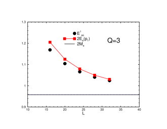
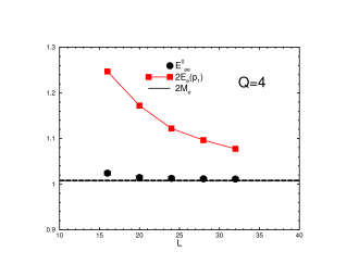
Figure 8: Energies of the first excited state in the ${}^{1}S_{0}$ channel of the $e^{-}e^{+}$ system as a function of spatial lattice size $L$. The left (right) panel is for $Q=3$ ($Q=4$). The horizontal line represents the threshold energy determined by $2M_{e}$. Full circles are measured energies for the first excited state. Solid curves with full squares shows twice of the single electron energy with non-zero smallest momentum $p_{1}=2\pi/L$.

Figure 9: Energies of the second excited state in the ${}^{1}S_{0}$ channel of the $e^{-}e^{+}$ system as a function of spatial lattice size $L$ for $Q=4$. All symbols are defined as in Fig. 8.

IV.3.2 Bound-state pole condition

As we discussed in Sec. II.2, the formation condition of the $S$-wave bound state, $\cot\delta_{0}(p)=i$, is definitely implemented in Lüscher’s phase-shift formula (3) at negative infinite $q^{2}$, which corresponds to the limit of $L\rightarrow\infty$. According to the original paper Luscher:1990ux , for negative $q^{2}$, we introduce the phase $\sigma_{0}(\kappa)$, which is defined by an analytic continuation of $\delta_{0}$ into the complex $p$ plane through the relation

$$\tan\sigma_{0}(\kappa)=-i\tan\delta_{0}(p),$$ (26)

where $\kappa=-ip$. Therefore, the bound-state pole condition in the infinite volume reads $\cot\sigma_{0}(\gamma)=-1$ for the binding momentum $\gamma$ Luscher:1990ux . As we pointed out in Sec. II.2, the finite volume correction on this condition is exponentially suppressed by the spatial extent $L$ in a finite box $L^{3}$:

$$\lim_{\kappa\rightarrow\gamma}\cot\sigma_{0}(\kappa) = -1+\sum_{\nu=1}^{\infty}\frac{N_{\nu}}{\sqrt{\nu}L\gamma}e^{-\sqrt{\nu}L\gamma}$$ (27)

$$= -1+\frac{6}{L\gamma}\left[e^{-L\gamma}+{\cal O}(e^{-\sqrt{2}L\gamma})\right],$$ (28)

where the factor $N_{\nu}$ is the number of integer vectors ${\bf n}\in Z^{3}$ with $\nu={\bf n}^{2}$. Therefore, if the bound state is formed, we may observe the phase $\sigma_{0}$ satisfies $\lim_{\kappa\rightarrow\gamma}\sigma_{0}(\kappa)=-\frac{\pi}{4}-\varepsilon_{L}$ where $\varepsilon_{L}(>0)$ vanishes as the spatial size $L$ increases.

We want to examine this bound-state pole condition numerically in the known bound system. As described previously, it is found that our simulation in the $Q=4$ case yields an $S$-wave bound state as the ground state in the ${}^{1}S_{0}$ channel. Thus, we determine the phase $\sigma_{0}$ from an energy level of the ground state in the $Q=4$ simulation by using Lüscher’s formula (3). We first calculate the relative momentum of two particles (electron-positron) from the measured energy level of the ground state $E_{ee}$ by matching with twice the single electron energy $2E_{e}(p)$. As we discussed in Sec.III.3.2, we prefer to use the lattice dispersion relation (18) for a formula of the single electron energy $E_{e}(p)$ in order to avoid lattice discretization errors as much as possible.

In Fig. 10, we plot the phase $\sigma_{0}$ in the ${}^{1}S_{0}$ channel as a function of $p^{2}(<0)$. The data plotted appear in Table 8. One can easily observe that the phase $\sigma_{0}$ approaches $-45$ deg. ($-\pi/4$) from below as the spatial size $L$ increases. Even at the smallest spatial extent $L=16$, the phase $\sigma_{0}$ is very close to $-\pi/4$. Needless to say, observed values of $p^{2}(=-\gamma^{2})$, which are related to the binding energy of the bound state, are almost insensitive to the spatial size $L$ within statistical errors. Thus, we confirm that our observed “bound state” in finite volume approximately fulfills the pole condition of the $S$-matrix.

A more rigorous way to test for bound-state formation would be to use an asymptotic formula for the finite volume correction to the pole condition as Eq. (28). In Fig. 11, we plot the value of $\cot\sigma_{0}$ versus the spatial lattice extent $L$ and show two fit results using Eq. (28) with different numbers of exponential terms (one term and three terms). As shown in Table 9, the optimum number of exponential terms, which yields a convergent result of $\gamma$, is about three. However, results with one term and three terms are quite consistent with each other because of rapid convergence. Then both fit curves in Fig. 11 reproduce all data points very well.

Table 8: Summary of the relative momentum squared $p^{2}$, the phase $\sigma_{0}$ and $\cot\sigma_{0}$ measured in the ${}^{1}S_{0}$ channel for $Q=4$ at five different lattice volumes $L^{3}\times 32$.

	16	20	24	28	32
$p^{2}$	$-$0.1252(17)	$-$0.1281(15)	$-$0.1245(15)	$-$0.1259(17)	$-$0.1252(18)
$\sigma_{0}$(deg.)	$-$45.1218(58)	$-$45.02012(99)	$-$45.00444(26)	$-$45.000860(65)	$-$45.000186(17)
$\cot\sigma_{0}$	$-$0.99576(20)	$-$0.999298(35)	$-$0.9998449(91)	$-$0.9999700(23)	$-$0.99999352(58)

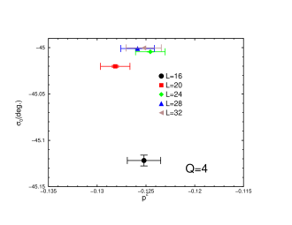
Figure 10: Phase $\sigma_{0}$ as a function of relative momentum squared $p^{2}$ in the $Q=4$ simulation. Different symbols represent the values obtained from simulations with different spatial lattice sizes.

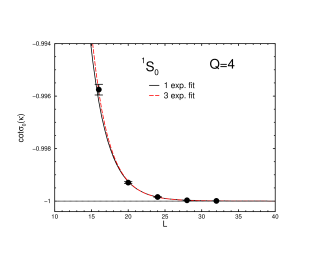
Figure 11: $\cot\sigma_{0}$ in the ${}^{1}S_{0}$ channel for $Q=4$ as a function of the spatial lattice size $L$. The solid (dashed) curve represents a fitting result using Eq. (28) with only a leading exponential term (three exponential terms).

Table 9: Fitting results for the bound-state pole condition in the ${}^{1}S_{0}$ channel for $Q=4$ using Eq. (28) with variation of the number of exponential terms.

fitting range ($L$)	# of exp. terms	$\gamma$	$\chi^{2}/{\rm d.o.f.}$
16-32	1	0.3524(11)	1.79
	2	0.3547(11)	0.86
	3	0.3549(11)	0.85
	4	0.3549(11)	0.85

IV.4 $e^{-}e^{+}$ elastic scattering phase shifts

Finally, we evaluate the elastic scattering phase shift of both the unbound system ($Q=3$) and the bound system ($Q=4$) using Lüscher’s formula (3).

IV.4.1 Unbound system ($Q=3$)

In the $Q=3$ case, as we described previously, there is no bound state. The ground state and the first excited state correspond to $n=0$ and $n=1$ scattering states respectively and those energy levels are successfully separated by the diagonalization method. Then we can measure the scattering phase shifts $\delta_{0}(p)$ at two different kinematical points, which correspond to the relative momenta of the two particles (electron-positron) $p$ for both $n=0$ and $n=1$ scattering states. However, as for the $n=0$ scattering state, the relative momentum squared is negative ($p^{2}<0$) because of the attractive interaction between the electron and the positron. Therefore, we only access the phase $\sigma_{0}$ from the energy level of the $n=0$ scattering state in this sense. However, we consider the effective-range expansion for the scattering phase as $p\cot\delta_{0}(p)=\frac{1}{a_{0}}+\frac{1}{2}r_{0}p^{2}+{\cal O}(p^{4})$ in the vicinity of zero relative momentum. We then assume this expansion is still valid for negative $p^{2}$. Therefore, we may translate the phase $\sigma_{0}$ to the scattering phase shift $\delta_{0}$ in the following relation

$$\lim_{\kappa\rightarrow 0}\kappa\cot\sigma_{0}(\kappa)=\lim_{p\rightarrow 0}p\cot\delta_{0}(p)=\frac{1}{a_{0}}\;.$$ (29)

In other words, we approximately identify the value of $\sigma_{0}(\kappa)$ at $p^{2}=-\kappa^{2}$ to the scattering phase shift $\delta_{0}(p)$ at $p^{2}=+\kappa^{2}$. On the other hand, the relative momentum squared of the $n=1$ scattering state is definitely positive so that we directly access the scattering phase shift $\delta_{0}$ through Lüscher’s formula without any approximation .

We plot scattering phase shifts measured from both $n=0$ and $n=1$ scattering-state energies in the $Q=3$ case as a function of the relative momentum squared in the left panel of Figs. 12 and in the left panel of Figs. 13 following the above descriptions.

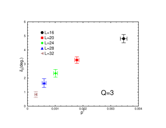
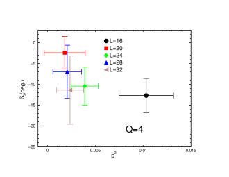
Figure 12: Scattering phase shifts $\delta_{0}$ from the energy level of the $n=0$ scattering states (corresponding to the ground state for $Q=3$ and the first excited state for $Q=4$). The horizontal axis is the squared relative momentum of the $e^{-}e^{+}$ system. The left (right) panel is for $Q=3$ ($Q=4$). Different symbols represent the values obtained from simulations with different spatial lattice sizes. Remark that the sign of $\delta_{0}$ for $Q=4$ is opposite to that for $Q=3$.

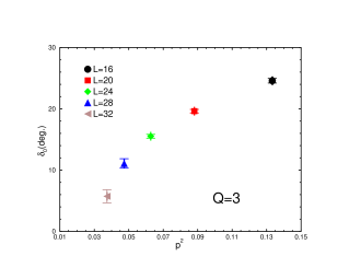
Figure 13: Scattering phase shifts $\delta_{0}$ from the energy level of the $n=1$ scattering states (corresponding to the first excited state for $Q=3$ and the second excited state for $Q=4$). The horizontal axis is the squared relative momentum of the $e^{-}e^{+}$ system. The left (right) panel is for $Q=3$ ($Q=4$). Different symbols represent the values obtained from simulations with different spatial lattice sizes. Remark that the sign of $\delta_{0}$ for $Q=4$ is opposite to that for $Q=3$.

IV.4.2 Bound system ($Q=4$)

In the $Q=4$ case, it is found that the ground state corresponds to the $S$-wave bound state. As we discussed in Sec. III.2, the first and the second excited states should be $n=0$ and $n=1$ scattering states, respectively. Although we can not access any information of the scattering phase shift from the energy level of the ground state, we instead determine the scattering phase shift from the energy levels of the first and second excited states. In contrast to the purely scattering system without bound states ($Q=3$), the relative momentum squared is given as the positive value even from the lowest ($n=0$) scattering state, which appears above the threshold. Therefore, we can simply evaluate the phase shift $\delta_{0}$ using Lüscher’s formula with measured $p^{2}$.

In the right panels of both Figs. 12 and Figs. 13, we plot our measured scattering phase shifts for $Q=4$ versus the relative momentum squared. Here, the values of the phase shift $\delta_{0}$ are simply restricted to the interval $(-\frac{\pi}{2},\frac{\pi}{2}]$. Therefore, we observe negative phase shift $\delta_{0}$ despite an attractive interaction between the electron and the positron. Roughly speaking, the phase shift $\delta_{0}$ monotonically increases as $p^{2}$ decreases and approaches zero toward zero momentum squared. It implies that the $S$-wave scattering length $a_{0}$ is negative for the bound system ($Q=4$).

IV.4.3 Scattering amplitude

Here, we define an $S$-wave scattering amplitude $T(p)$

$$T(p)=\frac{\tan\delta_{0}(p)}{p}\frac{E_{ee}}{2},$$ (30)

where $E_{ee}$ represents the measured energy of the scattering state. Analyticity of the scattering amplitude $T(p)$ allows us to consider the following fit ansätz:

$$T(p)=d_{0}+d_{1}p^{2}+d_{2}p^{4}+d_{3}p^{6}+d_{4}p^{8},$$ (31)

which is a simple polynomial function in the relative momentum squared $p^{2}$. The results of the fit are summarized in Table. 10. For $Q=4$, a linear fit with respect to $p^{2}$ is enough to describe the data with reasonable $\chi^{2}/{\rm d.o.f.}$, while the fourth order polynomial fit still yields large $\chi^{2}/{\rm d.o.f.}$ in the case of $Q=3$. The latter point will be discussed before this session is closed.

We then obtain a global $p^{2}$-dependence of the phase shift $\delta_{0}$ in the measured region of $p^{2}$, which is deduced from fitted results of the scattering amplitude. We show all measured phase shifts $\delta_{0}$, which are obtained from the energy levels of both $n=0$ and $n=1$ scattering states, in Figs. 14. Solid curves represent inferred $p^{2}$-dependence of the phase shift with the band of their errors.

In the right panel ($Q=4$), we take into account the modulo-$\pi$ ambiguity in determination of the phase shift $\delta_{0}$ because of the bound system and raise the phase shift by an additional $\pi$ in order to fulfill Levinson’s theorem. That is why the phase shift data starts from $\pi$ and monotonically decreases as $p^{2}$ increases. All data are well covered with rather wide bands of error associated with the global fit.

On the other hand, in the left panel ($Q=3$), two data sets determined from energy levels of $n=0$ and $n=1$ scattering states seem not to be smoothly connected with each other due to the lower data points from the $n=1$ scattering state at $L=28$ and 32. We remark that although statistical errors on all points are rather small, a hidden and large systematic error stems from an order ${\cal O}(a)$ lattice artifact in the determination of $p^{2}$. As we discussed in Sec. III.3.2, we have used the lattice dispersion relation in the analysis of the scattering phase shift. The continuum-type dispersion relation yields smaller estimations of $p^{2}$ than those obtained from the lattice dispersion relation. These differences are far beyond statistical errors, especially for $p^{2}$ obtained from the $n=1$ energy level in the $Q=3$ case. Furthermore, discrepancies are largely enhanced in determination of the scattering phase shift through the Lüscher finite formula. The scattering phase shift from the $n=1$ energy level for $Q=3$ typically increases by about a factor of two, if the continuum-type dispersion relation is utilized in the whole analysis.

At the low-energy limit, the scattering amplitude becomes

$$\lim_{p\rightarrow 0}T(p)=a_{0}M_{e}.$$ (32)

Therefore, the fitting parameter $d_{0}$ in Eq. (31) is associated with the scattering length $a_{0}$. We then obtain the scattering lengths as $a_{0}=1.46(5)$ for $Q=3$ and $-2.28(40)$ for $Q=4$ in lattice units, which are much smaller than our utilized lattice sizes ($L\geq 12$). Needless to say, the sign of the scattering length for $Q=4$ is opposite to that for $Q=3$ due to formation of one bound state in the case of $Q=4$.

Table 10: Fitting results for the scattering amplitude for $Q=3$ and $Q=4$ using Eq. (31).

charge $Q$	$d_{0}$	$d_{1}$	$d_{2}$	$d_{3}$	$d_{4}$	$\chi^{2}/$d.o.f.
3	0.697(26)	$-$33.8(7.4)	102(25)$\times 10$	$-$103(28)$\times 10^{2}$	34(10)$\times 10^{3}$	7.26
4	$-$1.15(20)	$-$4.6(7.3)	—	—	—	0.52

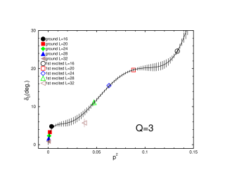
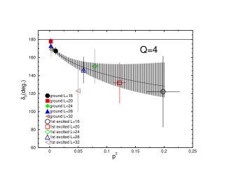
Figure 14: All measured scattering phase shift $\delta_{0}$ as a function of the squared relative momentum. As for the $Q=4$ case (the left panel) where the formation of bound state is observed, the scattering phase shifts $\delta_{0}$ are shifted as $\delta_{0}\rightarrow\delta_{0}+\pi$ according to Levinson’s theorem. Solid curves represent the fitting results with the band of their errors.

V Numerical results in the ${}^{3}S_{1}$ channel

V.1 Low-lying spectra in the $Q=4$ case

The ${}^{3}S_{1}$ spectroscopy has been done in exactly the same way as the ${}^{1}S_{0}$ case by using the bilinear vector operator $\overline{\Psi}_{x}\gamma_{\mu}\Psi_{x}$. As for the Lorentz indices, we take an average over the spatial indices so as to gain possible reduction of statistical errors. After we perform the diagonalization method with the $3\times 3$ matrix correlator constructed with three operators in Eq.(21), we get the energy spectra of both the ground state and the first excited state.

In the $Q=4$ case, we have concluded that one bound state is formed in the ${}^{1}S_{0}$ channel as described in the previous section. The binding energy $B=|M_{\rm bs}-2M_{e}|$ is rather large as $B\approx M_{e}/2$. The observed bound state should be a “tightly bound state” rather than a “loosely bound state”. On the other hand, the mass of the ${}^{3}S_{1}$ bound state is naturally expected to be higher than the ${}^{1}S_{0}$ bound state due to the hyperfine-splitting interaction. Indeed, we observe that the ground state in the ${}^{3}S_{1}$ channel is much closer to the threshold energy as $|\Delta E|\approx M_{e}/25$. Although the energy level of the ground state is too near the threshold to be simply identified as a bound state, we may expect that the ${}^{3}S_{1}$ ground state is a near-threshold bound state or a loosely bound state. Needless to say, to draw a solid conclusion, we need more rigorous signatures of bound-state formation in the ${}^{3}S_{1}$ channel.

We employ the diagonalization method to separate the first excited state from the ground state. Fig. 15 shows $L$-dependence of energies of the ground state and the first excited state in the ${}^{3}S_{1}$ channel for $Q=4$. The horizontal axis is the spatial size $L$ and the vertical axis is the energy of the ground state (full circles) or the first excited state (full diamonds). The horizontal lines represent the threshold energy of the $e^{-}e^{+}$ system together with the 1 standard deviation, which is evaluated as twice the measured electron mass. Although it seems that the ground state has no appreciable finite-size effect for $L$ larger than 20, the ${}^{3}S_{1}$ ground state lies too close to the threshold energy to be assured of bound-state formation.

As shown in Sec. IV.3, the distinctive signature of bound states is given by an information of the excited state spectra: if a bound state is formed, the lowest ($n=0$) scattering state could appear just above the threshold ($2M_{e}$), but far from the $n=1$ energy level of non-interacting two-electron system ($2E_{e}(p_{1})$). Indeed, we observe that the first excited state appears just above the threshold and its energy rapidly approaches the threshold as spatial size $L$ increases. The first excited state can be clearly distinguished from the $n=1$ scattering state. Of course, it indicates that the ground state should not be the lowest scattering state. Thus, we can conclude: the ${}^{3}S_{1}$ ground state should be the $S$-wave bound state, of which formation clearly induces the sign of the scattering length to change. Therefore, the lowest ($n=0$) scattering state approaches the threshold from above, the same as the repulsive system in the attractive channel. This result shows that our proposal could be quite promising for identifying a near-threshold bound state or a loosely bound state such as a hadronic molecular state in a finite box on the lattice.

Figure 15: Energies of the ground state and the first excited state in the ${}^{3}S_{1}$ channel of the $e^{-}e^{+}$ system as a function of spatial lattice size for $Q=4$. The horizontal line represents the threshold energy determined by $2M_{e}$. Full circles and full diamonds are measured energies for the ground state and the first excited state respectively. A solid curve with full squares shows twice of the single electron energy with non-zero smallest momentum $p_{1}=2\pi/L$.

V.2 Bound-state pole condition

Next, we evaluate the phase $\sigma_{0}$ from the energy level of the ground state through the phase-shift formula (3) as we did in Sec. IV.3.2. All results measured at five different lattice volumes $L^{3}\times 32$ are tabulated together with results of $p^{2}$ and $\cot\sigma_{0}$ in Table 11. Indeed, we observe that the phase $\sigma_{0}$ gradually approaches $-45$ deg. ($-\pi/4$) as spatial lattice extent $L$ increases. However, $\sigma_{0}$ is not really close to $-45$ deg. even at the largest volume ($L=32$), in comparison to $\sigma_{0}$ from the smallest volume ($L=16$) in the ${}^{1}S_{0}$ channel. In this sense, it is hard to judge how large of a lattice size is enough to deal with the asymptotic solution of the bound state even in finite volume. Thus, we should examine the $L$-dependence of the specific quantity, $\cot\sigma_{0}$, by reference to Eq. (28), where the finite volume corrections on the bound-state pole condition are theoretically predicted.

As shown in Fig. 16, the values of $\cot\sigma_{0}$ are plotted as a function of spatial lattice extent $L$. Full circles are measured value at five different lattice volumes. The solid and dashed curves represent fit results with a single leading exponential term and six exponential terms in Eq. (28). The four data points in the region $20\leq L\leq 32$ are used for those fits. The fitting with the six exponential terms yields a convergent result of $\gamma$ as shown in Table 12. Either fit curves in Fig. 16 reproduce all data points except for data at the smallest $L$. Indeed, the resulting $\chi^{2}/{\rm d.o.f.}$ is no longer reasonable as $\chi^{2}/{\rm d.o.f.}\approx 3$ if the data point at $L=16$ is used. Therefore, the ground state at least for $L\geq 20$ can be identified as a bound state without ambiguity.

Table 11: Summary of the relative momentum squared $p^{2}$, the phase $\sigma_{0}$ and $\cot\sigma_{0}$ measured in the ${}^{3}S_{1}$ channel for $Q=4$ at five different lattice volumes $L^{3}\times 32$.

	16	20	24	28	32
$p^{2}$	$-$0.0255(26)	$-$0.0158(23)	$-$0.0167(23)	$-$0.0148(26)	$-$0.0120(34)
$\sigma_{0}$(deg.)	$-$56.1(2.9)	$-$57.1(4.5)	$-$49.2(1.5)	$-$47.6(1.2)	$-$47.2(1.6)
$\cot\sigma_{0}$	$-$0.673(73)	$-$0.65(11)	$-$0.864(45)	$-$0.914(38)	$-$0.926(53)

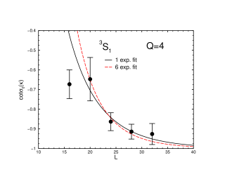
Figure 16: $\cot\sigma_{0}$ in the ${}^{3}S_{1}$ channel for $Q=4$ as a function of the spatial lattice size $L$. The solid (dashed) curve represents a fitting result using Eq. (28) with only a leading exponential term (six exponential terms).

Table 12: Fitting results for the bound-state pole condition in the ${}^{3}S_{1}$ channel for $Q=4$ using Eq. (28) with variation of the number of exponential terms.

fitting range ($L$)	# of exp. terms	$\gamma$	$\chi^{2}/{\rm d.o.f.}$
20-32	1	0.1109(60)	0.24
	2	0.1218(57)	0.24
	3	0.1236(56)	0.25
	4	0.1242(55)	0.25
	5	0.1251(55)	0.26
	6	0.1256(54)	0.27
	7	0.1256(54)	0.27

VI Summary and conclusion

In this paper, we have discussed signatures of bound-state formation in finite volume via Lüscher finite size method. Assuming that the phase-shift formula inherits all aspects of the quantum scattering theory, we can propose a novel approach to distinguish a “loosely bound state” from the lowest scattering state, which is located below the threshold in finite volume in the case of attractive two-particle interaction. According to the quantum scattering theory, the $S$-wave scattering length is positive ($a_{0}>0$) in the attractive channel, if the attraction is not strong enough to give rise to a bound state. However, the sign of the scattering length turns out to be opposite ($a_{0}<0$) once the bound state is formed. This fact provides us a distinctive identification of a loosely bound state even in finite volume through the observation of the lowest scattering state that is above the threshold. We also reconsider the bound-state pole condition in finite volume, based on the phase-shift formula in the Lüscher finite size method. We find that the bound-state pole condition is fulfilled only in the infinite volume limit, but its modification by finite size corrections is exponentially suppressed by the spatial lattice size $L$.

To check the above theoretical considerations, we have performed numerical simulations to calculate the positronium spectrum in compact scalar QED, where the short-range interaction between an electron and a positron is realized in the Higgs phase. We introduce the fictitious $Q$-charged electron to control the strength of this interparticle force and then can adjust the charge $Q$ to give rise to the $S$-wave bound states such as ${}^{1}S_{0}$ and ${}^{3}S_{1}$ positronium. We choose two parameter sets $(Q,\kappa)$ that lead to an unbound $e^{-}e^{+}$ system ($Q=3$) and a bound $e^{-}e^{+}$ system ($Q=4$) at approximately the same mass of a single electron. We observe the following signatures of the bound-state formation, some of which are related to our theoretical proposals, in our numerical simulations.

• The lowest scattering state has better overlap with the wall-wall correlator than the point-point correlator. This tendency is inverted in the case of the bound state.

• The sign of the $S$-wave scattering length turns out to be opposite (repulsive-like) even in the attractive channel, once the bound state is formed.

• In the bound system, the phase $\sigma_{0}$, which is related to the scattering phase $\delta_{0}(p)$ and analytically continued into the complex $p$-plane, is near $-45$ deg. ($-\pi/4$) which is associated with the pole condition of the $S$-matrix.

• The deviation from the pole condition, $\cot\sigma_{0}=-1$, in finite volume is well described by a finite series of exponentially convergent terms with respect to the spatial extent $L$ scaled by the binding momentum $\gamma$.

In particular, we regard the second point, the bound-state formation induces the sign of the scattering length to be changed, as crucially important for identifying a “loosely bound state”. This is because one can distinguish it from the lowest scattering state even in a single simulation at fixed $L$ through determination of whether the second lowest energy state appears just above the threshold or near the $n=1$ energy level of non-interacting two-particle system. We also emphasis that Lüscher’s phase-shift formula properly reflects one of the most essential features of the quantum scattering theory, namely Levinson’s theorem.

Appendix A: Sensitivity of mass spectra to spatial boundary conditions

Kinematics of two-particle states on the lattice should be sensitive to choice of the spatial boundary condition. In many literatures, this particular point is often discussed and sometimes applied to explore hadronic or non-leptonic decay processes DeGrand:1990ip ; Kim:2002np or to search exotic hadrons Sasaki:2003gi ; Csikor:2003ng on the lattice. The main point is that the total energy of two-particle states, which is roughly estimated by a sum of the energy of non-interacting two particles, depends on the spatial size $L$ unless the relative momentum of two particles is zero. Of course, this is because all momenta on the lattice are discretized in units of $2\pi/L$. Here, we have considered the $e^{-}e^{+}$ system. The total energy of electron-positron states is approximately estimated by using the naive relativistic dispersion relation in the following.

$$E_{ee}^{n}\sim 2E_{e}(p_{n})=2\sqrt{M_{e}^{2}+{\bf p}_{n}^{2}}.$$ (33)

The discrete momenta of a single electron are obtained as ${\bf p}_{n}=\frac{2\pi}{L}{\bf n}$ for the periodic boundary condition (P.B.C.) and ${\bf p}_{n}=\frac{\pi}{L}(2{\bf n}+1)$ for the anti-periodic boundary condition (A.P.B.C.). In the anti-periodic boundary condition, zero relative-momentum is not kinematically allowed, so that the lowest energy of two-particle scattering states is expected to be very sensitive to the spatial lattice size. In other words, different types of spatial boundary conditions (periodic or anti-periodic) exhibit different energy levels of the two-particle scattering states even at the fixed spatial size, while a mass of $e^{-}e^{+}$ bound states (positronium states) should be insensitive to the spatial boundary condition for the electron fields . For an example, in the $n=0$ case, we obtain

$$E_{ee}^{0}\sim 2E_{e}(p_{0})=\left\{\begin{array}[]{ll}2M_{e}&\mbox{(P.B.C. for all spatial directions)},\\ \\ 2\sqrt{M_{e}^{2}+3\cdot\left(\frac{\pi}{L}\right)^{2}}&\mbox{(A.P.B.C. for all spatial directions)},\end{array}\right.$$ (34)

which imply an inequality $E^{0}_{ee}({\rm P.B.C.})<E^{0}_{ee}({\rm A.P.B.C.})$. In general, we can expect that $E^{n}_{ee}({\rm P.B.C.})<E^{n}_{ee}({\rm A.P.B.C.})$ is always fulfilled.

Recently, such sensitivity of spatial boundary condition is often utilized to distinguish between two-particle scattering states and a single-particle state (a bound state or a resonance state) Ishii:2004qe ; Iida:2006mv . However, there is no rigorous test of whether this approach is adequate for such purpose so far. In this subsection, we examine this approach in our simulated $e^{-}e^{+}$ system.

We use the following operators under the anti-periodic spatial boundary condition for electron fields:

$$\Omega_{P}(t) = \frac{1}{L^{3}}\sum_{\bf x}{\overline{\Psi}}({\bf x},t)\gamma_{5}\Psi({\bf x},t),$$ (35)

$$\Omega_{M_{0}}(t) = \frac{1}{L^{6}}\sum_{{\bf x},{\bf y}}{\overline{\Psi}}({\bf y},t)\gamma_{5}\Psi({\bf x},t)e^{i{\bf p}_{0}\cdot({\bf x}-{\bf y})},$$ (36)

$$\Omega_{M_{1}}(t) = \frac{1}{L^{6}}\sum_{{\bf x},{\bf y}}{\overline{\Psi}}({\bf y},t)\gamma_{5}\Psi({\bf x},t)e^{i{\bf p}_{1}\cdot({\bf x}-{\bf y})},$$ (37)

where ${\bf p}_{0}=\frac{\pi}{L}(1,1,1)$ and ${\bf p}_{1}=\frac{\pi}{L}(3,1,1)$. The first operator is a simple local-type operator. The second and third operators project both the electron and the positron on non-zero lowest momentum ($|{\bf p}_{0}|=\frac{\sqrt{3}\pi}{L}$) and non-zero second lowest momentum ($|{\bf p}_{1}|=\frac{\sqrt{11}\pi}{L}$), respectively. We can expect that $n=0$ and $n=1$ scattering states have strong overlap with $\Omega_{M_{0}}$ and $\Omega_{M_{1}}$, while the bound state has the better overlap with $\Omega_{P}$ than $\Omega_{M_{0}}$ and $\Omega_{M_{1}}$.

Figs. 17 show the effective mass plots of the $PP$, $M_{0}M_{0}$ and $M_{1}M_{1}$ correlators in simulations at $L=28$ for $Q=3$ (the left panel) and $Q=4$ (the right panel) in the ${}^{1}S_{0}$ channel. There is a similarity between Figs. 5 (P.B.C.) and Figs. 17 (A.P.B.C.). Very clear plateaus are given by the $M_{0}M_{0}$ correlator in the $Q=3$ case and the $PP$ correlator in the $Q=4$ case in Figs. 17, while the same quality shows up for the $WW$ correlator in the $Q=3$ case and the $PP$ correlator in the $Q=4$ case in Figs. 5. In either P.B.C. and A.P.B.C. cases, the $PP$ correlator strongly overlap with the $Q=4$ ground state, which has already been identified as the bound state in Sec. IV. Both $WW$ and $M_{0}M_{0}$ correlators are expected to have large overlap with the lowest ($n=0$) scattering state under each spatial boundary condition. A main difference between Figs. 5 (P.B.C.) and Figs. 17 (A.P.B.C.) is that the $PP$ ($M_{1}M_{1}$) correlator for $Q=3$ ($Q=4$) in the A.P.B.C. approaches the plateau much faster than the P.B.C. cases. This is simply because $E^{n}_{e}({\rm A.P.B.C.})$ is larger than $E^{n}_{e}({\rm P.B.C.})$ and then propagations of non-ground state can die out more quickly in the A.P.B.C. case than the P.B.C. case. Indeed, the $M_{1}M_{1}$ correlator approaches the plateau faster than the $M_{0}M_{0}$ correlator in the left panel ($Q=4$) of Fig. 17 since the $M_{1}M_{1}$ correlator hardly overlaps with the $n=0$ scattering state as shown in the right panel ($Q=3$) of Fig. 17.

We finally employ the diagonalization method to extract the ground states in both $Q=3$ and $Q=4$ through the same procedure described in Sec. IV.2. Then we compare ground state energies for both $Q=3$ and $Q=4$ in the P.B.C. with those in the A.P.B.C. in Figs. 18. The left panel ($Q=3$), the effective mass of the ground state is clearly shifted up in changing from P.B.C. to A.P.B.C., while the plateau of the ground state doesn’t change between P.B.C. and A.P.B.C. cases in the right panel ($Q=4$). An energy shift in the $Q=3$ case is consistent with an estimation of $2(E^{0}_{e}({\rm A.P.B.C.})-E^{0}_{e}({\rm P.B.C.}))$. We certainly confirm that the scattering state ($Q=3$) is sensitive to the spatial boundary condition, while the bound state has no dependence of the spatial boundary condition for the electron fields.

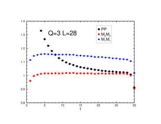
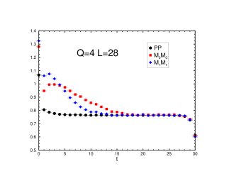
Figure 17: The effective masses in the ${}^{1}S_{0}$ channel on the lattice with $L=28$ as a function of the time-slice $t$ in lattice units The anti-periodic boundary condition is imposed in the spatial direction. The left (right) panel is for $Q=3$ ($Q=4$) electron fields. Full circles, full squares and full diamonds are obtained from $PP$, $M_{0}M_{0}$ and $M_{1}M_{1}$ correlators respectively.

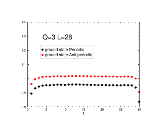
Figure 18: The effective mass plots for the largest eigenvalue $\lambda_{\alpha}(t,t_{0}=7)$, which corresponds to the lowest energy state, on the lattice with $L=28$ in the ${}^{1}S_{0}$ channel. The left (right) panel is for $Q=3$ ($Q=4$). Full circles (full squares) represent the ground states from simulations with periodic (anti-periodic) boundary conditions for electron fields in the spatial direction.

Appendix B: Volume dependence of the spectral weight

The spectral decomposition of the matrix correlator is given by

$$G_{ij}(t)=\sum_{\alpha=0}(v_{\alpha})_{i}(v^{*}_{\alpha})_{j}e^{-E_{\alpha}t}$$ (38)

with the spectral amplitude $(v_{\alpha})_{i}={\langle 0|\Omega_{i}|\alpha\rangle}_{V}$. A subscript in a ket ${|\alpha\rangle}_{V}$ stands for finite volume $V=L^{3}$. Remark that the finite-volume states ${|\alpha\rangle}_{V}$ are normalized to unity. The spectral amplitudes are given by solving the following equations Gockeler:1994rx

$$\sum_{i}(w_{\alpha})_{i}(v^{*}_{\beta})_{i}=\delta_{\alpha\beta}e^{E_{\alpha}t_{0}/2},$$ (39)

where $(w_{\alpha})_{i}$ is an $i$ component of vectors ${\bf w}_{\alpha}$, which are determined through the following generalized eigenvalue problem Gockeler:1994rx :

$$G(t){\bf w}_{\alpha}=\lambda_{\alpha}(t,t_{0})G(t_{0}){\bf w}_{\alpha}.$$ (40)

To solve this eigenvalue equation, we have employed a diagonalization of the transfer matrix $M(t,t_{0})=G^{-1/2}(t_{0})G(t)G^{-1/2}(t_{0})$, which provides the same eigenvalues $\lambda_{\alpha}(t,t_{0})=e^{-E_{\alpha}(t-t_{0})}$ of Eq.(40)

$$M(t,t_{0}){\bf u}_{\alpha}=\lambda_{\alpha}(t,t_{0}){\bf u}_{\alpha}$$ (41)

with the orthonormal eigenvectors ${\bf u}_{\alpha}=G^{1/2}(t_{0}){\bf w}_{\alpha}$, if $G(t)$ is an Hermite matrix Gockeler:1994rx . The relative overlap between the chosen operator $\Omega_{i}$ and energy eigenstates ($\alpha=0,1,2,\cdot\cdot\cdot$) can be determined by the squared normalized amplitudes (the normalized spectral weights)

$$(A_{\alpha})_{i}=\frac{|(v_{\alpha})_{i}|^{2}}{\sum_{\alpha}|(v_{\alpha})_{i}|^{2}}.$$ (42)

The normalized spectral weights calculated in simulations at $L=28$ are tabulated in Table 5 as typical examples.

Here, we remind that the finite-volume states are normalized to unity, regardless of whether the single particle state or the multi-particle state. Suppose the eigenstate $\alpha$ is a single particle state, we simply obtain the correspondence between the finite-volume and the infinite-volume states:

$${|\alpha\rangle}_{V}=\frac{1}{\sqrt{2E_{\alpha}V}}{|\alpha\rangle}_{\infty}\;\;\;(\mbox{single particle state}),$$ (43)

where ${|\alpha\rangle}_{\infty}$ is normalized as $2E_{\alpha}$ particles per unit volume. On the other hand, if the eigenstate $\alpha$ is a two-particle state, the correspondence factor between ${|\alpha\rangle}_{\infty}$ and ${|\alpha\rangle}_{V}$ should depend on dynamics between two particles. Such corrected factor is explicitly derived by Lellouch and Lüscher (denoted in the following by LL) to determine the physical $K\rightarrow\pi\pi$ amplitude from the finite volume calculation Lellouch:2000pv . Here, we consider the LL-factor only in the non-interacting case, where the scattering phase shift between two particles is taken to be zero, for a simplicity, and then obtain the following correspondence between ${|\alpha\rangle}_{\infty}$ and ${|\alpha\rangle}_{V}$ for $S$-wave two-particle states Lellouch:2000pv ; Lin:2001ek :

$${|\alpha\rangle}_{V}\propto\frac{1}{E_{\alpha}V}{|\alpha\rangle}_{\infty}\;\;\;(\mbox{two-particle state}),$$ (44)

which indicates that observed spectral amplitudes $(v_{\alpha})_{i}$ for the local-type operator ($i=P$) are proportional to $1/\sqrt{V}$ for the single particle state and proportional to $1/V$ for the $S$-wave two-particle state, since the physical spectral amplitude $\langle 0|\Omega_{P}{|\alpha\rangle}_{\infty}$ in the case of the local-type operator should not depend on the size of the spatial volume $V=L^{3}$.

Let us consider the volume dependence of the spectral amplitude of the ground state with the local-type operator $\Omega_{P}$. In Fig. 19, we plot the finite-volume spectral weight $|\langle 0|\Omega_{P}{|\alpha=0\rangle}_{V}|^{2}$ scaled by $V^{2}$ for $Q=3$ and by $V$ for $Q=4$ as a function of spatial lattice size $L$. Recall that $Q=3$ is the unbound system, while $Q=4$ is the bound system. No appreciable $L$-dependence is observed in either cases. This indicates that the finite-volume spectral weight for the local-type operator has a specific volume dependence according to whether the single particle state or the two-particle state. In other words, each contribution from two-particle states (scattering states) relative to the single particle state is suppressed by a inverse of the volume factor, $1/L^{3}$ in the $PP$ correlator.

Figure 19: The volume dependence of the spectral weight of the ${}^{1}S_{0}$ ground state with the local-type operator $\Omega_{P}$. We plot $|\langle 0|\Omega_{P}|\alpha=0\rangle|^{2}$ scaled by $V^{2}=L^{6}$ for $Q=3$ (full squares) and by $V=L^{3}$ for $Q=4$ (full circles) as a function of spatial lattice size $L$. Remind that $Q=3$ ($Q=4$) is the unbound system (the bound system), where the $n=0$ scattering state (the bound state) is the ground state. There is no appreciable $L$-dependence in either cases.

References

- (1) See, e.g., E. Klempt, arXiv:hep-ph/0404270 and references therein.
- (2) J. L. Rosner, arXiv:hep-ph/0608102.
- (3) M. Lüscher, Commun. Math. Phys. 104, 177 (1986).
- (4) M. Lüscher, Nucl. Phys. B 354, 531 (1991).
- (5) R. G. Newton, “Scattering Theory of Waves and Particles”, 2nd ed. (Springer, New York, 1982).
- (6) M. Guagnelli, E. Marinari and G. Parisi, Phys. Lett. B 240, 188 (1990).
- (7) S. R. Sharpe, R. Gupta and G. W. Kilcup, Nucl. Phys. B 383, 309 (1992).
- (8) R. Gupta, A. Patel and S. R. Sharpe, Phys. Rev. D 48, 388 (1993) [arXiv:hep-lat/9301016].
- (9) M. Fukugita, Y. Kuramashi, M. Okawa, H. Mino and A. Ukawa, Phys. Rev. D 52, 3003 (1995).
- (10) S. Aoki et al. [JLQCD Collaboration], Phys. Rev. D 66, 077501 (2002).
- (11) S. Aoki et al. [CP-PACS Collaboration], Phys. Rev. D 67, 014502 (2003).
- (12) T. Yamazaki et al. [CP-PACS Collaboration], Phys. Rev. D 70, 074513 (2004).
- (13) S. Aoki et al. [CP-PACS Collaboration], Phys. Rev. D 71, 094504 (2005).
- (14) S. R. Beane, P. F. Bedaque, K. Orginos and M. J. Savage [NPLQCD Collaboration], Phys. Rev. D 73, 054503 (2006).
- (15) S. R. Beane, P. F. Bedaque, K. Orginos and M. J. Savage, Phys. Rev. Lett. 97, 012001 (2006).
- (16) S. R. Beane, P. F. Bedaque, T. C. Luu, K. Orginos, E. Pallante, A. Parreno and M. J. Savage, arXiv:hep-lat/0607036.
- (17) C. Liu, J. H. Zhang, Y. Chen and J. P. Ma, Nucl. Phys. B 624, 360 (2002).
- (18) C. Miao, X. I. Du, G. W. Meng and C. Liu, Phys. Lett. B 595, 400 (2004).
- (19) G. W. Meng, C. Miao, X. N. Du and C. Liu, Int. J. Mod. Phys. A 19, 4401 (2004).
- (20) P. Hasenfratz, K. J. Juge and F. Niedermayer [Bern-Graz-Regensburg Collaboration], JHEP 0412, 030 (2004).
- (21) K. Yokokawa, S. Sasaki, T. Hatsuda and A. Hayashigaki, Phys. Rev. D 74, 034504 (2006).
- (22) E. Elizalde, Commun. Math. Phys. 198, 83 (1998).
- (23) S. R. Beane, P. F. Bedaque, A. Parreno and M. J. Savage, Phys. Lett. B 585, 106 (2004).
- (24) E. H. Fradkin and S. H. Shenker, Phys. Rev. D 19, 3682 (1979).
- (25) J. L. Alonso et al., Phys. Lett. B 296, 154 (1992); Nucl. Phys. B 405, 574 (1993).
- (26) A. Frommer, V. Hannemann, B. Nockel, T. Lippert and K. Schilling, Int. J. Mod. Phys. C 5, 1073 (1994).
- (27) S. Sasaki, T. Blum and S. Ohta, Phys. Rev. D 65, 074503 (2002).
- (28) K. Sasaki and S. Sasaki, Phys. Rev. D 72, 034502 (2005).
- (29) S. Durr and P. de Forcrand, Phys. Rev. D 66, 094504 (2002).
- (30) S. Sasaki and T. Yamazaki, PoS LAT2005, 061 (2006).
- (31) D. B. Carpenter and C. F. Baillie, Nucl. Phys. B 260, 103 (1985).
- (32) M. Lüscher and U. Wolff, Nucl. Phys. B 339, 222 (1990).
- (33) T. Yamazaki and N. Ishizuka, Phys. Rev. D 67, 077503 (2003).
- (34) N. Mathur et al., Phys. Rev. D 70, 074508 (2004).
- (35) L. Lellouch and M. Lüscher, Commun. Math. Phys. 219, 31 (2001).
- (36) C. J. D. Lin, G. Martinelli, C. T. Sachrajda and M. Testa, Nucl. Phys. B 619, 467 (2001).
- (37) T. A. DeGrand, Phys. Rev. D 43, 2296 (1991).
- (38) C. H. Kim and N. H. Christ, Nucl. Phys. Proc. Suppl. 119, 365 (2003).
- (39) S. Sasaki, Phys. Rev. Lett. 93, 152001 (2004).
- (40) F. Csikor, Z. Fodor, S. D. Katz and T. G. Kovacs, JHEP 0311, 070 (2003).
- (41) N. Ishii, T. Doi, H. Iida, M. Oka, F. Okiharu and H. Suganuma, Phys. Rev. D 71, 034001 (2005).
- (42) H. Iida, T. Doi, N. Ishii, H. Suganuma and K. Tsumura, arXiv:hep-lat/0602008.
- (43) M. Göckeler, H. A. Kastrup, J. Westphalen and F. Zimmermann, Nucl. Phys. B 425, 413 (1994).