$B_{K}$ in unquenched QCD using improved staggered fermions

Abstract:

We present preliminary results for $B_{K}$ calculated using improved staggered fermions with a mixed action (HYP-smeared staggered valence quarks and AsqTad staggered sea quarks). We investigate the effect of non-degenerate quarks on $B_{K}$ and attempt to estimate the ${\cal O}(a^{2})$ effect due to non-Goldstone pions in loops. We fit the data to continuum partially quenched chiral perturbation theory. We find that the quality of fit for $B_{K}$ improves if we include non-degenerate quark mass combinations. We also observe, however, that the fitting curve deviates from the data points in the light quark mass region. This may indicate the need to include taste-breaking in pion loops.

1 Introduction

Indirect CP violation in the neutral kaon system has long been established experimentally. It is parameterized by $\epsilon$, which is measured to high precision. In the standard model, $\epsilon$ is given by

$$\epsilon = C_{\epsilon}\ \exp(i\pi/4)\ {\rm Im}\lambda_{t}\ X\ \hat{B}_{K}$$ (1)

$$X = {\rm Re}\lambda_{c}[\eta_{1}S_{0}(x_{c})-\eta_{3}S_{3}(x_{c},x_{t})]-{\rm Re}\lambda_{t}\eta_{2}S_{0}(x_{t})$$ (2)

$$\lambda_{i} = V_{is}^{*}V_{id},\qquad x_{i}=m_{i}^{2}/M_{W}^{2}$$ (3)

$$C_{\epsilon} = \frac{G_{F}^{2}F_{K}^{2}m_{K}M_{W}^{2}}{6\sqrt{2}\pi^{2}\Delta M_{K}}$$ (4)

where $V_{ij}$ is the CKM matrix element and $S_{i}$ are the Inami-Nam functions. The kaon bag parameter, $B_{K}$, is defined by

$$B_{K} = \frac{\langle\bar{K}_{0}|[\bar{s}\gamma_{\mu}(1-\gamma_{5})d][\bar{s}\gamma_{\mu}(1-\gamma_{5})d]|K_{0}\rangle}{\frac{8}{3}\langle\bar{K}_{0}|\bar{s}\gamma_{\mu}\gamma_{5}d|0\rangle\langle 0|\bar{s}\gamma_{\mu}\gamma_{5}d|K_{0}\rangle}$$ (5)

$$\hat{B}_{K} = C(\mu)B_{K}(\mu)$$ (6)

$$C(\mu) = \alpha_{s}(\mu)^{-\frac{\gamma_{0}}{2b_{0}}}[1+\alpha_{s}(\mu)J_{3}]$$ (7)

where $\hat{B}_{K}$ is renormalization-group invariant. Hence, a precise determination of $B_{K}$ constrains the CKM matrix—any violation of the unitarity of this matrix would require new physics beyond the standard model. Therefore, there has been a long-standing attempt to calculate $B_{K}$ using lattice QCD and other methods.

Staggered fermions have two advantages for a calculation of $B_{K}$. First, they preserve an axial $U(1)$ symmetry which constrains the desired matrix element to have a chiral expansion similar to that of the continuum, and, second, they are cheap to simulate compared to formulations with exact (or almost exact) chiral symmetry (domain wall and overlap fermions). A drawback is the need to take the fourth-root of the fermion determinant when generating configurations, leading to unphysical effects for $a\neq 0$, and the need to use a fitting function containing such effects. Clearly one must also assume the validity of the rooting trick in the continuum limit.

Unimproved staggered fermions, however, are not suitable for a precision calculation. They suffer from (1) large scaling violations, (2) large taste symmetry breaking, and (3) large perturbative corrections in matching factors. In order to alleviate these problems, there have been a number of proposals to improve staggered fermions. Two of them have been used extensively in the lattice community: (1) AsqTad staggered fermions and (2) HYP/$\overline{\rm Fat7}$ staggered fermions. It turns out that HYP staggered fermions reduce the taste symmetry breaking [1] as well as one-loop perturbative corrections [2] more efficiently than AsqTad staggered fermions, and have much smaller scaling violations [3]. In other words, HYP staggered fermions offer significant advantages over AsqTad staggered fermions.

Here we perform a numerical study using valence HYP staggered fermions. We use the unquenched MILC lattices ($N_{F}=2+1$), in which the sea quarks are AsqTad staggered fermions, so that we are using a “mixed action”. The details of the simulation parameters are given in Table 1.

Although the one-loop contributions to matching factors with HYP fermions are small, the unknown two- and higher-loop contributions lead to a significant uncertainty when one aims at a precision calculation. We aim to address this problem using both two-loop calculations and non-perturbative renormalization.

parameter	value
$\beta$	6.76 (unquenched QCD)
sea quarks	2+1 flavor AsqTad staggered fermions
valence quarks	HYP staggered fermions
$1/a$	1.588(19) GeV
geometry	$20^{3}\times 64$
# of confs	640
sea quark mass	$am_{u}=am_{d}=0.01$, $am_{s}=0.05$
valence quark mass	0.01, 0.015, 0.02, 0.025, 0.03, 0.035, 0.04, 0.045, 0.05
$Z_{m}$	$\approx 1.0$

Table 1: Parameters for the numerical study

2 $B_{K}$ for degenerate quarks ($m_{x}=m_{y}$)

This numerical study is a follow-up to the work in Ref. [4]. We place U(1) noise sources at $t=0$ and $t=26$. These couple to the pseudo-Goldstone pion (spin-taste $\gamma_{5}\otimes\xi_{5}$), while projecting against all non-Goldstone pions. When we use this U(1) noise source (at $t=0$) for two-point correlation functions, we observe a noticeable contamination from excited states when $0\leq t<10$. Hence, we choose the fitting range to be $10\leq t\leq 15$ in order to exclude contamination from both sources.

In this study, we fit our data to the prediction of continuum partially quenched chiral perturbation theory. The result for $N_{F}=2+1$ flavors was given in Ref. [5]. For degenerate valence quarks ($m_{x}=m_{y}$) it takes the form

$$B_{K} = c_{1}\bigg{(}1+\frac{1}{48\pi^{2}f^{2}}\bigg{[}I_{\rm conn}+I_{\rm disc}\bigg{]}\bigg{)}+c_{2}m^{2}_{xy}+c_{4}m^{4}_{xy}\,,$$ (8)

$$I_{\rm conn} = 6m^{2}_{xy}\tilde{l}(m^{2}_{xy})-12l(m^{2}_{xy})\,,\qquad\qquad I_{\rm disc}=0\,,$$ (9)

where $f=132$ MeV and

$$l(X)=X\log(\frac{X}{\Lambda^{2}})\,,\qquad\tilde{l}(X)=-\Big{[}\log(\frac{X}{\Lambda^{2}})+1\Big{]}\,,$$ (10)

up to finite volume corrections. The notation for meson masses is

$$m^{2}_{U} = 2\mu m_{u}\ ,\qquad m^{2}_{S}=2\mu m_{s}\ ,\qquad m^{2}_{\eta}=(m^{2}_{U}+2m^{2}_{S})/3$$ (11)

$$m^{2}_{X} = 2\mu m_{x}\ ,\qquad m^{2}_{Y}=2\mu m_{y}\ ,\qquad m^{2}_{xy}=\mu(m_{x}+m_{y})$$ (12)

where $m_{u}=m_{d}\neq m_{s}$ are sea quark masses and $m_{x}$, $m_{y}$ are valence quark masses.

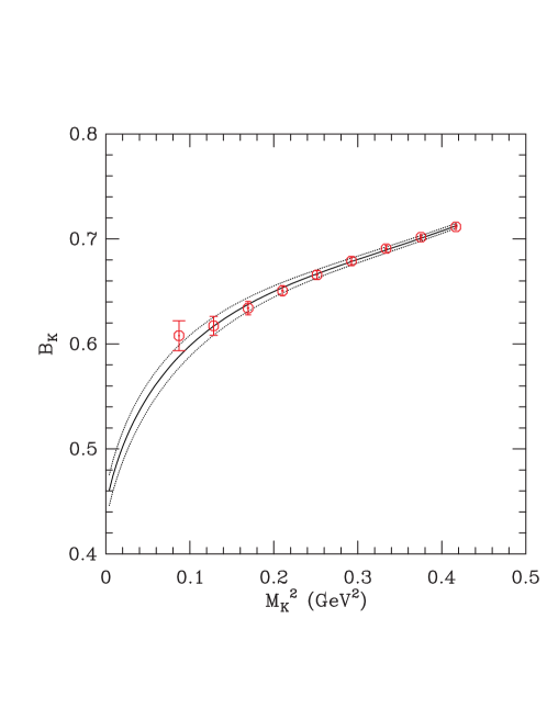
Figure 1: $B_{K}$ versus $m_{K}^{2}$ for degenerate quark mass combinations ($m_{x}=m_{y}$)

In Fig. 1, we plot $B_{K}$ as a function of $M_{K}^{2}$ for degenerate valence quarks ($m_{x}=m_{y}$). We fit the data to the form in eq. 8, with the cut-off scale chosen to be $\Lambda=4\pi f$. The fitting results are summarized in Table 2. The $\chi^{2}$ is rather high, considering that the data are correlated and we do not include the full covariance matrix. In particular, we observe that the curve does not fit the lightest data point very well.

One possible explanation for the mismatch as small quark mass is that it is due to taste-breaking in pion loops. As noted in Ref. [5], non-Goldstone pions dominate the loop contributions which lead to curvature at small $m_{K}^{2}$, and this reduces the expected curvature away from the continuum limit. This prediction is qualitatively consistent with what we observe. However, this behavior could also due to the finiteness of the volume, which also becomes important only for small $m_{K}^{2}$. Clearly this needs further investigation.

3 $B_{K}$ for non-degenerate quarks ($m_{x}\neq m_{y}$)

A more stringent test of the applicability of chiral perturbation theory is provided using non-degenerate quarks. The continuum prediction is [5]

$$B_{K} = c_{1}\bigg{(}1+\frac{1}{48\pi^{2}f^{2}}\Big{[}I_{\rm conn}+I_{\rm disc}\Big{]}\bigg{)}+c_{2}m_{xy}^{2}+c_{3}\frac{(m_{X}^{2}-m_{Y}^{2})^{2}}{m_{xy}^{2}}+c_{4}m_{xy}^{4}$$ (13)

The contribution from quark-connected diagrams is

$$I_{\rm conn} = 6m_{xy}^{2}\tilde{l}(m_{xy}^{2})-3l(m_{X}^{2})\Big{(}1+\frac{m_{X}^{2}}{m_{xy}^{2}}\Big{)}-3l(m_{Y}^{2})\Big{(}1+\frac{m_{Y}^{2}}{m_{xy}^{2}}\Big{)}\,,$$ (14)

while that from diagrams involving a hairpin vertex is

$$I_{\rm disc} = (I_{X}+I_{Y}+I_{\eta})/m_{xy}^{2}$$ (15)

$$I_{X} = \tilde{l}(m_{X}^{2})\frac{(m_{xy}^{2}+m_{X}^{2})(m_{U}^{2}-m_{X}^{2})(m_{S}^{2}-m_{X}^{2})}{m_{\eta}^{2}-m_{X}^{2}}-l(m_{X}^{2})\frac{(m_{xy}^{2}+m_{X}^{2})(m_{U}^{2}-m_{X}^{2})(m_{S}^{2}-m_{X}^{2})}{(m_{\eta}^{2}-m_{X}^{2})^{2}}$$ (16)

$$-l(m_{X}^{2})\frac{2(m_{xy}^{2}+m_{X}^{2})(m_{U}^{2}-m_{X}^{2})(m_{S}^{2}-m_{X}^{2})}{(m_{Y}^{2}-m_{X}^{2})(m_{\eta}^{2}-m_{X}^{2})}$$

$$-l(m_{X}^{2})\frac{(m_{U}^{2}-m_{X}^{2})(m_{S}^{2}-m_{X}^{2})-(m_{xy}^{2}+m_{X}^{2})(m_{S}^{2}-m_{X}^{2})-(m_{xy}^{2}+m_{X}^{2})(m_{U}^{2}-m_{X}^{2})}{m_{\eta}^{2}-m_{X}^{2}}$$

$$I_{Y} = I_{X}(m_{X}^{2}\leftrightarrow m_{Y}^{2})$$ (17)

$$I_{\eta} = l(m_{\eta}^{2})\frac{(m_{X}^{2}-m_{Y}^{2})^{2}(m_{xy}^{2}+m_{\eta}^{2})(m_{U}^{2}-m_{\eta}^{2})(m_{S}^{2}-m_{\eta}^{2})}{(m_{X}^{2}-m_{\eta}^{2})^{2}(m_{Y}^{2}-m_{\eta}^{2})^{2}}\,.$$ (18)

parameters	unit	average	error
$c_{1}$	1	0.4422	0.0145
$c_{2}$	$GeV^{-2}$	$-$1.4616	0.1611
$c_{3}$	$GeV^{-2}$	$-$	$-$
$c_{4}$	$GeV^{-4}$	1.4674	0.1913
$\chi^{2}$/d.o.f.	1	0.5396	0.3

Table 2: Fitting results of $B_{K}$ for degenerate quark mass combinations ($m_{x}=m_{y}$)

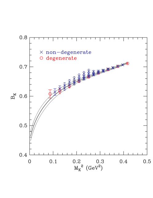
Figure 2: $B_{K}$ versus $m_{K}^{2}$ for both degenerate and non-degenerate quark mass combinations. The fit line is for the degenerate combinations only.

In Fig. 2, we plot $B_{K}$ data as a function of $M_{K}^{2}$, including data for both degenerate and non-degenerate valence quarks. We fit the data to the form in eq. 13. The results of the fit are summarized in Table 3.

When we compare Table 3 with Table 2, we observe the following: (1) $\chi^{2}/{\rm d.o.f.}$ is much smaller when we include non-degenerate combinations; (2) the low energy constants $c_{1}$, $c_{2}$ and $c_{4}$ are consistent within statistical uncertainty between the two fits; and (3) for our choice of the cut-off scale, $\Lambda=4\pi f$, the low energy constant $c_{3}$ is negligibly small. This comparison tells us that, for this cut-off, the effect of non-degenerate quark masses are dominated by the chiral logarithmic terms contained in $I_{\rm conn}$ and $I_{\rm disc}$, whereas the $c_{3}$ term plays no role. Overall, we learn that, while we can in principle determine $c_{1}$, $c_{2}$ and $c_{4}$ from the degenerate combinations alone, we have more confidence in the result when we include non-degenerate combinations. Furthermore, if we are to include higher order terms in chiral perturbation theory, as might be required at the heavier quark masses, the additional non-degenerate points will be essential.

The primary reason to study non-degenerate valence quarks is in order to extrapolate to the physical kaon, in which the non-degeneracy is almost maximal. The data shows a systematic increase in $B_{K}$ with increasing non-degeneracy. This effect is statistically significant though numerically small. When we have a satisfactory description of our data we will be able to extrapolate to the physical kaon mass.

4 Staggered chiral perturbation theory

A shortcoming with our present analysis is that it assumes that Goldstone and non-Goldstone pions are degenerate. We know, however, that taste symmetry is broken at ${\cal O}(a^{2})$, leading to splittings between pions with different tastes. A systematic way to incorporate such ${\cal O}(a^{2})$ effects is provided by staggered chiral perturbation theory [6, 7]. In the case of $B_{K}$, Van de Water and Sharpe have determined the next-to-leading-order (NLO) prediction of staggered chiral perturbation theory [5]. (In fact, a small modification of this result is necessary to describe our data, since we are using a mixed action.) Unfortunately, the result contains 21 unknown low energy constants, even at a single lattice spacing, and these must, at present, be determined from a fit to the lattice data. (Some can be determined in the future by calculating other matrix elements, or using non-perturbative renormalization to determine matching factors.) This is why we have chosen so many mass combinations (45 at present).

The fitting is further constrained if we know the masses of the non-Goldstone pions. These enter into loops, and, as noted above, lead to a modification of the curvature at small $m_{K}^{2}$. Because of this, in a companion work, we are calculating all pion masses (as well as those of other hadrons) using HYP-smeared valence staggered fermions [1]. A striking result of that study is that the taste-breaking effects are very small, much smaller than those with AsqTad improved staggered fermions. Thus it may be that we can get away with a continuum-like fit except at the smallest quark masses.

An exception to this comment concerns the contributions from quark-disconnected diagrams involving hairpin vertices. These bring in taste-singlet pions composed of (AsqTad) sea-quarks, for which ${\cal}(a^{2})$ terms are known to be large. Fortunately, the masses of these pions are available from the MILC collaboration studies.

As always when doing chiral extrapolations, it is important to push to as light a quark mass as possible (within the constraints of finite volume effects and computer time). In particular, this allows one to more thoroughly test the applicability of chiral perturbation theory at the order we work. Because of this, and to provide more data for fitting, we are presently extending the calculation to a lighter valence quark mass ($m=0.005$), which will also increase the total number of mass combinations to 55.

parameters	unit	average	error
$c_{1}$	1	0.4451	0.0149
$c_{2}$	$GeV^{-2}$	$-$1.5049	0.1672
$c_{3}$	$GeV^{-2}$	0.0305	0.0083
$c_{4}$	$GeV^{-4}$	1.5366	0.2021
$\chi^{2}$/d.o.f.	1	0.1888	0.0935

Table 3: Fitting results of $B_{K}$ for non-degenerate quark mass combinations ($m_{x}\neq m_{y}$)

5 Acknowledgment

W. Lee acknowledges with gratitude that the research at Seoul National University is supported by the KOSEF grant (R01-2003-000-10229-0), by the KOSEF grant of international cooperative research program, by the BK21 program, and by the US DOE SciDAC-2 program. S. Sharpe is supported in part by US DOE grant DE-FG02-96ER40956 and by the US DOE SciDAC-2 program.

References

- [1] T. Bae et al., Pion spectrum using improved staggered fermions, PoS LAT2006 (2006) 166, [hep-lat/0610056].
- [2] W. Lee and S. Sharpe, One-loop Matching coefficients for improved staggered bilinears, Phys. Rev. D66 (2002) 114501, [hep-lat/0208018].
- [3] Weonjong Lee, Progress in Kaon Physics on the Lattice, PoS LAT2006 (2006) 015, [hep-lat/0610058].
- [4] J. Kim et al., Calculating using a mixed action, PoS LAT2005 (2006) 338, [hep-lat/0510007]; T. Bae et al., Non-degenerate quark mass effect on with a mixed action, PoS LAT2005 (2006) 335, [hep-lat/0510008].
- [5] Ruth Van de Water and Stephen Sharpe, in Staggered Chiral Perturbation Theory , Phys. Rev. D73 (2006) 014003, [hep-lat/0507012].
- [6] Weonjong Lee and Stephen Sharpe, Partial Flavor Symmetry Restoration for Chiral Staggered Fermions, Phys. Rev. D60 (1999) 094503, [hep-lat/9905023].
- [7] C. Aubin and C. Bernard, Pion and kaon masses in staggered chiral perturbation theory, Phys. Rev. D68 (2003) 034014, [hep-lat/0304014].