Progress in Kaon Physics on the Lattice

Abstract:

We review recent progress in calculating kaon spectrum, pseudoscalar meson decay constants, $B_{K}$, $\epsilon^{\prime}/\epsilon$, $K\rightarrow\pi\pi$ matrix elements, kaon semileptonic form factors, and moments of kaon distribution amplitudes on the lattice. We also address the issue of how best to improve the staggered fermion formulation for the action and operators.

1 Introduction

Kaon physics is a rich resource when searching for new physics beyond the standard model. There have been a series of essential quantum jumps in the understanding of kaon spectrum, kaon decays, kaon mixing, partonic analysis of kaon, kaon form factors, and so on. In this article, we will review some of the recent progress in kaon physics.

First, we review recent progress in understanding the pattern of taste symmetry breaking in the pion multiplet spectrum of staggered fermions. We compare a number of popular improvement schemes for staggered fermions and provide a guide to the best scheme by comparing the mass splittings of the pion multiplet in various improvement schemes.

Second, we address the issue of calculating $f_{\pi}$ and $f_{K}$ with extremely high precision, which have a massive impact in determining some of the low energy constants such as $L_{5}$ and the CKM matrix elements. We review the results of MILC (AsqTad staggered fermions in $2+1$ flavor QCD), RBC/UKQCD (domain wall fermions in $2+1$ flavor QCD), and NPLQCD (a mixed action scheme in $2+1$ flavor QCD).

Third, we review the phenomenological importance of indirect CP violation for the CKM unitarity triangle. We review the history of calculating $B_{K}$ in quenched QCD, and compare the capabilities of the various improvement schemes for staggered fermions to reduce scaling violations in $B_{K}$. This comparison will guide us to the best scheme to improve staggered fermions. We will also review recent progress in calculating $B_{K}$ in $2+1$ flavor QCD using improved staggered fermions and domain wall fermions.

Fourth, we address critical issues in calculating $\epsilon^{\prime}/\epsilon$ on the lattice. We explain a serious ambiguity in defining a lattice version of left-right QCD penguin operators, in particular $Q_{6}$, which was originally pointed out by Golterman and Pallante. We review a recent numerical study on this issue by RBC, which confirms the original prediction by Golterman and Peris. This leads to a conclusive claim that it is not possible to reliably calculate the leading contribution of $Q_{6}$ to $\epsilon^{\prime}/\epsilon$ in quenched QCD. In addition, we also review theoretical progress in understanding the left-left QCD penguin operators by Golterman and Pallante. This explains the existence of another serious ambiguity in a lattice version of left-left QCD penguin operators, in particular $Q_{1}$, $Q_{2}$ and $Q_{4}$, which leads to the conclusion that it is not possible to reliably calculate even the sub-leading contribution of $Q_{4}$ to $\epsilon^{\prime}/\epsilon$ in quenched QCD. We also propose a solution to the problems in the end.

Fifth, we review the history of calculating the hadronic matrix elements of $K\rightarrow\pi\pi$ directly. We discuss the Maiani Testa no-go theorem, and consider a number of methods to get around it: the diagonalization method, the H parity boundary condition method, and the moving frame method. We also present recent numerical work in the moving frame by RBC.

Sixth, we review the progress in calculating the vector form factor of $K_{l3}$ decays on the lattice, which determines $|V_{us}|$ with high accuracy. The results of RBC, HPQCD/FNAL, and JLQCD are presented.

Seventh, we review the progress in calculating the first moment of the kaon distribution amplitude. The results of UKQCD and QCDSF/UKQCD are presented.

Finally, we summarize the whole discussion and end with some conclusions. In the final remarks, we propose to use $\overline{\rm Fat7}$ staggered fermions as the best candidate to generate $2+1$ unquenched gauge configurations using the rational hybrid Monte Carlo algorithm (RHMC).

2 Pion, Kaon spectrum

Staggered fermions have four degenerate tastes by construction, which leads to SU(4) taste symmetry in the continuum limit $a\to 0$. However, the taste symmetry is broken at a finite lattice spacing ($a>0$). The splittings in the pion multiplet spectrum are a non-perturbative measure of the taste symmetry breaking. From a theoretical point of view, a natural tool to study the pion multiplet spectrum is staggered chiral perturbation theory [1, 2]. According to staggered chiral perturbation theory, the taste symmetry breaking in pion multiplet spectrum happens in two steps: at ${\cal O}(a^{2})\approx{\cal O}(p^{2})$ the SU(4) taste symmetry is broken down to SO(4) taste symmetry, and at higher order of ${\cal O}(a^{2}p^{2})$ the SO(4) taste symmetry is broken down to the discrete spin-taste symmetry $SW_{4}$ [1]. As a consequence, we expect that, at ${\cal O}(a^{2})\approx{\cal O}(p^{2})$, the pion spectra can be classified into 5 irreducible representations of SO(4) taste symmetry: $\{\gamma_{5}\otimes I\}$, $\{\gamma_{5}\otimes\xi_{5}\}$, $\{\gamma_{5}\otimes\xi_{\mu}\}$, $\{\gamma_{5}\otimes\xi_{\mu 5}\}$, $\{\gamma_{5}\otimes\xi_{\mu\nu}\}$. The pion with $\xi_{5}$ taste is the Goldstone mode corresponding to a conserved axial symmetry which is broken spontaneously.

The splittings between pion multiplets reflect the taste symmetry breaking directly. As we improve the staggered fermion action and operators more, the splittings get smaller and the taste symmetry gets closer to SU(4). In other words, the splittings between pion multiplets can be used as a non-perturbative probe to measure how much of the taste symmetry is restored.

There have been a number of proposals to improve staggered fermions: Fat7 [3], AsqTad [3], HYP [4], $\overline{\rm Fat7}$ [5], and others. Unimproved staggered fermions have three serious problems: (1) large scaling violation, (2) large one-loop perturbative correction, and (3) large taste symmetry breaking, which are well established through a number of elaborate numerical studies. It turns out that HYP and $\overline{\rm Fat7}$ improvement schemes have the smallest one loop corrections ($\ll 5$ %) to bilinear operators [6], which resolves the problem of large perturbative corrections completely. The AsqTad and HYP improvement schemes are already being used extensively for numerical study of various physical observables, and it is important to determine which scheme is the best. Even though the perturbative comparison in Ref. [6] provides a hint that HYP and $\overline{\rm Fat7}$ schemes are better than the AsqTad scheme, it was not conclusive at that time due to a lack of non-perturbative evidence of improvement for the remaining two issues. In this context, it is quite important to compare the size of splittings between pion multiplets for various improvement schemes, which will tell us which improvement scheme is best to restore the SU(4) taste symmetry. We will address the issue of large scaling violation later when we talk about $B_{K}$. Here, let us focus on the issue of the taste symmetry breaking by looking into splittings among pion multiplets.

In order to probe the size of the taste symmetry breaking for unimproved staggered fermions, we have calculated the pion multiplet spectrum in quenched QCD ($\beta=6.0$ and $16^{3}\times 64$ lattice) and preliminary results are presented in Ref. [7]. In Fig. 1, we show $(am_{\pi})^{2}$ as a function of quark mass $am_{q}$ for various pion multiplets. As discussed in Ref. [7], there are two independent methods to construct the bilinear operators using staggered fermions: (1) the Kluberg-Stern method and (2) the Golterman method. In Fig. 1, the left (right) plot is obtained using the Kluberg-Stern (Golterman) method. Note that there is essentially no difference between the Kluberg-Stern and Golterman methods. We also observe that the splittings among pion multiplets are comparable to the light pion masses, which implies that ${\cal O}(a^{2})\approx{\cal O}(p^{2})$. In addition, note that the slopes are noticeably different for various tastes, which implies that ${\cal O}(a^{2}p^{2})$ terms are so large as to be noticeable in the case of unimproved staggered fermions, even though they are of higher order in staggered chiral perturbation theory.

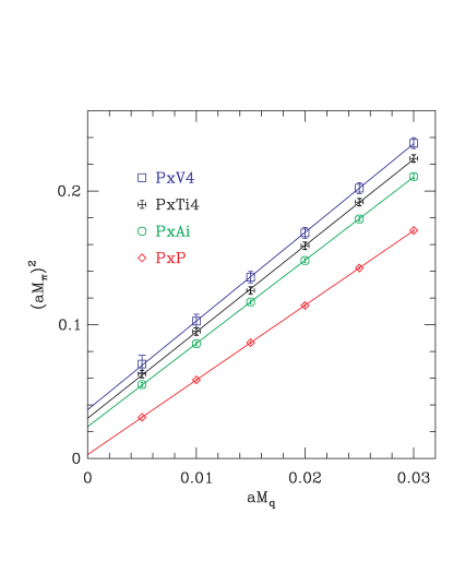
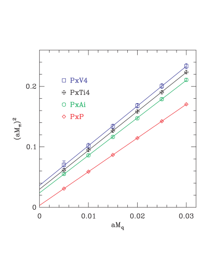
Figure 1: $(am_{\pi})^{2}$ vs. $am_{q}$ for unimproved staggered fermions: (left) using the Kluberg-Stern method; (right) using the Golterman method.

In Fig. 2, we compare the results of AsqTad staggered fermions with those of HYP staggered fermions. The AsqTad staggered fermion data comes originally from Ref. [8] whereas the HYP staggered fermion data comes from Ref. [7]. Since AsqTad staggered fermions use a Symanzik improved gauge action with $a=0.12$fm and HYP staggered fermions use the unimproved Wilson plaquette action with $a=0.1$fm, we expect that the scaling violations associated with the background gauge configurations are similar in both cases. In the case of AsqTad staggered fermions, the size of the taste symmetry breaking effect is comparable to the light pion masses, which implies that ${\cal O}(a^{2})\approx{\cal O}(p^{2})$. In addition, note that the slopes of pion multiplets with different tastes are the same, which implies that the ${\cal O}(a^{2}p^{2})$ terms are negligibly small for AsqTad staggered fermions.

In the right-hand side of Fig. 2, we show data for HYP staggered fermions. In this plot, we observe two things. First, the splitting among pion multiplets are extremely suppressed within $2\sigma$ of the data point error bar, which implies that ${\cal O}(a^{2})\ll{\cal O}(p^{2})$. Second, we notice that the slopes of pion multiplets with different tastes coincide within statistical uncertainty, which implies that the ${\cal O}(a^{2}p^{2})$ terms are so small that the effect is not detected at all.

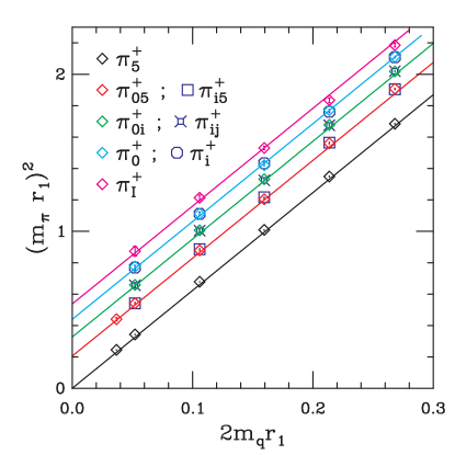
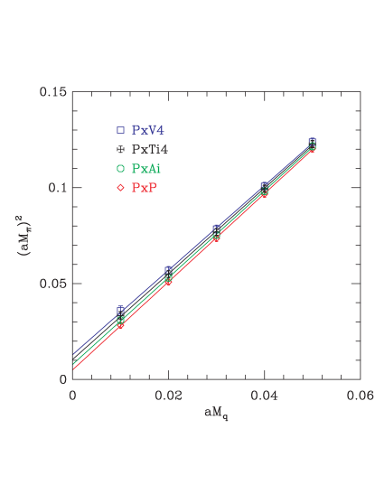
Figure 2: $(am_{\pi})^{2}$ vs. $am_{q}$: (left) for AsqTad staggered fermions; (right) for HYP staggered fermions (using the Golterman method).

Therefore, from Fig. 2, we conclude that HYP staggered fermions are remarkably better than AsqTad staggered fermions with regards to reducing the taste symmetry breaking effect. From Fig. 1 and Fig. 2, the ${\cal O}(a^{2}p^{2})$ terms are so large for unimproved staggered fermions that the effect was noticeable in the data, whereas these higher order terms are negligibly small in the case of AsqTad and HYP staggered fermions, which we can count as a big improvement. Therefore, we can rank the improvement efficiency of various staggered fermions with regards to taste symmetry restoration as follows:

$$\mbox{unimproved stag}<\mbox{AsqTad stag}<\mbox{HYP stag}$$ (1)

More details on the comparison of various improvement schemes can be found in Ref. [7].

3 $f_{\pi}$ and $f_{K}$

A precise determination of low energy constants in QCD is one of the major goals that we want to achieve on the lattice. In particular, $f_{\pi}$ and $f_{K}$ are relatively cheap to calculate on the lattice and their analysis is straight forward. The real challenge is that we need to produce a large ensemble of gauge configurations which includes sea quark back-reaction (sea quark determinant) with $N_{F}=2+1$ flavors ($m_{u}=m_{d}\neq m_{s}$). This procedure is quite expensive computationally. Then, we compute valence quark propagators on the gluon backgrounds to calculate hadron spectrum and hadronic matrix elements. To get as much physics information as possible from the valuable gauge configurations with specific sea quark masses, we use many values of valence quark masses, i.e. not just the same values as the sea quark masses. This physical set-up is known as “partially quenched QCD”. It has been studied with a number of lattice fermion formulations: (1) AsqTad staggered fermions, (2) Wilson clover fermions, (3) Wilson twisted mass fermions, (4) domain wall fermions, and (5) overlap fermions. In the following, we discuss the cases of AsqTad staggered fermions, domain wall fermions, and a mixed action approach (valence quarks are domain wall fermions and sea quarks are AsqTad staggered fermions).

3.1 $f_{\pi}$ and $f_{K}$ using AsqTad staggered fermions

Staggered fermions are fastest to simulate on the lattice, and have an exact axial symmetry which protects the quark mass from additive renormalization and makes it possible to calculate weak matrix elements reliably. The physical quark flavors are each represented by a staggered fermion field, so for three quark flavors there is an exact SU(3) flavor symmetry (when the quark masses are degenerate) as in the continuum, along with SU(4) taste symmetry of each of the staggered fermion fields (which is broken at finite lattice spacing but restored in the continuum limit). The hadronic operators can be taken to have a specific taste, so the lattice formulation with staggered fermions reproduces the continuum one at tree level in chiral perturbation theory. However, pions with all kinds of tastes appear in loops, and through this taste violations enter everywhere. Hence, it is necessary to take into account taste violations (directly related to discretization effects) within chiral perturbation theory in order to fit the data and extract physical information with high precision. A systematic tool to incorporate taste violations into the data analysis is the staggered chiral perturbation theory [1, 2].

Another caveat regarding broken taste symmetry is that we take $\sqrt[4]{{\rm Det}(D+m)}$ as the fermion determinant to get a single taste per sea quark flavor. This is often called the “fourth-root trick”. There is a possibility that $\sqrt[4]{{\rm Det}(D+m)}$ produces non-perturbatively violations of locality and universality in the continuum limit, which might cause staggered fermions not to reproduce QCD. However, recent arguments and numerical investigations give encouraging indications that this possibility does not occur. For more details on this issue, see Ref. [10].

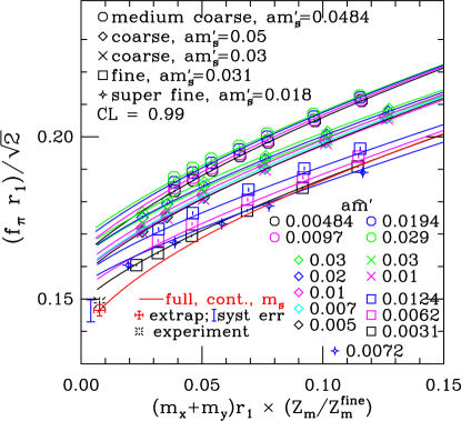
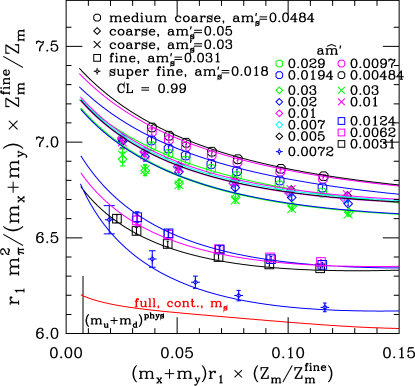
Figure 3: $f_{\pi}$ vs. $m_{x}+m_{y}$ (left) and $m_{\pi}^{2}/(m_{x}+m_{y})$ vs. $m_{x}+m_{y}$ (right). The data are obtained using AsqTad staggered fermions in $N_{F}=2+1$ partially quenched QCD.

Recently, MILC has been generating dynamical gauge configurations with $N_{F}=2+1$ flavor sea quarks (AsqTad staggered fermions). These configurations include coarser lattices ($a=0.15$fm), coarse lattices ($a=0.12$fm), fine lattices ($a=0.09$fm) and super-fine lattices ($a=0.06$fm). On these lattices, the strange sea quark mass ($M_{s}$) of simulation runs the range of $0.7m_{s}\lesssim M_{s}\lesssim 1.2m_{s}$. The light sea quark mass of simulation goes down to $m_{u}=m_{d}\approx 11$ MeV ($m_{\pi}\approx 240$ MeV). The physical volumes of the lattices range from $(2.4fm)^{3}$ to $(3.4fm)^{3}$. Using these gauge configurations, MILC has been calculating full pion multiplet spectrum and decay constants for the Goldstone pions and kaons. The results are presented in Fig. 3. In this extensive calculation, MILC concentrates on the analysis of masses and decay constants of Goldstone pions and kaons. This analysis also involves the masses of non-Goldstone pions and kaons; these enter in one-loop chiral logs at NLO in staggered chiral perturbation theory [11]. In the data analysis, it is necessary to cut out the data points of heavier quark masses one by one in order to get good fits to the form suggested by staggered chiral perturbation theory. The most updated results are summarized in Table 1. For more details, see Ref. [9].

observable	value
$f_{\pi}$	$128.6\pm 0.4\pm 3.0$ MeV
$f_{K}$	$155.3\pm 0.4\pm 3.1$ MeV
$f_{K}/f_{\pi}$	$1.208(2)_{-14}^{+7}$
$V_{us}$	$0.2223_{-14}^{+26}$
$m_{s}(2{\rm GeV},\overline{\rm MS})$	90(0)(5)(4)(0) MeV
$m_{u,d}(2{\rm GeV},\overline{\rm MS})$	3.3(0)(2)(2)(0) MeV
$m_{s}/m_{u,d}$	27.2(0)(4)(0)(0)
$L_{5}$	$2.0(3)(2)\times 10^{-3}$

Table 1: Results of data analysis by MILC.

3.2 $f_{\pi}$ and $f_{K}$ using domain wall fermions

In the domain wall fermion formulation, the breaking of chiral symmetry is due only to the finite length of the 5th dimension, which allows a small additive renormalization to quark masses. We call this a “residual quark mass”; it is typically only a few MeV and hence under control. Domain wall fermions are computationally typically two orders of magnitude more expensive than improved staggered fermions. Since we can use continuum chiral perturbation theory for the analysis of domain wall fermion data, the theoretical interpretation is simpler and more straightforward compared to improved staggered fermions.

parameter	value
lattice	$16^{3}\times 32$ and $24^{3}\times 64$
$L_{s}$	16
$aM_{5}$	1.8
$a$	0.125 fm
$am_{s}$	0.04
$am_{u,d}$	0.01, 0.02, 0.03

Table 2: Parameters of dynamical domain wall fermion simulation by RBC and UKQCD.

The RBC and UKQCD collaborations use domain wall fermions with Iwasaki gluon action to generate dynamical gauge configurations with $N_{F}=2+1$ sea quark flavors. The simulation parameters are summarized in Table 2. These lattices are comparable with the coarse MILC lattices ($a=0.12$ fm). These groups measured pion decay constants and pion spectra in partially quenched QCD, and the preliminary results are shown in Fig. 4. They put elaborate effort into fitting the data of $f_{\pi}$ and $m_{\pi}^{2}/m_{q}$ simultaneously to the NLO form suggested by partially quenched chiral perturbation theory. It turns out that the simultaneous fits fail to describe the data. They believe that this failure is due to the fact that the quark masses are too heavy to interpret the data based on chiral perturbation theory. For more details, see Ref. [14].

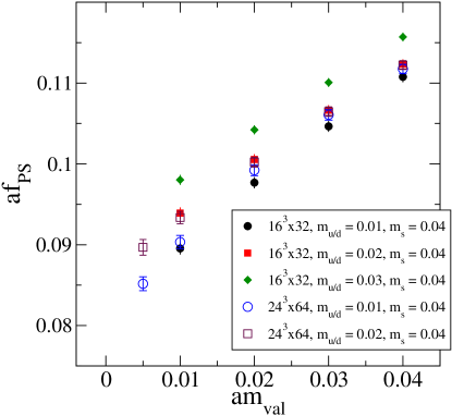
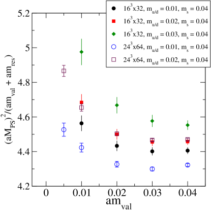
Figure 4: $af_{\pi}$ vs. $am_{\rm val}$ (left) and $(am_{\pi})^{2}/(m_{\rm val}+m_{\rm res})$ vs. $m_{\rm val}$ (right). The data were obtained using domain wall fermions in $N_{F}=2+1$ partially quenched QCD.

3.3 $f_{K}/f_{\pi}$ using a mixed action scheme

Another possibility in partially quenched QCD is to use a mixed action scheme. This is the approach taken by the LHPC and NPLQCD collaborations [12]. In this approach, the sea quarks are AsqTad staggered fermions and the valence quarks are domain wall fermions. Specifically, they do HYP smearing over the MILC gauge configurations with $N_{F}=2+1$ AsqTad staggered sea quarks and calculate the valence quark propagators using domain wall fermions over these configurations to measure $f_{K}/f_{\pi}$. In this approach, the valence quark masses are tuned such that the pion masses match the Goldstone pion masses of AsqTad sea quarks.

In the continuum SU(3) chiral perturbation theory, one can show that $f_{K}/f_{\pi}$ is given, at the next-to-leading (NLO) order, by

$$\frac{f_{K}}{f_{\pi}} = 1+\chi_{\log}+8yL_{5}(\mu)$$ (2)

$$y = \frac{m_{K}^{2}-m_{\pi}^{2}}{f_{\pi}^{2}}$$ (3)

$$L_{5}(f^{0}_{\pi}) = L_{5}(\mu)-\frac{3}{8}\frac{1}{16\pi^{2}}\log(f^{0}_{\pi}/\mu)$$ (4)

where $\mu$ is a renormalization scale in chiral perturbation theory, $\chi_{\log}$ represents all the NLO chiral log corrections collectively, and $f^{0}_{\pi}$ is the physical value of pion decay constant. In Fig. 5, we show $L_{5}(f^{0}_{\pi})$ calculated using the mixed action scheme. It is interesting to note that the final value of $f_{K}/f_{\pi}$ obtained by NPLQCD is consistent with MILC, even though they apply the continuum chiral perturbation theory to analyze data of the mixed action scheme. For more details, see Ref. [12].

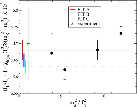
Figure 5: $L_{5}(f^{0}_{\pi})$ vs. $m_{\pi}^{2}/f_{\pi}^{2}$ calculated by NPLQCD, using a mixed action scheme.

4 Indirect CP violation and $B_{K}$

In nature, there are two kinds of CP violations in the neutral kaon system: indirect CP violation and direct CP violation. The neutral kaon states in nature are described as CP eigenstates with a tiny impurity which is parametrized as $\epsilon$. In experiment, $\epsilon$ is determined precisely as follows:

$$\epsilon=(2.280\pm 0.013)\times 10^{-3}\times\exp(i\pi/4)$$ (5)

From the standard model, it is possible to express $\epsilon$ in terms of $K^{0}-\bar{K}^{0}$ mixing as follows [13]:

$$\epsilon = C_{\epsilon}\ \exp(i\pi/4)\ {\rm Im}\lambda_{t}\ X\ \hat{B}_{K}$$ (6)

$$X = {\rm Re}\lambda_{c}[\eta_{1}S_{0}(x_{c})-\eta_{3}S_{3}(x_{c},x_{t})]-{\rm Re}\lambda_{t}\eta_{2}S_{0}(x_{t})$$ (7)

$$\lambda_{i} = V_{is}^{*}V_{id},\qquad x_{i}=m_{i}^{2}/M_{W}^{2}$$ (8)

$$C_{\epsilon} = \frac{G_{F}^{2}f_{K}^{2}m_{K}M_{W}^{2}}{6\sqrt{2}\pi^{2}\Delta m_{K}}$$ (9)

Here, note that $S_{i}$ (the Inami-Nam functions) and $\eta_{i}$ are determined reliably from perturbation theory; they represent the remaining effect of heavy particles when they are integrated out. The kaon bag parameter $\hat{B}_{K}$ is defined as

$$B_{K} = \frac{\langle\bar{K}_{0}|[\bar{s}\gamma_{\mu}(1-\gamma_{5})d][\bar{s}\gamma_{\mu}(1-\gamma_{5})d]|K_{0}\rangle}{\frac{8}{3}\langle\bar{K}_{0}|\bar{s}\gamma_{\mu}\gamma_{5}d|0\rangle\langle 0|\bar{s}\gamma_{\mu}\gamma_{5}d|K_{0}\rangle}$$ (10)

$$\hat{B}_{K} = C(\mu)B_{K}(\mu)$$ (11)

$$C(\mu) = \alpha_{s}(\mu)^{-\frac{\gamma_{0}}{2\beta_{0}}}[1+\alpha_{s}(\mu)J_{3}]$$ (12)

where $\mu$ is a renormalization scale of the $\Delta S=2$ operator, and $\hat{B}_{K}$ is renormalization group invariant. $V_{ij}$ is the CKM matrix element of the standard model. The theoretical challenge is to calculate $B_{K}$ with such a high precision that it over-constrains the unitarity of the CKM matrix.

It is possible to determine $\hat{B}_{K}$ from the untarity triangle if we obtain the CKM matrix elements from other experimental results. In Fig. 6, we show the result of $\hat{B}_{K}$ determined from the unitarity triangle. The result reported in CKM 2005 is $\hat{B}_{K}=0.68\pm 0.10$.

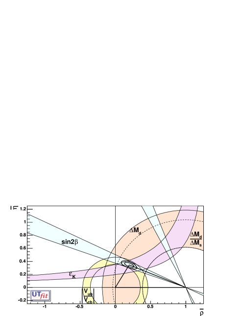
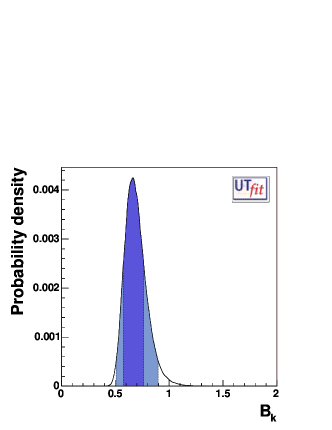
Figure 6: $\hat{B}_{K}$ determined from the unitarity triangle.

4.1 $B_{K}$ in quenched QCD

There have been a number of efforts to calculate $B_{K}$ in quenched QCD using staggered fermions [15, 16], twisted mass (TM) Wilson fermions [17], domain wall fermions [18, 19], and overlap fermions [20, 21]. In Fig. 7, the results of these calculations are summarized. We observe a large scaling violation in the calculation of $B_{K}$ using unimproved staggered fermions by JLQCD [15]. However, it is possible to reduce the scaling violation down to a negligibly small level using the HYP improvement scheme to improve the staggered fermion action and operators [16]. We will address the issue of scaling violation in detail in Sec. 4.2. An interesting demonstration of the progress in $B_{K}$ calculations is that the value of $B_{K}$ calculated using the TM Wilson fermions ends up being in agreement with other $B_{K}$ calculations using different fermion formulations [17]. The calculation of $B_{K}$ with TM Wilson fermions has been discussed in great detail in the plenary talk by Pena [22] so we skip all the details here. The values of $B_{K}$ calculated by CP-PACS [18] and by RBC [19] using domain wall fermions are in good agreement with those of other fermion formulations. The $B_{K}$ values calculated by two independent groups [20, 21] using overlap fermions are also in agreement with those of other fermion formulations, although they have relatively large error bars.

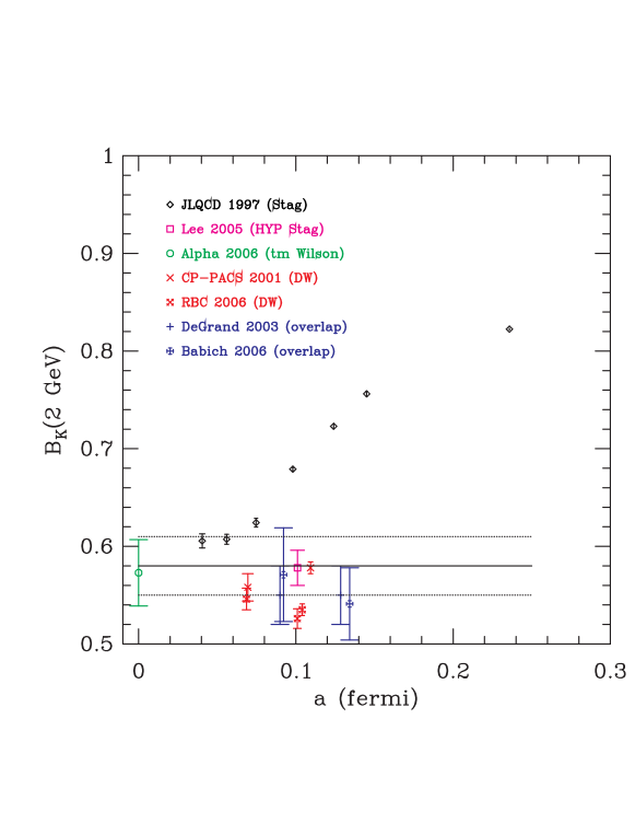
Figure 7: $B_{K}(2GeV,{\rm NDR})$ calculated in quenched QCD.

In these calculations, it is assumed that $m_{s}=m_{d}$, i.e. the effects of non-degenerate quark masses are neglected. A simple-minded world average estimate of quenched $B_{K}$ with degenerate quarks is $B_{K}(2{\rm GeV},{\rm NDR})=0.58(4)$.

4.2 Scaling violation in $B_{K}$ and its reduction with improved staggered fermions

We now focus on the scaling violation in $B_{K}$ calculated using staggered fermions. In Fig. 8, we show $B_{K}$ data as a function of lattice spacing $a$ (fm). Here, we observe that there is a large scaling violation (= discretization error) in the data calculated by JLQCD using the unimproved staggered fermion action and unimproved operators (constructed using thin links). The blue (green) data points in Fig. 8 represent the $B_{K}$ values calculated using the AsqTad (HYP) staggered fermion action and unimproved operators [23]. We notice that in this case the scaling violations are reduced by about 50%. This comparison tells us that the HYP staggered fermion action is much more efficient in reducing the scaling violations than the AsqTad staggered fermion action. However, we also observe that the remaining scaling violations are still substantial. The red data points in Fig. 8 represents the $B_{K}$ values obtained using the HYP staggered fermion action and the improved operators with HYP fat links [16]. In this case, the $B_{K}$ value at $a=0.1$ fm is consistent with the world average which is obtained by extrapolation to the continuum limit of ($a=0$). This implies that, once we improve the staggered fermion action and operators with HYP fat links, the scaling violations in $B_{K}$ are reduced down to a negligibly small level.

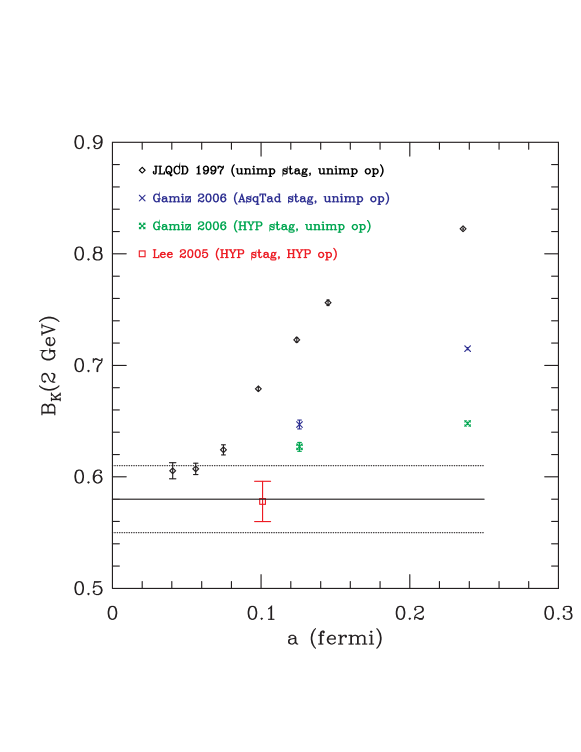
Figure 8: $B_{K}(2GeV,{\rm NDR})$ calculated using various staggered fermion formulations.

From Fig. 8, we conclude that we can rank the improvement efficiency of various staggered fermions with regards to reducing the scaling violations as follows:

$$\mbox{unimproved stag}<\mbox{AsqTad stag}<\mbox{HYP stag}$$ (13)

Combining this conclusion with that of Sec. 2, we see that HYP staggered fermions are remarkably better than AsqTad staggered fermions in reducing the taste symmetry breaking effect, the scaling violations, and the one-loop perturbative corrections simultaneously [6].

4.3 $B_{K}$ in unquenched QCD with $N_{F}=2+1$

Recently, there have been two serious attempts to calculate $B_{K}$ in unquenched QCD with $N_{F}=2+1$. In Fig. 9, we show $B_{K}$ data in $N_{F}=2+1$ flavor QCD. On the left-hand side of Fig. 9, we show the $B_{K}$ data of the RBC and UKQCD collaborations calculated using domain wall fermions at $a=0.125$ fm [24]. On the right-hand side of Fig. 9, we present the $B_{K}$ data ($a=0.12$ fm) obtained using a mixed action scheme in which valence quarks are HYP staggered fermions and sea quarks are AsqTad staggered fermions [25]. The $B_{K}$ data of domain wall fermions does not have a noticeable dependence on the non-degenerate quark masses. However, we observe that the $B_{K}$ data of improved staggered fermions shows a noticeable dependence on the non-degenerate quark masses, corresponding to about $3\sigma$ difference between the degenerate and non-degenerate quark mass combinations near the physical kaon mass. Certainly, this is a puzzle. One possible explanation is that there is a significant difference in statistics between the two sets of data: 75 measurements for the domain wall fermion data and 640 measurements for the improved staggered fermion data. In other words, it might be that this dependence on the non-degenerate masses only shows up with extremely high statistics. At any rate, this issue needs further investigation in the future.

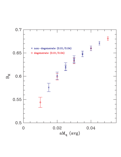
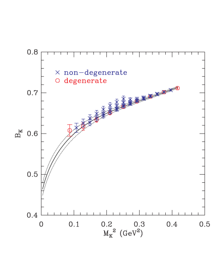
Figure 9: $B_{K}^{\rm bare}$ in unquenched QCD with $N_{F}=2+1$; (left) calculated by RBC and UKQCD collaborations using domain wall fermions and (right) calculated by Lee et al. using a mixed action scheme in which valence quarks are HYP staggered fermions and sea quarks are AsqTad staggered fermions.

There has been another attempt to calculate $B_{K}$ in unquenched QCD using the AsqTad staggered fermions and unimproved operators, where $B_{K}$ is calculated with degenerate quark masses set to $am_{s}/2$ [23]. Since this work does not address the main issue of this section, we omit the details.

5 Direct CP violation and ${\rm Re}(\epsilon^{\prime}/\epsilon)$

Direct CP violation occurs in kaon decays via electroweak interactions where the CP symmetry is explicitly broken. This process is parametrized by $\epsilon^{\prime}/\epsilon$. Recently the KTeV and NA48 collaborations have determined ${\rm Re}(\epsilon^{\prime}/\epsilon)$ from high statistics experiments [26, 27]. The results are

$${\rm Re}(\epsilon^{\prime}/\epsilon) = (20.7\pm 2.8)\times 10^{-4}\qquad\mbox{(KTeV)}$$ (14)

$$= (14.7\pm 2.2)\times 10^{-4}\qquad\mbox{(NA48)}$$ (15)

Here, note that both KTeV and NA48 claim that ${\rm Re}(\epsilon^{\prime}/\epsilon)$ is large and positive ($\gg 1.0\times 10^{-4}$).

From the standard model, we can derive the theoretical expression for $\epsilon^{\prime}/\epsilon$ as follows [13]:

$$\epsilon^{\prime}/\epsilon = {\rm Im}(V_{ts}^{*}V_{td})\Big{[}P^{(1/2)}-P^{(3/2)}\Big{]}\exp(i\Phi)$$ (16)

$$P^{(1/2)} = r\sum_{i=3}^{10}y_{i}(\mu)\langle Q_{i}(\mu)\rangle_{0}(1-\Omega_{\rm IB})$$ (17)

$$P^{(3/2)} = \frac{r}{\omega}\sum_{i=7}^{10}y_{i}(\mu)\langle Q_{i}(\mu)\rangle_{2}$$ (18)

$$\langle Q_{i}\rangle_{I} = \langle\pi\pi(I)|Q_{i}|K\rangle$$ (19)

$$r = \frac{G_{F}\omega}{2|\epsilon|{\rm Re}(A_{0})}$$ (20)

where $\mu$ is a renormalization scale of the $Q_{i}$ operators. Here, $P^{(1/2)}$ and $P^{(3/2)}$ represent the $\Delta I=1/2$ and $\Delta I=3/2$ contributions to $\epsilon^{\prime}/\epsilon$ respectively. The Wilson coefficient functions $y_{i}(\mu)$ can be determined reliably from the perturbation theory in a specific renormalization scheme. Note that the phase shift $\Phi=\Phi_{\epsilon^{\prime}}-\Phi_{\epsilon}\approx 0$ and $\omega=0.045$ (the $\Delta I=1/2$ rule). The parameter $\Omega_{\rm IB}$ represents the isospin breaking effect.

As can be seen in Eq. 16, $\epsilon^{\prime}/\epsilon$ is obtained as a result of destructive interferences between $P^{(1/2)}$ and $P^{(3/2)}$. In particular, $P^{(3/2)}$ is fully dominated by electroweak penguin contributions, especially $Q_{8}$. $P^{(1/2)}$ on the other hand is governed by QCD penguin contributions, especially $Q_{6}$. The main sources of uncertainty in the calculation of $\epsilon^{\prime}/\epsilon$ are the hadronic matrix elements $\langle\pi\pi(I)|Q_{i}|K\rangle$. Hence, the theoretical challenge on the lattice is to calculate $\langle\pi\pi(I)|Q_{i}|K\rangle$ reliably.

The RBC and CP-PACS collaborations reported that $\epsilon^{\prime}/\epsilon$ is small and negative. Their calculation is done in quenched QCD with operators defined in the SU(3) flavor group theory using domain wall fermions [28, 29]. However, Golterman and Pallante have pointed out that there is an serious ambiguity in the lattice version of left-right QCD penguin operators ($Q_{6}$ and $Q_{5}$) because the flavor group in quenched QCD is not SU(3) but SU(3—3) [30]. It turns out that the ambiguity in $Q_{6}$ has such a large effect on $\epsilon^{\prime}/\epsilon$ that it can flip the sign of $\epsilon^{\prime}/\epsilon$ in quenched QCD: this has been demonstrated in calculations using HYP staggered fermions [31, 32]. Recently, the RBC Collaboration have investigated this issue in great detail [33], which will be discussed in the next section. In addition, Golterman and Pallante point out that there is another ambiguity in $Q_{i}$ ($i=1,2,3,4$) in quenched QCD, which has a serious effect on ${\rm Re}(A_{0})$ and the sub-leading contribution of $Q_{4}$ on $\epsilon^{\prime}/\epsilon$ [34]. In other words, it is not possible to calculate reliably even the sub-leading contribution of $Q_{4}$ as well as the leading contribution of $Q_{6}$ to $\epsilon^{\prime}/\epsilon$ in quenched QCD. We will address this issue later.

5.1 Ambiguity in $Q_{6}$ and $Q_{5}$

We now focus on the left-right QCD penguin operators, especially $Q_{6}$ which makes the dominant contribution to $P^{(1/2)}$. In the standard model, $Q_{6}$ is defined as

$$Q_{6}=\bar{s}\gamma_{\mu}(1-\gamma_{5})d\sum_{q}\bar{q}\gamma_{\mu}(1+\gamma_{5})q$$ (21)

$Q_{6}$ belong to the (8,1) irreducible representation of the $SU(3)_{L}\otimes SU(3)_{R}$ flavor symmetry group. Unfortunately, $Q_{6}$ mixes with $\tilde{Q}_{i}$ ($i=3,4,5,6$) in (partially) quenched QCD, where for example, $\tilde{Q}_{6}$ is defined as

$$\tilde{Q}_{6}=\bar{s}\gamma_{\mu}(1-\gamma_{5})d\sum_{\tilde{q}}\bar{\tilde{q}}\gamma_{\mu}(1+\gamma_{5})\tilde{q}$$ (22)

where $\tilde{q}$ represents a ghost quark. Here, note that the flavor symmetry of (partially) quenched QCD is not $SU(3)$ but $SU(3+N_{F}|3)$ where $N_{F}$ is the number of sea quark flavors. In quenched QCD ($N_{F}=0$), Golterman and Pallante propose to decompose $Q_{6}$ as follows:

$$Q_{6} = Q_{6}^{QS}+Q_{6}^{QNS}$$ (23)

$$Q_{6}^{QS} = \frac{1}{2}\bar{s}\gamma_{\mu}(1-\gamma_{5})d\sum_{Q}\bar{Q}\gamma_{\mu}(1+\gamma_{5})Q$$ (24)

$$Q_{6}^{QNS} = \frac{1}{2}\bar{s}\gamma_{\mu}(1-\gamma_{5})d\sum_{Q}\bar{Q}\gamma_{\mu}(1+\gamma_{5})AQ$$ (25)

where $Q=(u,d,s,\tilde{u},\tilde{d},\tilde{s})$ and $A={\rm diag}(1,1,1,-1,-1,-1)$ is a diagonal matrix. See Ref. [30, 33] for the details of the group theoretical interpretation on this decomposition. $Q_{6}^{QS}$ can be represented by a set of operators in quenched chiral perturbation theory which have analogues in continuum chiral perturbation theory. However, $Q_{6}^{QNS}$ introduces a new low energy constant which is called $\alpha_{q}^{NS}$. In addition, Golterman and Peris have predicted that $\alpha_{q}^{NS}\approx 60\alpha_{q1}^{(8,1)}$ [35], which implies that the matrix elements of $Q_{6}$ are completely dominated by unphysical leading contribution from the lattice artifact $\alpha_{q}^{NS}$. Unfortunately, the work by the RBC and CP-PACS collaborations in Ref. [28, 29] contains this artifact as it is. As mentioned, the work of Ref. [31, 32] shows clearly that this ambiguity is so large that it can even flip the sign of $\epsilon^{\prime}/\epsilon$.

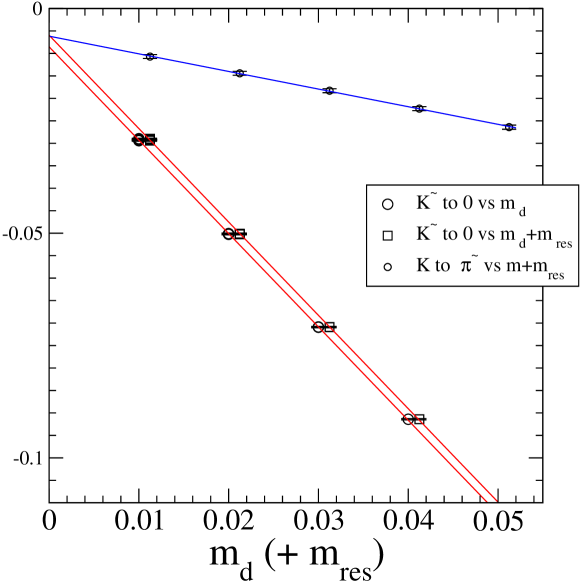
Figure 10: $\alpha_{q}^{NS}$ in quenched QCD calculated by the RBC collaboration.

Recently, the RBC collaboration has measured the low energy constant $\alpha_{q}^{NS}$ by two independent methods [33]: (1) using the hadron matrix element of $\tilde{K}\rightarrow 0$ which is originally suggested by Golterman and Pallante, and (2) using the $K^{+}\rightarrow\tilde{\pi}^{+}$ matrix element. In the case of domain wall fermions, the 2nd method has the advantage that one does not have to worry about the residual quark mass $m_{res}$, because the divergent NLO term vanishes in the limit of degenerate quark masses. In Fig. 10, we show the procedure to obtain $\alpha_{q}^{NS}$ by extrapolation to the chiral limit. The figure demonstrates that both methods produce the same result in the chiral limit and it is consistent with the prediction by Golterman and Peris. See Ref. [33] for more details.

5.2 Ambiguity in $Q_{3}$ and $Q_{4}$

Here, we focus on the left-left QCD penguin operators ($Q_{3}$, $Q_{4}$, part of $Q_{1}$ and $Q_{2}$, $\cdots$). As an example, let us consider $Q_{3}$ and $Q_{4}$:

$$Q_{3} = \bar{s}_{\alpha}\gamma_{\mu}(1-\gamma_{5})d_{\alpha}\sum_{q}\bar{q}_{\beta}\gamma_{\mu}(1-\gamma_{5})q_{\beta}=(\bar{s}_{\alpha}d_{\alpha})_{L}\sum_{q}(\bar{q}_{\beta}q_{\beta})_{L}$$ (27)

$$Q_{4} = \bar{s}_{\alpha}\gamma_{\mu}(1-\gamma_{5})d_{\beta}\sum_{q}\bar{q}_{\beta}\gamma_{\mu}(1-\gamma_{5})q_{\alpha}=(\bar{s}_{\alpha}d_{\beta})_{L}\sum_{q}(\bar{q}_{\beta}q_{\alpha})_{L}$$ (28)

Both $Q_{3}$ and $Q_{4}$ belong to the (8,1) irreducible representation of the $SU(3)_{L}\otimes SU(3)_{R}$ flavor symmetry group, which also corresponds to $I=1/2$. For the following discussion it is convenient to change the operator basis as follows:

$$Q_{\pm}=Q_{3}\pm Q_{4}$$ (29)

Here, note that $Q_{-}$ ($Q_{+}$) is symmetric (anti-symmetric) in the two anti-quark flavor indices and two quark flavor indices. Once more, the problem is that the flavor symmetry group of (partially) quenched QCD is not $SU(3)$ but $SU(3+N_{F}|3)$. Hence, $Q_{\pm}$ is reducible under $SU(3+N_{F}|3)$. We can decompose $Q_{\pm}$ as follows:

$$Q_{\pm} = \frac{3}{N_{F}}Q^{S}_{\pm}+Q^{A}_{\pm}$$ (30)

$$Q^{S}_{\pm} = (\bar{q}_{\alpha}\Lambda q_{\alpha})_{L}(\bar{q}_{\beta}q_{\beta})_{L}\pm(\bar{q}_{\alpha}\Lambda q_{\beta})_{L}(\bar{q}_{\beta}q_{\alpha})_{L}$$ (31)

$$Q^{A}_{\pm} = (\bar{q}_{\alpha}\Lambda q_{\alpha})_{L}(\bar{q}_{\beta}Aq_{\beta})_{L}\pm(\bar{q}_{\alpha}\Lambda q_{\beta})_{L}(\bar{q}_{\beta}Aq_{\alpha})_{L}$$ (32)

where $q$ represents (valence plus sea) quark fields as well as ghost quark fields. The spurion fields $\Lambda$ and $A$ are defined as

$$\Lambda_{ij}=\delta_{i3}\delta_{j2}$$ (33)

$$A={\rm diag}(1-\frac{3}{N_{F}},1-\frac{3}{N_{F}},1-\frac{3}{N_{F}},-\frac{3}{N_{F}},\cdots,-\frac{3}{N_{F}},)$$ (34)

In this decomposition, the $Q^{S}_{\pm}$ part produces those terms which have analogues in continuum SU(3) chiral perturbation theory. However, the $Q^{A}_{\pm}$ part introduces new low energy constants which are pure lattice artifacts. In quenched QCD, the decomposition is slightly different; see Ref. [34] for the details. At any rate, this unphysical lattice artifact from the $Q^{A}_{\pm}$ part appears at the leading order in (partially) quenched chiral perturbation theory. This has a serious effect on ${\rm Re}(A_{0})$ through $Q_{1}$ and $Q_{2}$ as well as $\epsilon^{\prime}/\epsilon$ through $Q_{4}$. Consequently, it is not possible to calculate reliably not only the leading contribution of $Q_{6}$ but also the sub-leading contribution of $Q_{4}$ to $\epsilon^{\prime}/\epsilon$ in quenched QCD. Moreover, the analysis of ${\rm Re}(A_{0})$ given in Ref. [28, 29, 36] did not take into account the effect of this lattice artifact from the $Q^{A}_{\pm}$ part, which implies that the results are contaminated by this as well.

5.3 Solution to the problem

In the previous sections 5.1 and 5.2, we explained that it is not possible to reliably calculate $\epsilon^{\prime}/\epsilon$ in quenched QCD due to a fundamental ambiguity in $Q_{6}$ and $Q_{4}$. Is there any way to get around the problem? One possible solution is the following

• Do the numerical study in partially quenched QCD with $N_{F}=3$ or $N_{F}=2+1$. This insures that the low energy constants are physical.

• Calculate the hadronic matrix elements of $Q_{6}$ and $Q_{5}$ using an singlet operator of $SU(6|3)_{R}$ to remove the unphysical lattice artifact.

• Calculate the hadronic matrix elements of $Q_{4}$ and $Q_{3}$ using linear combinations of the $Q^{S}_{\pm}$ operators defined in Eq. 31.

In this way, the calculations will extract only those low energy constants which are physically relevant to the direct CP violation without contamination by non-physical lattice artifacts.

6 $K\rightarrow\pi\pi$ decay

There have been two independent approaches to calculating the non-leptonic kaon decay process $K\rightarrow\pi\pi$ on the lattice: a direct approach and an indirect one. In the indirect approach, we calculate the hadronic matrix elements of $K\rightarrow\pi$ and $K\rightarrow 0$ and reconstruct $K\rightarrow\pi\pi$ amplitudes out of them using the chiral perturbation theory. Since it is relatively easy and computationally cheap, the indirect method has been widely used to calculate the $K\rightarrow\pi\pi$ amplitudes [28, 29, 31]. In the direct approach, we calculate the $K\rightarrow\pi\pi$ matrix elements directly with the final state pions carrying a physical momentum of $|\vec{p}|=206$ MeV. This method has a number of difficulties on the lattice. In Ref. [37], Maiani and Testa pointed out a “no-go theorem”: we can not obtain $K\rightarrow\pi(\vec{p})\pi(-\vec{p})$ but only $K\rightarrow\pi(\vec{0})\pi(-\vec{0})$ on the lattice. This is seen as follows. We want to obtain the matrix element of $\langle\pi(\vec{p})\pi(-\vec{p})|Q|K\rangle$ by calculating the following four-point function $G$:

$$G(t,t_{\pi},t_{K})=\langle 0|\phi_{\pi}(\vec{p},t_{\pi})\phi_{\pi}(-\vec{p},t_{\pi})Q(t)\phi_{K}(t_{K})|0\rangle$$ (35)

However, the asymptotic behavior of $G$ is

$$\lim_{t_{K}\ll t\ll t_{\pi}}G(t,t_{\pi},t_{K})=Z_{\vec{p}\vec{0}}\cdot\exp(-E_{\pi\pi,{\vec{0}}}(t_{\pi}-t))\cdot\langle\pi(\vec{0})\pi(\vec{0})|Q|K\rangle\cdot Z_{K}\cdot\exp(-E_{K}(t-t_{K}))$$ (36)

where

$$Z_{K} = \langle K|\phi_{K}|0\rangle$$ (37)

$$Z_{\vec{p}\vec{q}} = \langle 0|\phi_{\pi}(\vec{p})\phi_{\pi}(-\vec{p})|\pi(\vec{q})\pi(-\vec{q})\rangle$$ (38)

$$E_{\pi\pi,{\vec{p}}} = 2\sqrt{m_{\pi}^{2}+\vec{p}^{2}}$$ (39)

Hence, we need $\langle\pi(\vec{p})\pi(-\vec{p})|Q|K\rangle$, but we can get only the information on $\langle\pi(\vec{0})\pi(\vec{0})|Q|K\rangle$, because $|\pi(\vec{0})\pi(\vec{0})\rangle$ is the ground state of two pions with periodic boundary condition in the spatial direction.

6.1 Circumventing the Maiani-Testa theorem

Is there any way to get around the Maiani-Testa theorem? Luscher and Wolff proposed the diagonalization method in Ref. [38]. In this method, we calculate the following correlation function:

$$C_{nm}(t) = \langle\Omega_{n}(t)\Omega_{m}(0)\rangle$$ (40)

$$\Omega_{n}(t) = \phi_{\pi}(\vec{p}_{n},t)\phi_{\pi}(-\vec{p}_{n},t)$$ (41)

Then, we can construct the following matrix $M(t,t_{0})$:

$$M(t,t_{0})=C(t_{0})^{-1/2}\cdot C(t)\cdot C(t_{0})^{-1/2}$$ (42)

By diagonalizing the $M(t,t_{0})$ matrix, we can obtain the two pion eigenstates and eigenvalues. Of course, this takes enormous amount of computing resources because we need to take a large number of momenta in order to get a few low eigenvalues, and the signal gets poor as we insert the pion momentum. A number of lattice groups applied this method to the $I=2$ elastic pion scattering problem [39, 40].

One way to get around the Maiani-Testa theorem is to modify the boundary condition (BC) for the pions [41]. Of course, there are many different choices to modify BC: (1) H parity BC, (2) G parity BC, (3) twisted BC and so on. As an example, let us consider the H parity BC.

$$H(u,d)=(-u,d)$$ (43)

$$H|\pi^{\pm}\rangle=-|\pi^{\pm}\rangle$$ (44)

$$H|\pi^{0}\rangle=+|\pi^{0}\rangle$$ (45)

The H parity BC causes the ground state of $\pi^{\pm}$ to have a finite momentum $|\vec{p}|=1/2(2\pi/L)$. Hence, if we construct two pion state out of $\pi^{+}$ and $\pi^{-}$ with the H parity BC, we can calculate $\langle\pi(\vec{p})\pi(-\vec{p})|Q|K\rangle$.

Another way to get around the Maiani-Testa theorem is to use the moving frame (LAB) instead of the center of mass (CM) frame. In Ref. [42, 43, 44], it was proposed to put a non-zero total momentum into the final two pion state and initial kaon state. In other words, calculate $\langle\pi(\vec{P})\pi(\vec{0})|Q|K(\vec{P})\rangle$. Of course, we need a formula which can convert this result on the LAB frame into that on the CM frame.

6.2 Lellouch-Luscher formula in the moving frame

Recently, Lellouch and Luscher have provided a formula in the CM frame which connects the $K\rightarrow\pi\pi$ amplitude calculated in a finite box (on the lattice) with the $K\rightarrow\pi\pi$ amplitude in the infinite volume [45]. Let us define $A$ as the on-shell decay amplitude in the infinite volume of the CM frame and $M$ as that in the finite volume of the CM frame. Their relation is

$$|A|^{2}=8\pi\bigg{(}\frac{E_{\pi\pi}}{p}\bigg{)}^{3}\bigg{\{}p\frac{\partial\delta(p)}{\partial p}+q\frac{\partial\phi(q)}{\partial q}\bigg{\}}|M|^{2}$$ (46)

where $\delta$ is the scattering phase shift and is obtained from the following relationship:

$$E_{\pi\pi}=2\sqrt{m_{\pi}^{2}+p^{2}}=m_{K}$$ (47)

$$q=\frac{L}{2\pi}\cdot p$$ (48)

$$\delta(p)=n\pi-\phi(q)$$ (49)

$$\tan(\phi(q))=-\frac{q\pi^{3/2}}{Z_{00}(1;q^{2})}$$ (50)

$$Z_{00}(1;q^{2})=\frac{1}{\sqrt{4\pi}}\sum_{n\in Z^{3}}\frac{1}{n^{2}-q^{2}}$$ (51)

However, this formula is valid only in the CM frame. Hence, we need a similar relationship which works in the LAB frame. The latter is given in Ref. [42, 43, 44]. We can use the Lellouch-Luscher formula with the following modifications for $K(P)\rightarrow\pi(P)\pi(0)$:

$$(E^{LAB}_{\pi\pi})^{2}=E^{2}_{\pi\pi}+P^{2}$$ (52)

$$|M_{LAB}|=\frac{1}{\gamma}|M_{CM}|$$ (53)

$$\gamma=\frac{E^{LAB}_{\pi\pi}}{E_{\pi\pi}}$$ (54)

The scattering phase shift is modified as follows:

$$E_{\pi\pi}=2\sqrt{m_{\pi}^{2}+p^{2}}=m_{K}$$ (55)

$$q=\frac{L}{2\pi}\cdot p$$ (56)

$$\delta(p)=n\pi-\phi_{\vec{P}}(q)$$ (57)

$$\tan(\phi_{\vec{P}}(q))=-\frac{\gamma q\pi^{3/2}}{Z^{\vec{P}}_{00}(1;q^{2})}$$ (58)

$$Z^{\vec{P}}_{00}(1;q^{2})=\frac{1}{\sqrt{4\pi}}\sum_{n\in Z^{3}}\frac{1}{n_{1}^{2}+n_{2}^{2}+\gamma^{-2}(n_{3}+LP/4\pi)^{2}-q^{2}}$$ (59)

where we assume that $\vec{P}=(0,0,2\pi/L)$. The relation between $|A|$ and $|M_{LAB}|$ is

$$|A|^{2}=8\pi\gamma^{2}\bigg{(}\frac{E_{\pi\pi}}{p}\bigg{)}^{3}\bigg{\{}p\frac{\partial\delta(p)}{\partial p}+q\frac{\partial\phi_{\vec{P}}(q)}{\partial q}\bigg{\}}|M_{LAB}|^{2}$$ (60)

Note that Eq. 60 becomes identical to Eq. 46 in the limit of $\vec{P}=0$ and $\gamma=1$.

6.3 Numerical study in the moving frame

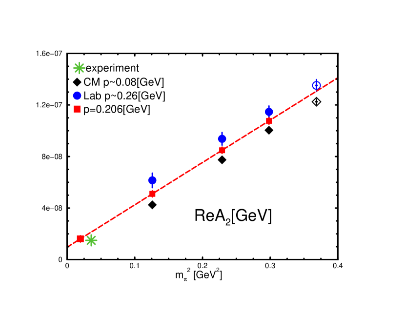
Figure 11: ${\rm Re}(A_{2})$ vs. $m_{\pi}^{2}$ in quenched QCD calculated using domain wall fermions.

Recently, the RBC collaboration has calculated the $K(P)\rightarrow\pi(P)\pi(0)$ amplitudes in the LAB frame in quenched QCD [46]. This numerical study is performed at $1/a=1.3$ GeV on the $16^{3}\times 32$ lattice with $L_{s}=12$ using domain wall fermions and the DBW2 gauge action. Using the formula of Eq. 60, the result in the LAB frame is converted into that of the infinite volume in the CM frame. A preliminary result for ${\rm Re}(A_{2})$ is shown in Fig. 11.

7 $K_{l3}$ decay

The $K_{l3}$ decays are the kaon beta decay processes: $K^{+}\rightarrow\pi^{0}l^{+}\nu_{l}$ and $K^{0}\rightarrow\pi^{-}l^{+}\nu_{l}$, where $l$ represents the electron or the muon. These decay channels play an important role in determining the CKM matrix element $|V_{us}|$. The decay rate of the $K_{l3}$ processes is given in Ref. [47]:

$$\Gamma=\frac{G_{F}^{2}}{192\pi^{3}}m_{K}^{5}\cdot|V_{us}|^{2}\cdot C^{2}\cdot|f_{+}(0)|^{2}\cdot I\cdot(1+\delta)$$ (61)

where $C$ is a Clebsch-Gordon coefficient (1 for $K^{0}$ decay; $1/\sqrt{2}$ for $K^{+}$ decay), $I$ represents the phase space integral, and $\delta$ represents radiative corrections from electroweak and electromagnetic interactions. Here, $f_{+}(0)$ is a form factor which is defined for the neutral kaon decay as

$$\langle\pi(p^{\prime})|\bar{s}\gamma_{\mu}u|K(p)\rangle=(p_{\mu}+p^{\prime}_{\mu})f_{+}(q^{2})+q_{\mu}f_{-}(q^{2})$$ (62)

where $q=p-p^{\prime}$ represents the momentum transfer. For later discussion, it is convenient to define the scalar form factor $f_{0}(q^{2})$ as

$$f_{0}(q^{2}) = f_{+}(q^{2})+\frac{q^{2}}{m_{K}^{2}-m_{\pi}^{2}}f_{-}(q^{2})$$ (63)

$$\xi(q^{2}) = \frac{f_{-}(q^{2})}{f_{+}(q^{2})}$$ (64)

The decay rate $\Gamma$ is well determined from experiment. From Ref. [48],

$$|V_{us}f_{+}(0)|=0.2173$$ (65)

Hence, if we know $f_{+}(0)$ with extremely high accuracy, we can determine $V_{us}$ with as much precision; this can impose a stringent constraint on the unitarity of the CKM matrix. The theoretical challenge on the lattice is to determine $f_{+}(0)$ with such a high precision that the uncertainty is under control within $\ll 1\%$.

Vector current conservation implies that $f_{+}(0)=1$ in the exact SU(3) limit of $m_{u}=m_{d}=m_{s}$. The Ademello-Gatto theorem implies that the deviation of $f_{+}(0)$ from unity is quadratic in the quark mass difference ($m_{s}-m_{u}$). If we expand $f_{+}(0)$ in chiral perturbation theory [49],

$$f_{+}(0)=1+f_{2}+f_{4}+{\cal O}(p^{6})$$ (66)

where $f_{i}$ represents terms of order ${\cal O}(p^{i})$. Here, $f_{2}$ does not depend on any new low energy constants which can be determined in terms of pseudoscalar meson masses and decay constants. However, $f_{4}$ does depends on new low energy constants.

The lattice technique to calculate $f_{+}(0)$ on the lattice is the double ratio method [50].

$$\frac{\langle\pi|\bar{s}\gamma_{4}u|K\rangle\langle K|\bar{u}\gamma_{4}s|\pi\rangle}{\langle\pi|\bar{u}\gamma_{4}u|\pi\rangle\langle K|\bar{s}\gamma_{4}s|K\rangle}=\frac{(m_{K}+m_{\pi})^{2}}{4m_{K}m_{\pi}}|f_{0}(q^{2}_{0})|^{2}$$ (67)

where the pion and kaon states carry zero momenta and $q_{0}^{2}=(m_{K}-m_{\pi})^{2}$. Here, note that $f_{+}(0)=f_{0}(0)$.

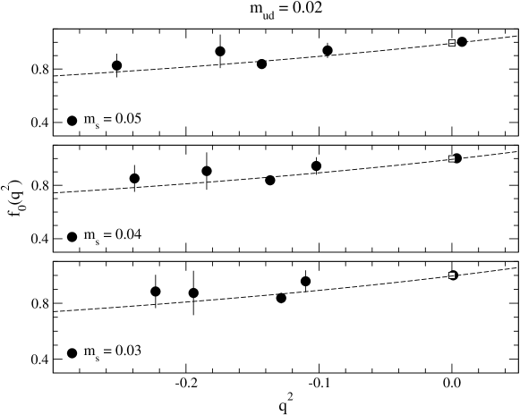
Figure 12: $f_{0}(q^{2})$ in two flavor QCD calculated by the RBC collaboration.

Eq. 67 determines $f_{0}(q_{0}^{2})$, but we need to know $f_{0}(0)=f_{+}(0)$. Hence, it is necessary to either extrapolate or interpolate in $q^{2}$ to the (Minkowski) $q^{2}=0$ point at fixed pseudoscalar meson masses. In other words, we need to insert small momenta in the kaon and pion states to change $q^{2}=(p-p^{\prime})^{2}$ (defined in Minkowski space) from $q^{2}_{0}=(m_{K}-m_{\pi})^{2}$ to negative $q^{2}$ such that we can interpolate $f_{0}(q^{2})$ to the $q^{2}=0$ point. For this purpose, we can calculate the following ratio on the lattice:

$$F(\vec{p},\vec{p}^{\prime}) = \frac{m_{K}+m_{\pi}}{E_{K}(\vec{p})+E_{\pi}(\vec{p}^{\prime})}\cdot\frac{\langle\pi(\vec{p}^{\prime})|\bar{s}\gamma_{4}u|K(\vec{p})\rangle}{\langle\pi(\vec{0})|\bar{s}\gamma_{4}u|K(\vec{0})\rangle}$$ (68)

$$= \frac{f_{+}(q^{2})}{f_{0}(q^{2}_{0})}\bigg{(}1+\frac{E_{K}(\vec{p})-E_{\pi}(\vec{p}^{\prime})}{E_{K}(\vec{p})+E_{\pi}(\vec{p}^{\prime})}\xi(q^{2})\bigg{)}$$

where $\vec{p}$ and $\vec{p}^{\prime}$ are the kaon and pion momenta respectively, $E_{K}(\vec{p})$ is the energy of kaon with a momentum $\vec{p}$, and $E_{\pi}(\vec{p}^{\prime})$ is the energy of pion with a momentum $\vec{p}^{\prime}$. Here, note that $F(\vec{0},\vec{0})=1$. In order to extract $f_{0}(q^{2})$ from Eq. 68, we first need to know $\xi(q^{2})$. It can be directly determined by measuring the following ratio:

$$R(\vec{p},\vec{p}^{\prime}) = \frac{\langle\pi(\vec{p}^{\prime})|\bar{s}\gamma_{i}u|K(\vec{p})\rangle\langle K(\vec{p}^{\prime})|\bar{s}\gamma_{4}s|K(\vec{p})\rangle}{\langle\pi(\vec{p}^{\prime})|\bar{s}\gamma_{4}u|K(\vec{p})\rangle\langle K(\vec{p}^{\prime})|\bar{s}\gamma_{i}s|K(\vec{p})\rangle}$$ (69)

$$= \frac{[(p+p^{\prime})_{i}+(p-p^{\prime})_{i}\xi(q^{2})]\cdot[E_{K}(\vec{p})+E_{K}(\vec{p}^{\prime})]}{[(E_{K}(\vec{p})+E_{\pi}(\vec{p}^{\prime}))+(E_{K}(\vec{p})-E_{\pi}(\vec{p}^{\prime}))\xi(q^{2})]\cdot[(p+p^{\prime})_{i}]}$$

After determining $\xi(q^{2})$ from this, it is then possible to determine $f_{0}(q^{2})$ by combining Eq. 67, 68 and 69.

Recently, a main goal on the lattice has been to calculate $f_{0}(0)$ in unquenched QCD. Three groups have reported results on this. First, the RBC collaboration have calculated $f_{0}(q^{2})$ in two flavor QCD using domain wall fermions at $a=0.12$ fm on the $16^{3}\times 32$ lattice [51]. In Fig. 12, we show their results for $f_{0}(q^{2})$ as a function of (Minkowski) $q^{2}$. Second, the JLQCD collaboration has calculated $f_{0}(q^{2})$ in two flavor QCD using non-perturbatively ${\cal O}(a)$ improved Wilson fermions [52]. In this calculation, the Wilson fermion action is ${\cal O}(a)$ improved but the vector current operator is not fully ${\cal O}(a)$ improved. Third, the HPQCD/FNAL collaboration has calculated $f_{0}(q^{2})$ in $2+1$ flavor QCD [53]. They use unimproved staggered fermions for the $u$ and $d$ quarks and an improved Wilson fermion for the $s$ quark. They calculate only $f_{0}(q_{0}^{2})$ using the double ratio in Eq. 67 and extrapolate to $q^{2}=0$ using the pole model by setting the free coefficient to the experimental value. These results are summarized in Table 3.

collaboration	$f_{+}(0)$
RBC	$0.968(9)(6)$ ($N_{F}=2$)
HPQCD/FNAL	$0.962(6)(9)$ ($N_{F}=2+1$)
JLQCD	$0.952(6)(-)$ ($N_{F}=2$)
Leutwyler	$0.961(8)$

Table 3: Results for $f_{+}(0)$.

8 Kaon distribution amplitude

Exclusive reactions with specific hadrons in the final and initial states have received a lot of attention. The reason is that they are dominated by rare configurations of the hadron’s constituents. One of these rare configurations is based on the hard mechanism in which only valence quark configurations contribute and all quarks have small transverse separation. The structure of the hard mechanism is relatively simple to understand. These hard contributions can be calculated in terms of hadron distribution amplitudes (DA’s) which describe the momentum fraction distribution of partons at zero transverse separation with a fixed number of constituents. In particular, the leading-twist DA’s of the pion and the nucleon have been the focus of much attention. The DA’s of the kaon are important for understanding the exclusive $B$ decays such as $B\rightarrow KK^{*}$ in the framework of QCD factorization, perturbative QCD and light cone sum rules.

The theoretical description of DA’s for the kaon is based on the relation:

$$\langle 0|\bar{u}(z)\gamma_{\nu}\gamma_{5}P(z,-z)s(-z)|K^{+}(p)\rangle_{z^{2}=0}=if_{K}p_{\nu}\int^{1}_{-1}d\xi\ \exp(i\xi p\cdot z)\ \phi_{K}(\xi,\mu^{2})$$ (70)

where $z_{\nu}$ is a light-like vector, $z^{2}=0$, $\mu$ is a renormalization scale, and $P(z,-z)$ is a path-ordered Wilson line connecting the quark and the anti-quark fields in a gauge invariant way:

$$P(z,-z)={\cal P}\exp\bigg{(}-ig\int^{z}_{-z}dy^{\mu}A_{\mu}(y)\bigg{)}$$ (71)

Here, $\phi_{K}$ is the leading twist DA of the kaon. The physical interpretation of $\xi$ is that the $s$ quark carries an $x=(1+\xi)/2$ fraction of the kaon momentum and the $\bar{u}$ anti-quark carries the rest (a $1-x=(1-\xi)/2$ fraction). The $\phi_{K}$ parametrizes the overlap of the kaon state with longitudinal momentum $p$ with the lowest Fock state consisting of a quark and an anti-quark carrying the momentum fraction $xp$ and $(1-x)p$, respectively. In Eq. 70, the convention for the normalization of $\phi_{K}$ is as follows:

$$\int^{1}_{-1}d\xi\ \phi_{K}(\xi,\mu^{2})=1$$ (72)

The conformal expansion provides a convenient tool to separate the transverse modes and the longitudinal modes. The transverse mode is formulated as a scale dependence of relevant operators and the longitudinal mode is described in terms of Gegenbauer polynomials $C^{3/2}_{n}(\xi)$:

$$\phi_{K}(\xi,\mu^{2})=\frac{3}{4}(1-\xi^{2})\bigg{(}1+\sum_{n=1}^{\infty}a_{n}(\mu^{2})C^{3/2}_{n}(\xi)\bigg{)}$$ (73)

We refer to the $a_{n}$’s as “Gegenbauer moments”.

Applying the light-cone operator product expansion (OPE) to the left-hand side of Eq. 70, we can drive the following relationship for the $n$-th moment $\langle\xi^{n}\rangle$ of the kaon DA:

$$\langle\xi^{n}\rangle(\mu^{2})=\int^{1}_{-1}d\xi\ \xi^{n}\ \phi_{K}(\xi,\mu^{2})$$ (74)

$${\cal O}^{M}_{\mu_{0},\mu_{1},\cdots,\mu_{n}}=i^{n}\bar{u}(0)\gamma_{\mu_{0}}\gamma_{5}\stackrel{{\scriptstyle\leftrightarrow}}{{D}}_{\mu_{1}}\cdots\stackrel{{\scriptstyle\leftrightarrow}}{{D}}_{\mu_{n}}s(0)$$ (75)

$$\langle 0|{\cal O}^{M}_{\{\mu_{0},\mu_{1},\ldots,\mu_{n}\}}(0)|K(p)\rangle=if_{K}\ p_{\{\mu_{0}}\ldots p_{\mu_{n}\}}\ \langle\xi^{n}\rangle$$ (76)

where the operator is defined in Minkowski space, $\stackrel{{\scriptstyle\leftrightarrow}}{{D}}=\stackrel{{\scriptstyle\rightarrow}}{{D}}-\stackrel{{\scriptstyle\leftarrow}}{{D}}$, and $\{\cdots\}$ denotes the traceless symmetrization of all the indices. The moments $\langle\xi^{n}\rangle$ are related to the Gegenbauer moments $a_{n}$ as follows:

$$a_{1} = \frac{5}{3}\langle\xi\rangle$$ (77)

$$a_{2} = \frac{7}{12}(5\langle\xi^{2}\rangle-1)$$ (78)

The theoretical mission on the lattice is to calculate the DA moments $\langle\xi^{n}\rangle$ in Euclidean space. The first step is to transcribe an operator in Euclidean space as follows:

$${\cal O}^{E}_{\mu_{0},\mu_{1},\cdots,\mu_{n}}=\bar{u}(0)\gamma_{\mu_{0}}\gamma_{5}\stackrel{{\scriptstyle\leftrightarrow}}{{D}}_{\mu_{1}}\cdots\stackrel{{\scriptstyle\leftrightarrow}}{{D}}_{\mu_{n}}s(0)$$ (79)

Since the symmetry group on the lattice is the finite group $H(4)$, which is a subgroup of $O(4)$, we need to classify ${\cal O}_{\mu_{0},\mu_{1},\cdots,\mu_{n}}$ in terms of irreducible representations of $H(4)$. The latter, in general, contains a number of irreducible representations of $O(4)$. For the first moment of the kaon, there are two types of operators:

$${\cal O}^{a}_{41} = \frac{1}{2}({\cal O}^{E}_{41}+{\cal O}^{E}_{14})$$ (80)

$${\cal O}^{b}_{44} = {\cal O}^{E}_{44}-\frac{1}{3}({\cal O}^{E}_{11}+{\cal O}^{E}_{22}+{\cal O}^{E}_{33})$$ (81)

The ${\cal O}^{a}_{41}$ operator requires a nonzero momentum component in the 1-direction. The ${\cal O}^{b}_{44}$ operator can be evaluated at zero momentum.

\psfrag{msminusmq}[t][c][1][0]{$am_{s}-am_{ud}$}\psfrag{fstmom}[c][t][1][0]{$\langle\xi\rangle^{\rm bare}$}\psfrag{Legendmass1}[c][c][1][0]{$am_{ud}=0.01$}\psfrag{Legendmass2}[c][c][1][0]{$am_{ud}=0.02$}\psfrag{Legendmass3}[c][c][1][0]{$am_{ud}=0.03$}\includegraphics[height=346.89731pt,angle={270}]{kda_1st_UKQCD.eps}

Figure 13: $\langle\xi\rangle_{K}$ in $2+1$ flavor QCD calculated by the UKQCD collaboration using domain wall fermions.

Recently, the UKQCD collaboration has calculated the first moment of the kaon DA in $2+1$ flavor QCD using domain wall fermions [54]. They use the operator of ${\cal O}^{a}_{41}$ type. In Fig. 13, we show $\langle\xi\rangle_{K}$ as a function of $m_{s}-m_{ud}$. Chiral perturbation theory predicts that there is no correction with chiral logarithms [55]. The data is certainly consistent with this prediction.

Figure 14: $\langle\xi\rangle_{K}$ in two flavor QCD calculated by the QCDSF/UKQCD collaboration using ${\cal O}(a)$ improved Wilson fermions. Top: using ${\cal O}^{a}_{41}$. Bottom: using ${\cal O}^{b}_{44}$.

The QCDSF/UKQCD collaborations have also calculated the first moment of kaon DA in two flavor QCD using ${\cal O}(a)$ improved Wilson fermions [56]. In Fig. 14, we show $\langle\xi\rangle_{K}$ as a function of $m_{K}^{2}-m_{\pi}^{2}$. In this calculation, they use operators of both ${\cal O}^{a}_{41}$ type and ${\cal O}^{b}_{44}$ type.

9 Summary and conclusion

In this paper, we have reviewed recent progress in calculating kaon spectrum, $B_{K}$, $\epsilon^{\prime}/\epsilon$, $K\rightarrow\pi\pi$ amplitudes, kaon semileptonic form factors, and moments of the kaon distribution amplitude on the lattice. Especially, there has been much progress in calculating physical observables in unquenched QCD using various lattice fermion formulations. For example, in the case of $B_{K}$, the quenched results of various groups now agree with each other within statistical and systematical uncertainty.

Through elaborate numerical studies on the pseudoscalar meson multiplet spectrum and $B_{K}$, we learned that HYP staggered fermions are remarkably better than AsqTad staggered fermions in reducing both taste symmetry breaking effects and scaling violations. However, HYP fat links are quite expensive when we calculate the fermionic force term in the rational hybrid Monte Carlo (RHMC) algorithm, because there are three SU(3) projection steps for each HYP fat link. For this reason, in Ref. [5], we proposed the $\overline{\rm Fat7}$ scheme to improve staggered fermions for the unquenched QCD simulation. The $\overline{\rm Fat7}$ scheme shares the same advantage as the HYP scheme in that the one-loop corrections for general composite operators are identical in both schemes [5]. In addition, the $\overline{\rm Fat7}$ scheme is computationally an order of magnitude cheaper for the the unquenched QCD simulation using the RHMC algorithm, mainly because we may have only one SU(3) projection step for each $\overline{\rm Fat7}$ link and the memory usage is only a quarter of that for the HYP scheme. Taking into account all these facts, we recommend using the $\overline{\rm Fat7}$ staggered fermions to generate unquenched gauge configurations using the RHMC algorithm in the future.

There are a number of fundamental difficulties for finding a good lattice version of the $Q_{6}$ and $Q_{4}$ operators in quenched QCD. A solution to this particular problem has been proposed here.

In the case of direct calculation of $K\rightarrow\pi\pi$ amplitudes, there have been a number of difficulties, in particular the Maiani Testa no-go theorem. A number of methods to get around the latter have been proposed and tested extensively. At present, the moving frame method looks quite promising and deserves further investigation. The twisted boundary condition method also looks promising but has not been discussed extensively here due to lack of space. It also deserves further attention in the future.

Most of the topics in kaon physics have their chiral behavior known from (partially) quenched chiral perturbation theory. However, the corresponding results in staggered chiral perturbation theory are not available in many cases. This also requires our attention and efforts in the future.

10 Acknowledgments

Proof-reading by David Adams is acknowledged with gratitude. Helpful discussion with S. Sharpe is also acknowledged with many thanks. W. Lee acknowledges with gratitude that the research at Seoul National University is supported by the KOSEF grant (R01-2003-000-10229-0), by the KOSEF grant of international cooperative research program, by the BK21 program, and by the DOE SciDAC-2 program.

References

- [1] Weonjong Lee and Stephen Sharpe, Partial Flavor Symmetry Restoration for Chiral Staggered Fermions, Phys. Rev. D60 (1999) 094503, [hep-lat/9905023].
- [2] C. Aubin and C. Bernard, Pion and kaon masses in staggered chiral perturbation theory, Phys. Rev. D68 (2003) 034014, [hep-lat/0304014].
- [3] K. Orginos, D. Toussaint, and R.L. Sugar, Variants of fattening and flavor symmetry restoration, Phys. Rev. D60 (1999) 054503, [hep-lat/9903032].
- [4] A. Hasenfratz and F. Knechtli, Flavor symmetry and static potential with hypercubic blocking, Phys. Rev. D64 (2001) 034504, [hep-lat/0103029].
- [5] Weonjong Lee, Perturbative improvement of staggered fermion using fat links, Phys. Rev. D66 (2002) 114504, [hep-lat/0208032].
- [6] Weonjong Lee and Stephen Sharpe, One-loop Matching coefficients for improved staggered bilinears, Phys. Rev. D66 (2002) 114501, [hep-lat/0208018].
- [7] T. Bae, et al., Pion spectrum using improved staggered fermions, PoS LAT2006 (2006) 166, [hep-lat/0610056].
- [8] C. Aubin, et al., Light pseudoscalar decay constants, quark masses, and low energy constants from three flavor lattice QCD, Phys. Rev. D70 (2004) 114501, [hep-lat/0407028].
- [9] MILC collaboration, C. Bernard et al., Update on the physics of light pseudoscalar mesons, PoS LAT2006 (2006) 163, [hep-lat/0609053].
- [10] S. Sharpe, Rooted staggered fermions: good, bad, or ugly?, PoS LAT2006 (2006) 022.
- [11] C. Aubin and C. Bernard, Pseudoscalar decay constants in staggered chiral perturbation theory, Phys. Rev. D68 (2003) 074011, [hep-lat/0306026].
- [12] S.R. Beane et al., in full QCD with domain wall valence quarks, [hep-lat/0606023].
- [13] A.J. Buras, Flavor Dynamics: CP Violation and Rare Decays, [hep-ph/0101336].
- [14] RBC and UKQCD Collaborations, Meifeng Lin et al., Light pseudoscalar decay constants from flavor domain wall fermion simulation, PoS LAT2006 (2006) 185.
- [15] JLQCD Collaboration, S. Aoki et al., Kaon b parameter from quenched lattice QCD, Phys. Rev. Lett. 80 (1998) 5271-5274, [hep-lat/9710073].
- [16] W. Lee et al., Testing improved staggered fermions with and , Phys. Rev. D71 (2005) 094501, [hep-lat/0409047].
- [17] Alpha Collaboration, P. Dimopoulos et al., A precise determination of in quenched QCD, Nucl. Phys. B749 (2006) 69-108, [hep-lat/0601002].
- [18] CP-PACS Collaboration, A. Ali Khan et al., Kaon B parameter from quenched domain wall QCD, Phys. Rev. D64 (2001) 114506, [hep-lat/0105020].
- [19] RBC Collaboration, Y. Aoki et al., The Kaon B-parameter from quenched domain-wall QCD, Phys. Rev. D64 (2001) 114506, [hep-lat/0105020].
- [20] MILC Collaboration, T. DeGrand, Kaon B parameter in quenched QCD, Phys. Rev. D69 (2004) 014504, [hep-lat/0309026].
- [21] R. Babich et al., mixing beyond the standard model and CP-violating electroweak penguins in quenched QCD with exact chiral symmetry, [hep-lat/0605016].
- [22] C. Pena, Twisted mass QCD for weak matrix elements, PoS LAT2006 (2006) 019.
- [23] HPQCD/UKQCD collaborations, E. Gamiz et al., Unquenched determination of the kaon parameter from improved staggered fermions, Phys. Rev. D73 (2006) 114502, [hep-lat/0603023].
- [24] RBC and UKQCD collaborations, S.D. Cohen and J. Noaki, on flavor Iwasaki DWF lattices, PoS LAT2006 (2006) 080.
- [25] J. Kim, et al., in unquenched QCD using improved staggered fermions, PoS LAT2006 (2006) 086, [hep-lat/0610057].
- [26] KTeV Collaboration, Measurements of Direct CP Violation, CPT Symmetry, and Other Parameters in the Neutral Kaon System, Phys. Rev. D67 (2003) 012005, [hep-ex/0208007].
- [27] NA48 Collaboration, Direct CP violation in neutral kaon decays, Pramana 62 (2004) 601-606, [hep-ex/0303037].
- [28] RBC Collaboration, Kaon matrix elements and CP violation from quenched lattice QCD: 1. The three flavor case, Phys. Rev. D68 (2003) 114506, [hep-lat/0110075].
- [29] CP-PACS Collaboration, Calculation of non-leptonic kaon decay amplitudes from matrix elements in quenched domain-wall QCD, Phys. Rev. D68 (2003) 114501, [hep-lat/0108013].
- [30] M. Golterman and E. Pallante, Effects of Quenching and Partial Quenching on Penguin Matrix Elements, JHEP 0110 (2001) 037, [hep-lat/0108010].
- [31] T. Bhattacharya et al., Calculating using HYP staggered fermion, Nucl. Phys. B (Proc. Suppl.) 140 (2005) 369-371, [hep-lat/0409046].
- [32] T. Bhattacharya et al., Weak Matrix Elements for CP violation, Nucl. Phys. B (Proc. Suppl.) 106 (2002) 311-313, [hep-lat/0111004].
- [33] RBC Collaboration, C. Aubin et al., Systematic effects of the quenched approximation on the strong penguin contribution to , Phys. Rev. D74 (2006) 034510, [hep-lat/0603025].
- [34] M. Golterman and E. Pallante, Quenched penguins and the rule, Phys. Rev. D74 (2006) 014509, [hep-lat/0602025].
- [35] M. Golterman and S. Peris, Analytic estimates for penguin operators in quenched QCD, Phys. Rev. D68 (2003) 094506, [hep-lat/0306028].
- [36] K. Choi and W. Lee, , and RG evolution for , Nucl. Phys. B (Proc. Suppl.) 140 (2005) 384-386, [hep-lat/0409020].
- [37] L. Maiani and M. Testa, Final state interactions from Euclidean correlation functions., Phys. Lett. B245 (1990) 585.
- [38] M. Luscher and U. Wolff, How To Calculate The Elastic Scattering Matrix In Two-Dimensional Quantum Field Theories By Numerical Simulation, Nucl. Phys. B339 (1990) 222.
- [39] H.R. Fiebig et al., On the channel interaction in the chiral limit, Nucl. Phys. B (Proc. Suppl.) 73 (1999) 252.
- [40] CP-PACS Collaboration, S. Aoki et al., pion scattering phase shift with Wilson fermions, Phys. Rev. D 67 (2003) 014502, [hep-lat/0209124].
- [41] Changhoan Kim, with physical final state, Nucl. Phys. B (Proc. Suppl.) 140 (2005) 381-383.
- [42] K. Rummukainen and S. Gottlieb, RESONANCE SCATTERING PHASE SHIFTS ON A NON–REST FRAME LATTICE, Nucl. Phys. B450 (1995) 397, [hep-lat/9503028].
- [43] N. Christ et al., Finite Volume Corrections to the Two-Particle Decay of States with Non-Zero Momentum, Phys. Rev. D 72 (2005) 114506, [hep-lat/0507009].
- [44] C. Kim et al., Finite-Volume Effects for Two-Hadron States in Moving Frames, Nucl. Phys. B727 (2005) 218-243, [hep-lat/0507006].
- [45] L. Lellouch and M. Luscher, Weak transition matrix elements from finite-volume correlation functions, Comm. Math. Phys. 219 (2001) 31-44, [hep-lat/0003023].
- [46] RBC Collaboration, T. Yamazaki et al., calculation with interaction effect on finite volume, PoS LAT2006 (2006) 100.
- [47] H. Leutwyler and M. Roos, Determination of the elements and of the Kobayashi-Maskawa matrix, Z. Phys. C 25 (1984) 91.
- [48] E. Blucher et al., Status of the Cabibbo Angle, Proceedings of the CKM 2005 Workshop, [hep-ph/0512039].
- [49] J. Bijnens and P. Talavera, decays in chiral perturbation theory, Nucl. Phys. B669 (2003) 341-362, [hep-ph/0303013].
- [50] D. Becirevic et al., The vector form factor at zero momentum transfer on the lattice, Nucl. Phys. B705 (2005) 339-362, [hep-ph/0403217].
- [51] C. Dawson et al., Vector form factor in semileptonic decay with two flavors of dynamical domain-wall quarks, [hep-ph/0607162].
- [52] JLQCD Collaboration, N. Tsutsui et al., Kaon semileptonic decay form factors in two-flavor QCD, PoS LAT2005 (2005) 357, [hep-lat/0510068].
- [53] M. Okamoto, B, D, K decays and CKM matrix from lattice QCD, FPCP04 proceeding, [hep-lat/0412044].
- [54] UKQCD Collaboration, P.A. Boyle et al., Lattice computation of the first moment of the Kaon’s distribution amplitude, [hep-lat/0607018].
- [55] J.W. Chen and I.W. Stewart, Model Independent Results for SU(3) Violation in Light-Cone Distribution Functions, Phys. Rev. Lett. 92 (2004) 202001, [hep-ph/0311285].
- [56] QCDSF/UKQCD Collaboration, V.M. Braun et al., Moments of pseudoscalar meson distribution amplitudes from the lattice, [hep-lat/0606012].