Pion spectrum using improved staggered fermions

Abstract:

We present results for the pion multiplet spectrum calculated using both unimproved staggered fermions and improved HYP-smeared staggered fermions. In the case of unimproved staggered fermions, we observe (consistent with previous work) that ${\cal O}(a^{2})$ taste symmetry breaking effects are large and comparable to the $\approx{\cal O}(p^{2})$ contributions to their masses. Higher order ${\cal O}(a^{2}p^{2})$ effects are also substantial enough to be seen. For HYP-smeared staggered fermions, we find that taste breaking is much reduced. The ${\cal O}(a^{2})$ effects are observable, but are noticeably smaller than those obtained with AsqTad-improved staggered fermions, and much smaller than those obtained using unimproved staggered fermions, while ${\cal O}(a^{2}p^{2})$ effects are suppressed to such a level that we cannot observe them given our statistical errors. From this numerical study, we conclude that HYP staggered fermions are significantly better that AsqTad fermions from the perspective of taste symmetry breaking.

1 Pion spectrum with staggered fermions

Staggered fermions have four tastes, leading to 16 tastes of flavor non-singlet pions. These have the spin-taste structure $(\gamma_{5}\otimes\xi_{F})$ with $\xi_{F}\in\{I,\xi_{5},\xi_{\mu},\xi_{\mu 5},\xi_{\mu\nu}=\frac{1}{2}[\xi_{\mu},\xi_{\nu}]\}$. These states fall into 8 irreducible representations of the lattice timeslice group [1]: $\{I\}$, $\{\xi_{5}\}$, $\{\xi_{i}\}$, $\{\xi_{4}\}$, $\{\xi_{i5}\}$, $\{\xi_{45}\}$, $\{\xi_{ij}\}$, and $\{\xi_{i4}\}$. The pion with taste $\xi_{5}$ is the Goldstone pion corresponding to the axial symmetry which is exact when $m=0$ and is broken spontaneously. The properties of the pion spectrum can be studied using staggered chiral perturbation theory [2, 3]. It is shown in Ref. [2] that, at leading order in a joint expansion in $p^{2}$ and $a^{2}$, the pion spectrum respects an SO(4) subgroup of the full SU(4) taste symmetry. In other words, the taste symmetry breaking happens in two steps: at ${\cal O}(p^{2})\approx{\cal O}(a^{2})$ the SU(4) taste symmetry is broken down to the SO(4) taste symmetry, while at ${\cal O}(a^{2}p^{2})$ the SO(4) taste symmetry is broken down to the discrete spin-taste symmetry $SW_{4}$ [2]. As a consequence of this analysis, we expect that, to good approximation the pions will lie in 5 irreducible representations of SO(4) taste symmetry: $\{I\}$, $\{\xi_{5}\}$, $\{\xi_{\mu}\}$, $\{\xi_{\mu 5}\}$, $\{\xi_{\mu\nu}\}$.

The splittings between the pion multiplets are a non-perturbative measure of taste-symmetry breaking, and can be used to measure the efficacy of different improvement schemes. The more effective the improvement, the smaller the expected splitting. In this paper, we present results for the pion spectrum calculated using different choices of staggered fermions—unimproved, HYP and AsqTad—and compare their splitting patterns in order to determine which improvement scheme is better or more efficient in reducing the taste symmetry breaking.

In a recent study of $B_{K}$ using staggered chiral perturbation theory [4], it was found that loop contributions from non-Goldstone pions (with $\xi_{F}\neq\xi_{5}$) was much larger than that from the Goldstone pion. One motivation for the present study is to determine all the pion masses so that they can be used as inputs into the chiral perturbation theory fit for $B_{K}$.

2 Cubic symmetry of the source

In order to select a specific pion taste and to exclude all others, it is necessary to choose sources and/or sinks to lie in specific representations of the timeslice group. Here we discuss how this is done for the sources. We consider only sources with vanishing physical three-momentum. We adopt two different methods, one the “cubic U(1) source” and the other the “cubic wall-source”. We first fix gauge configurations to Coulomb gauge. Then propagators are obtained, as usual, by solving the following Dirac equation with $h$ set to a specific source type.

$$(D+m)\chi(x)=h(y)$$ (1)

$$\chi(x,a)=\sum_{y,b}G(x,a;y,b)h(y,b)$$ (2)

where $a,b$ are color indices and $G(x;y)$ is a quark propagator. For the cubic U(1) source at time slice $t$ we choose $h(y)$ as follows:

$$h(y,b)=\delta_{y_{4},t}\delta^{3}_{\vec{y},2\vec{n}+\vec{A}}\xi(\vec{n},b)\ ,\mbox{ and }\xi(\vec{n},b)\in U(1)$$ (3)

$$\lim_{N\rightarrow\infty}\frac{1}{N}\sum_{\xi}\xi(\vec{n},c)\xi^{*}(\vec{n}^{\prime},c^{\prime})=\delta_{\vec{n},\vec{n}^{\prime}}\delta_{c,c^{\prime}}$$ (4)

where $\vec{A}$ is a cubic vector $\in\{(0,0,0),(1,0,0),\cdots,(1,1,1)\}$, $N$ is the number of random vectors and $\vec{n}\in Z^{3}$. Similarly, in order to set up the cubic wall source at time slice $t$, we define $h(y,b)$ as follows:

$$h(y,b)=\delta_{y_{4},t}\delta^{3}_{\vec{y},2\vec{n}+\vec{A}}\xi(b)\ ,\mbox{ and }\xi(b)\in U(1)$$ (5)

$$\lim_{N\rightarrow\infty}\frac{1}{N}\sum_{\xi}\xi(c)\xi^{*}(c^{\prime})=\delta_{c,c^{\prime}}$$ (6)

In other words, the random vectors are the same on all spatial hypercubes. Note that there are eight sources of each type, depending on the choice of $\vec{A}$. By combining these we can project onto particular representations of the timeslice group. We do not know, however, which type of source is more efficient; this can only be determined through a numerical study.

parameter	value
$\beta$	6.0 (quenched QCD, Wilson plaquette action)
$1/a$	1.95 GeV
geometry	$16^{3}\times 64$
# of confs	218
gauge fixing	Coulomb
bare quark mass	0.005, 0.01, 0.015, 0.02, 0.025, 0.03
$Z_{m}$	$\approx 2.5$

Table 1: Simulation parameters for unimproved staggered fermions

3 Operator Transcription

We use two different methods to construct bilinear operators: the “Kluberg-Stern method” [5] and the “Golterman method” [1]. In the Kluberg-Stern method, a bilinear operator is expressed as

$$O_{S,F}=\sum_{A,B}\bar{\chi}(A)\overline{(\gamma_{S}\otimes\xi_{F})}_{A,B}\chi(B)$$ (7)

$$\overline{(\gamma_{S}\otimes\xi_{F})}_{A,B}=\frac{1}{4}{\rm Tr}(\gamma_{A}^{\dagger}\gamma_{S}\gamma_{B}\gamma_{F}^{\dagger})$$ (8)

where $A,B$ is a hypercubic vector $\in\{(0,0,0,0),(1,0,0,0),\cdots,(1,1,1,1)\}$, $\gamma_{S}$ ($\xi_{F}$) represents the spin (taste). The operator is made gauge invariant by fixing each timeslice to Coulomb gauge, so that spatial links are not required, and inserting appropriate time-directed links if $S_{4}\neq F_{4}$. In the Golterman method, the bilinears are

$$O_{S,F}=\eta_{S,F}(x)\bar{\chi}(x)M_{S,F}\chi(x)$$ (9)

$$M_{S,F}\chi(x)=\prod_{\mu=1,2,3}\Big{[}(1-|S_{\mu}-F_{\mu}|)+|S_{\mu}-F_{\mu}|D_{\mu}\Big{]}\chi(x)$$ (10)

$$D_{\mu}\chi(x)=\frac{1}{2}\Big{[}\chi(x+\hat{\mu})+\chi(x-\hat{\mu})\Big{]}$$ (11)

where $\eta_{S,F}(x)$ is a phase factor given in Ref. [1], and gauge invariance is maintained as for the Kluberg-Stern operators.

The Kluberg-Stern method gives bilinears that are only approximate representations of the timeslice group whereas the Golterman method sorts out the bilinears according to true irreducible representations [1]. We apply both methods to our numerical study and the results will be compared in the next section.

4 Numerical Study with unimproved staggered fermions

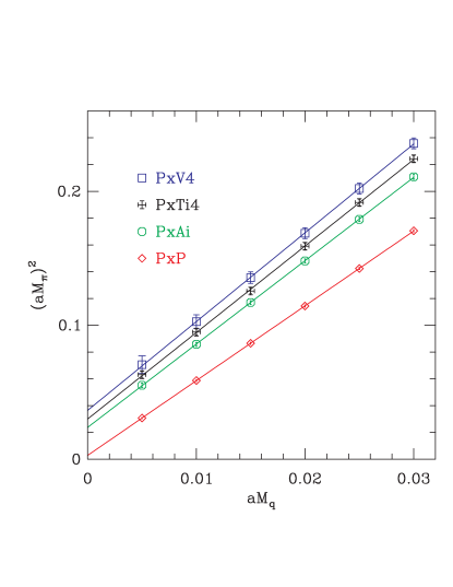
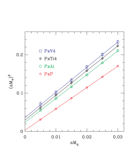
Figure 1: $(am_{\pi})^{2}$ vs. $am_{q}$ for unimproved staggered fermions: (left) using the Kluberg-Stern method; (right) using the Golterman method; In both calculations, the sources are set to cubic U(1) source.

The parameters for the numerical study using unimproved staggered fermions are summarized in Table 1. In Fig. 1 we show $(am_{\pi})^{2}$ as a function of quark masses using bilinear operators with spin-taste $\gamma_{5}\otimes\xi_{4}$, $\gamma_{5}\otimes\xi_{i4}$, $\gamma_{5}\otimes\xi_{i5}$, and $\gamma_{5}\otimes\xi_{5}$. We find essentially no difference between the Kluberg-Stern method (left panel) and the Golterman method (right panel). The Kluberg-Stern operator includes the Golterman operator as the leading term, as well as operators with derivatives having different spin-tastes. The latter couple to different states which should be projected against by the sources. Nevertheless, one might expect the Kluberg-Stern operators to have a more noisy signal. In fact, we see that the signals with the two methods are essentially identical.

In Fig. 1, we also observe that the splitting between the pion multiplets are comparable to the light pion masses, implying that ${\cal O}(a^{2})\approx{\cal O}(p^{2})$. In addition, we observe that the slopes are different for various tastes, implying that ${\cal O}(a^{2}p^{2})$ terms are significant.

5 Numerical Study with HYP staggered fermions

Using the same set of gauge configurations as in Sec. 4, we study the pion spectrum with HYP-smeared staggered fermions [6]. The parameters for the HYP fat links are set to the HYP (II) condition in Ref. [7]. In the numerical study, we use quark masses of 0.01, 0.02, 0.03, 0.04, 0.05. Note that $Z_{m}\approx 1$ for HYP staggered fermions whereas $Z_{m}\approx 2.5$ for unimproved staggered fermions. Hence, the physical quark masses in this study are comparable to those for the unimproved staggered fermions considered above.

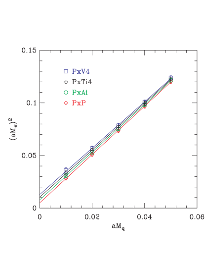
Figure 2: $(am_{\pi})^{2}$ vs. $am_{q}$ for HYP staggered fermions: (left) using the cubic U(1) source; (right) using the cubic wall source; In both calculations, the operators are constructed using the Golterman method.

In Fig. 2, we show $(am_{\pi})^{2}$ as a function of quark mass and compare the results of the cubic U(1) source (left) with those of the cubic wall source (right). This comparison indicates there is essentially no difference between the two sources in practice. In Fig. 2, we observe that the splittings between the pions are significantly suppressed, down to the $2\sigma$ level in our data set, implying that ${\cal O}(a^{2})\ll{\cal O}(p^{2})$. In addition, the slopes for different tastes are equal within statistical uncertainty, showing that improvement reduces the ${\cal O}(a^{2}p^{2})$ effects as well.

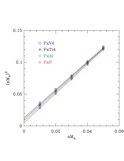
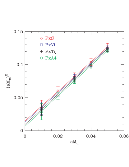
Figure 3: $(am_{\pi})^{2}$ vs. $am_{q}$: (left) for the operators local in time; (right) for the operators non-local in time; In both cases, we use the Kluberg-Stern method to construct the operators and we also choose cubic U(1) sources.

We can divide the pion bilinear operators into two categories: one is local in time ($\gamma_{5}\otimes\xi_{5}$, $\gamma_{5}\otimes\xi_{4}$, $\gamma_{5}\otimes\xi_{i5}$, and $\gamma_{5}\otimes\xi_{i4}$) and the other is non-local in time ($\gamma_{5}\otimes 1$, $\gamma_{5}\otimes\xi_{i}$, $\gamma_{5}\otimes\xi_{45}$, and $\gamma_{5}\otimes\xi_{ij}$). In the case of sink operators local in time, we can construct the source operators with the same spin and taste structure. However, in the case of sink operators non-local in time, we cannot impose the same spin and taste on the source operators, because the source is local in time by construction. Since we want to select a pion with a specific taste, we do not have any other choice for the taste but we do have the freedom to choose the spin: we may choose either pseudoscalar ($\gamma_{5}$) or axial vector ($\gamma_{45}$). Hence, in the case of sink operators non-local in time, we choose axial current as a source operator, which is local in time. For example, if the sink operator is $\gamma_{5}\otimes\xi_{i}$ (non-local in time), we choose $\gamma_{45}\otimes\xi_{i}$ (local in time) as the source operator. In Fig. 3, we show $(am_{\pi})^{2}$ as a function of quark mass for operators local in time (left) and for operators non-local in time (right). We see that the signals for the operators non-local in time are noisier than those for the local operators.

We also observe that the pattern of pion multiplet spectrum is in the following order, which is the same for unimproved staggered fermions and AsqTad staggered fermions:

$$m_{\pi}(\xi_{5})<m_{\pi}(\xi_{\mu 5})<m_{\pi}(\xi_{\mu\nu})<m_{\pi}(\xi_{\mu})<m_{\pi}(I)$$ (12)

6 Comparison of AsqTad and HYP staggered fermions

In Fig. 4, we compare the results of AsqTad staggered fermions (left) with those of HYP staggered fermions (right). The AsqTad staggered fermion data comes originally from Ref. [8]. It has $a=0.125$ fm (MILC coarse lattice) whereas the results for HYP-smeared staggered fermions are on a finer lattice with $a\approx 0.1$ fm. Nevertheless, since the gauge part of the AsqTad action is Symanzik improved, while our calculation uses the unimproved Wilson gauge action, we expect that the scaling violations from the background gauge configurations to be similar. The physical quark masses are also similar.

In the case of AsqTad staggered fermions, we observe that the taste-symmetry breaking is of the same order as the light pion masses. In other words, ${\cal O}(a^{2})\approx{\cal O}(p^{2})$ for the AsqTad action. In addition, we notice that the slopes for different tastes are very close, implying that this manifestation of ${\cal O}(a^{2}p^{2})$ terms is very small. By contrast, with HYP-smeared staggered fermions we see that both ${\cal O}(a^{2})$ and ${\cal O}(a^{2}p^{2})$ effects are very small. We conclude that HYP staggered fermions are significantly better than AsqTad staggered fermions from the standpoint of taste symmetry breaking.

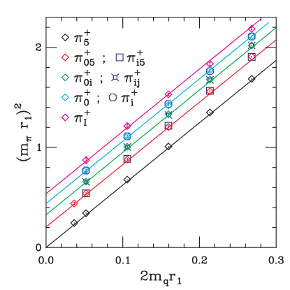
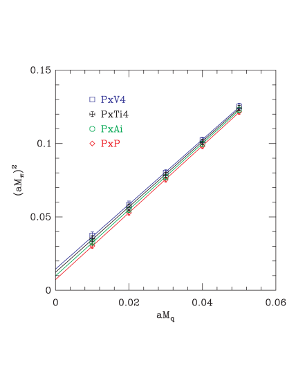
Figure 4: $(am_{\pi})^{2}$ vs. $am_{q}$: (left) for AsqTad staggered fermions; (right) for HYP staggered fermions (the Kluberg-Stern method, cubic wall source)

7 Acknowledgment

W. Lee acknowledges with gratitude that the research at Seoul National University is supported by the KOSEF grant (R01-2003-000-10229-0), by the KOSEF grant of international cooperative research program, by the BK21 program, and by the US DOE SciDAC-2 program. The work of S. Sharpe is supported in part by the US DOE grant no. DE-FG02-96ER40956, and by the US DOE SciDAC-2 program.

References

- [1] Maarten Golterman, Staggered Mesons, Nucl. Phys. B273 (1986) 663-676.
- [2] Weonjong Lee and Stephen Sharpe, Partial Flavor Symmetry Restoration for Chiral Staggered Fermions, Phys. Rev. D60 (1999) 094503, [hep-lat/9905023].
- [3] C. Aubin and C. Bernard, Pion and kaon masses in staggered chiral perturbation theory, Phys. Rev. D68 (2003) 034014, [hep-lat/0304014].
- [4] Ruth S. Van de Water, Stephen R. Sharpe, in staggered chiral perturbation theory, Phys. Rev. D73 (2006) 014003, [hep-lat/0507012].
- [5] H. Kluberg-Stern, et al., Flavors of Lagrangian Suskind fermions, Nucl. Phys. B220 (1983) 447; D. Verstegen, Symmetry properties of fermionic bilinears , Nucl. Phys. B249 (1985) 685.
- [6] A. Hasenfratz and F. Knechtli,, Flavor symmetry and the static potential with hypercubic blocking, Phys. Rev. D64 (2002) 034504, [hep-lat/0103029].
- [7] Weonjong Lee and Stephen Sharpe, Perturbative matching of staggered four-fermion operators with hypercubic fat links, Phys. Rev. D68 (2003) 054510, [hep-lat/0306016].
- [8] C. Aubin, et al., Light pseudoscalar decay constants, quark masses, and low energy constants from three flavor lattice QCD, Phys. Rev. D70 (2004) 114501, [hep-lat/0407028].