The QCD equation of state with asqtad staggered fermions

Abstract:

We report on our result for the equation of state (EOS) with a Symanzik improved gauge action and the asqtad improved staggered fermion action at $N_{t}=4$ and 6. In our dynamical simulations with 2+1 flavors we use the inexact R algorithm and here we estimate the finite step-size systematic error on the EOS. Finally we discuss the non-zero chemical potential extension of the EOS and give some preliminary results.

1 Introduction

The determination of the equation of state (EOS) of strongly interacting matter on the lattice requires actions with small discretization effects, a realistic light quark spectrum and good control over the systematic errors in order for the result to be relevant in helping to understand experimental findings. For our thermodynamics studies we use the asqtad quark action [1] for 2+1 flavors, combined with a one-loop Symanzik improved gauge action [2]. Both actions are highly improved and have discretization errors of $O(\alpha_{s}a^{2},\,a^{4})$ and $O(\alpha_{s}^{2}a^{2},\,a^{4})$, respectively. We do our simulations along trajectories of constant physics using the dynamical R algorithm [3] and thus our calculations are subject to finite step-size errors. Here we describe the method we use to estimate and correct for this systematic error.

To approximate the experimental conditions as closely as possible we have started a project which extends our EOS calculation to a small non-zero chemical potential. For this purpose we use the Bielefeld–Swansea Taylor expansion method [4] and preliminary results for the EOS at a set of chemical potentials are presented.

2 Simulation overview

We study the quark-gluon system at a range of temperatures along trajectories of constant physics. Such trajectories are defined by keeping the ratios $m_{\pi}/m_{\rho}$ and $m_{\eta_{ss}}/m_{\phi}$ fixed while changing $a$ at a constant $N_{t}$. We work with two approximate trajectories; for both of them the heavy (strange) quark mass $m_{s}$ is fixed to the physical value within about 20%. The light quark masses for the two trajectories are $m_{ud}\approx 0.2m_{s}$ ($m_{\pi}/m_{\rho}\approx 0.4$) and $m_{ud}\approx 0.1m_{s}$ ($m_{\pi}/m_{\rho}\approx 0.3$), respectively. For both trajectories we have performed calculations at $N_{t}=6$. In addition, a study at $N_{t}=4$ was done for the $m_{ud}\approx 0.1m_{s}$ trajectory in order to compare the effect of the larger discretization errors on the EOS. The constant physics trajectories are parameterized with RG-inspired formulae using the hadron spectrum data at certain anchor points (see [5] for explicit formulae).

The lattice gauge configurations are generated with step sizes in the R algorithm chosen to be the smaller of 0.02 and $2m_{ud}/3$, and occasionally smaller still. Most of the gauge configurations used for the analysis were generated before the RHMC algorithm [6] became known. Since Lattice 2005 [5], we have doubled the statistics and added a new high-temperature run at $\beta=7.08$ ($a\approx 0.086$ fm) and a zero-temperature run at $\beta=6.275$ ($a\approx 0.232$ fm) for the $N_{t}=4$ case. For both trajectories new zero- and high-temperature runs at $\beta=6.85$ ($a\approx 0.110$ fm) were included as well. For the list of the rest of the run parameters see [5]. The lattice spacing $a$ has been determined at zero temperature using the heavy quark potential (”$r_{1}$”) with the overall scale set by the $\Upsilon$ 1S-2S mass splitting [7]. We fit all the available data to an appropriate one-loop RG-inspired formula [5] which gives the lattice spacing as a function of the quark masses and the gauge coupling and allows us to determine the temperature along the constant physics trajectories.

3 The EOS analytic form

We determine the EOS using the integral method [8], where the pressure is calculated as an integral of the interaction measure and the energy density is a linear combination of both:

$$Ia^{4} = -6\frac{d\beta_{\rm pl}}{d\ln a}\Delta\left\langle P\right\rangle-12\frac{d\beta_{\rm rt}}{d\ln a}\Delta\left\langle R\right\rangle-16\frac{d\beta_{\rm ch}}{d\ln a}\Delta\left\langle C\right\rangle$$ (1)

$$-\sum_{f}\frac{n_{f}}{4}\left[\frac{d(m_{f}a)}{d\ln a}\Delta\left\langle\bar{\psi}\psi\right\rangle_{f}+\frac{du_{0}}{d\ln a}\Delta\left\langle\bar{\psi}\,\frac{dM}{du_{0}}\,\psi\right\rangle_{f}\right],$$

$$pa^{4} = -\int_{\ln a_{0}}^{\ln a}I(a^{\prime})(a^{\prime})^{4}d\ln a^{\prime},$$ (2)

$$\varepsilon a^{4} = Ia^{4}+3pa^{4}.$$ (3)

For physics quantities and parameter definitions in the above see [5].

4 Systematic errors and EOS results

Our calculation is affected by the following systematic errors: finite volume effects, choice of the lower integration limit in Eq. (2) and the finite step-size error in the R algorithm. The first two errors are relatively straightforward to estimate. By conducting an EOS calculation along the $m_{ud}\approx 0.1m_{s}$, $N_{t}=4$ trajectory on a small ($8^{3}\times 4$) volume and comparing it with the result of the calculation on a larger ($12^{3}\times 4$) volume, we have determined that the finite volume effects are negligible. To estimate the error introduced by postulating the lower integration limit in Eq. (2) to be at the coarsest available lattice scale in our simulations on a given trajectory, we have calculated the pressure of an ideal pion gas at the corresponding lowest available temperature points. The value of the ideal pion gas pressure at these temperatures is about as large as the statistical errors we have. Thus, we have ignored this systematic error as well.

The finite step-size error determination is a much more involved procedure. We have performed some additional simulations at different step sizes using the R algorithm and, recently, some using the exact RHMC algorithm. We measured most of the gluonic and the fermionic observables in Eq. (1) at different step sizes. Figure 1 shows the step-size dependence of the plaquette and the light chiral condensate for one case.

Figure 1: Plaquette (left panel) and chiral condensate (right panel) vs the squared step size $\epsilon^{2}$ for the improved action for the ensemble at $\beta=6.467$, $am_{ud}=0.01676$ and $am_{s}=0.0821$. The squared step size used for production of this ensemble is 0.0001.

The step-size error in the plaquette variable has a potentially significant effect on the EOS, whereas the step-size error in the chiral condensate (and the rest of the fermionic observables) is negligible. We have found that the gluonic observables (plaquette, rectangle and parallelogram) have similar step-size dependence slopes. For this reason we have concentrated on studying the finite step-size corrections mainly for the plaquettes and applied the same corrections to the rest of the gluonic observables. Figure 2 shows the plaquette slopes determined from a set of runs with different step sizes for both trajectories.

Figure 2: Plaquette slopes for the $m_{ud}\approx 0.1m_{s}$ trajectory (left) and the $m_{ud}\approx 0.2m_{s}$ trajectory (right) vs. the chiral condensate.

We see that for the $m_{ud}\approx 0.2m_{s}$ trajectory the slopes are small which means that the finite step-size errors can be ignored in this case. For the $m_{ud}\approx 0.1m_{s}$ trajectory we have more data for the plaquette slopes from both $N_{t}=6$ and 4 simulations. We fit our data to a quadratic form and use it to correct the EOS. Still, even in this case the finite step-size errors are quite small. The finite step-size corrections which we showed at the Lattice 2006 conference were overestimated due to the limited amount of data on step-size dependence we had at that time. Figure 3 and 4 show our results for the interaction measure, pressure and energy density after the small finite step-size corrections in the $m_{ud}\approx 0.1m_{s}$ trajectory have been included.

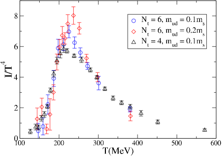
Figure 3: Interaction measure vs. temperature for both constant physics trajectories and $N_{t}$’s.

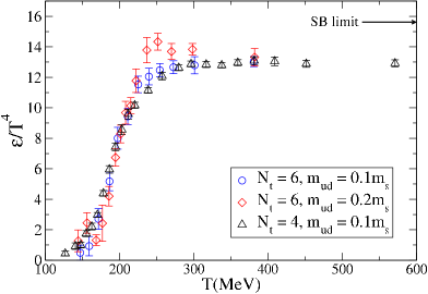
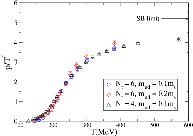
Figure 4: Energy density (left) and pressure (right) vs. temperature for both constant physics trajectories and $N_{t}$’s.

5 The EOS with non-zero chemical potential

To include a non-zero chemical potential in the EOS calculation we use the Bielefeld–Swansea Taylor expansion method [4]. According to this method the pressure can be expanded as:

$$\frac{p}{T^{4}}=\frac{\ln Z}{VT^{3}}=\sum_{n,m=0}^{\infty}c_{nm}(T)\left(\frac{\bar{\mu}_{l}}{T}\right)^{n}\left(\frac{\bar{\mu}_{h}}{T}\right)^{m},$$ (4)

where $Z$ is the partition function, and $\bar{\mu}_{l,h}$ are the chemical potentials for the light and heavy quarks, respectively. We note that the problems of rooted staggered fermions at non-zero chemical potential [9] are not relevant here since all the expansion coefficients are evaluated in the $\mu_{l,h}=0$ theory. Due to CP symmetry the non-zero terms in the series have even $n+m$. The non-zero coefficients in the above are

$$c_{nm}(T)=\frac{1}{n!}\frac{1}{m!}\frac{N_{t}^{3}}{N_{s}^{3}}\frac{\partial^{n+m}\ln Z}{\partial(\mu_{l}N_{t})^{n}\partial(\mu_{h}N_{t})^{m}}\biggr{|}_{\mu_{l,h}=0}\quad,$$ (5)

where now the $\mu_{l,h}$ are the chemical potentials in lattice units. Similarly, for the interaction measure we have:

$${I\over T^{4}}=-{N_{t}^{3}\over N_{s}^{3}}{d\ln Z\over d\ln a}=\sum_{n,m}^{\infty}b_{nm}(T)\left({\bar{\mu}_{l}\over T}\right)^{n}\left({\bar{\mu}_{h}\over T}\right)^{m},$$ (6)

where again only terms with even $n+m$ are non-zero and

$$b_{nm}(T)=\left.-{1\over n!m!}{N_{t}^{3}\over N_{s}^{3}}{\partial^{n+m}\over\partial(\mu_{l}N_{t})^{n}\partial(\mu_{h}N_{t})^{m}}\right|_{\mu_{l,h}=0}\left({d\ln Z\over d\ln a}\right).$$ (7)

To determine the EOS, we need to calculate derivatives of the asqtad fermion matrix such as

$$\frac{\partial^{n}\ln\det M_{l,h}}{\partial\mu_{l,h}^{n}},\hskip 28.45274pt\frac{\partial^{n}\,\mbox{Tr}M_{l,h}^{-1}}{\partial\mu_{l,h}^{n}},\hskip 28.45274pt\frac{\partial^{n}\,\mbox{Tr}(M_{l,h}^{-1}\frac{dM_{l,h}}{du_{0}})}{\partial\mu_{l,h}^{n}}.$$ (8)

These derivatives are estimated on the ensembles of lattices along a constant physics trajectory using 200 random sources in the region of the phase transition/crossover and 100 sources outside that region. We intend to study the EOS up to $O(\mu^{6})$ on both constant physics trajectories. Currently we have data for only one of them and not enough statistics to resolve the sixth-order terms. Thus the preliminary results for the EOS we present here are calculated to $O(\mu^{4})$ on the $m_{ud}\approx 0.1m_{s}$, $N_{t}=4$ trajectory only. We also set $\mu_{h}=0$ here. Figure 5 shows our result for some of the coefficients involved in Eq. (4). An interesting feature is that the coefficients quickly reach the continuum Stefan-Boltzmann limit above $T_{c}$.

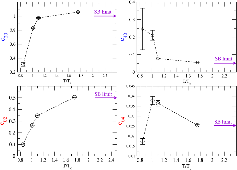
Figure 5: Some Taylor coefficients in the pressure expansion for the $m_{ud}\approx 0.1m_{s}$, $N_{t}=4$ trajectory.

The pressure and energy density corrections due to the non-zero chemical potential are shown in Figure 6.

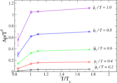
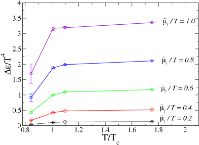
Figure 6: Pressure correction $\Delta p=p(\mu_{l})-p(\mu_{l}=0)$ and energy density correction $\Delta\varepsilon=\varepsilon(\mu_{l})-\varepsilon(\mu_{l}=0)$ for the $m_{ud}\approx 0.1m_{s}$, $N_{t}=4$ trajectory to $O(\mu^{4})$ and at $\mu_{h}=0$.

6 Conclusions

We have calculated the EOS along two constant physics trajectories with $m_{ud}\approx 0.1m_{s}$ and $0.2m_{s}$ using the R algorithm. To estimate the finite step-size errors we have performed a number of additional R algorithm simulations at different step-sizes and a few RHMC simulations along the constant physics trajectories. The analysis of this additional data shows that the finite step-size errors are negligible on the $m_{ud}\approx 0.2m_{s}$ trajectory and small (in most cases less a than few percent) on the $m_{ud}\approx 0.1m_{s}$ trajectory.

We have started a non-zero chemical potential study of the EOS with 2+1 flavors using the Bielefeld–Swansea Taylor expansion method and presented preliminary EOS results for a number of different $\bar{\mu}_{l}/T$ values.

Acknowledgments

We thank Maarten Golterman for discussions. This work was supported by the US DOE and NSF. Computations were performed at CHPC (Utah), FNAL, FSU, IU, NCSA and UCSB.

References

- [1] K. Orginos and D. Toussaint, Phys. Rev. D 59, 014501 (1999); Nucl. Phys. Proc. Suppl. 73, 909 (1999); G. P. Lepage, Nucl. Phys. Proc. Suppl. 60 A, 267 (1998); Phys. Rev. D 59, 074502 (1999).
- [2] K. Symanzik, Plenum, New York 1980, 313.
- [3] S. Gottlieb et al., Phys. Rev. D 35, 2531 (1987).
- [4] C.R. Allton et al., Phys. Rev. D 66, 074507 (2002) [hep-lat/0204010].
- [5] C. Bernard et al., Proc. Sci. LAT2005, 156 (2005) [hep-lat/0509053].
- [6] M.A. Clark et al., Nucl. Phys. Proc. Suppl. 140, 835 (2005) [hep-lat/0409133].
- [7] M. Wingate et al., Phys. Rev. Lett. 92, 162001 (2004); A. Gray et al., Phys. Rev. D 72, 094507 (2005) [hep-lat/0507013].
- [8] J. Engels et al., Phys. Lett. B 252, 625 (1990).
- [9] M. Golterman, Y. Shamir and B. Svetitsky, [hep-lat/0602026].