Electromagnetic and spin polarisabilities in lattice QCD

Abstract:

We discuss the extraction of the electromagnetic and spin polarisabilities of nucleons from lattice QCD [1]. We show that the external field method can be used to measure all the electromagnetic and spin polarisabilities including those of charged particles. We then turn to the extrapolations required to connect such calculations to experiment in the context of chiral perturbation theory, finding a strong dependence on the lattice volume and quark masses.

1 Introduction

Compton scattering at low energies is an invaluable tool with which to study the electromagnetic structure of hadrons. The real Compton scattering amplitude describing the elastic scattering of a photon on a spin-half target such as the proton or neutron can be parameterised as

$$T_{\gamma N} = A_{1}\,{\vec{\epsilon}\,^{\prime}}\cdot{\vec{\epsilon}}+A_{2}\,{\vec{\epsilon}\,^{\prime}}\cdot\hat{k}\,{\vec{\epsilon}}\cdot\hat{k^{\prime}}+i\,A_{3}\,{\vec{\sigma}}\cdot({\vec{\epsilon}\,^{\prime}}\times{\vec{\epsilon}})+i\,A_{4}\,{\vec{\sigma}}\cdot(\hat{k^{\prime}}\times\hat{k})\,{\vec{\epsilon}\,^{\prime}}\cdot{\vec{\epsilon}}$$ (1)

$$+i\,A_{5}\,{\vec{\sigma}}\cdot\left[({\vec{\epsilon}\,^{\prime}}\times\hat{k})\,{\vec{\epsilon}}\cdot\hat{k^{\prime}}-({\vec{\epsilon}}\times\hat{k^{\prime}})\,{\vec{\epsilon}\,^{\prime}}\cdot\hat{k}\right]+i\,A_{6}\,{\vec{\sigma}}\cdot\left[({\vec{\epsilon}\,^{\prime}}\times\hat{k^{\prime}})\,{\vec{\epsilon}}\cdot\hat{k^{\prime}}-({\vec{\epsilon}}\times\hat{k})\,{\vec{\epsilon}\,^{\prime}}\cdot\hat{k}\right],$$

where we work in the Breit frame of the system and the incoming and outgoing photons have momenta $k=(\omega,\vec{k}=\omega\,\hat{k})$ and $k^{\prime}=(\omega,\vec{k}^{\prime}=\omega\,\hat{k}^{\prime})$, and polarisation vectors $\epsilon$ and $\epsilon^{\prime}$, respectively. The $A_{i}=A_{i}(\omega,\theta)$ are scalar functions of the photon energy and scattering angle, $\cos\theta=\hat{k}\cdot\hat{k}^{\prime}$, and can be separated into two pieces. The first set, the Born terms, describe the interaction of the photon with a point-like target with mass, $M_{N}$, charge, $e\,Z$ (where $e>0$), and magnetic moment, $\mu$. The remaining parts of the amplitude describe the structural response of the target and expanding the amplitude for small photon energies relative to the target mass and keeping terms to ${\cal O}(\omega^{3})$ one can describe the target structure in terms of the electric, magnetic and four spin polarisabilities [2], $\alpha$, $\beta$, and $\gamma_{1\mbox{--}4}$, respectively.

Lattice techniques provide a method to investigate the non-perturbative structure of hadrons directly from QCD. In particular, the various hadron polarisabilities can be computed. Direct calculations of the required hadronic current-current correlators are difficult on the lattice and so far have not been attempted. However progress has been made [3, 4, 5] in extracting the electric and magnetic polarisabilities by studying the quadratic shift in the hadron mass that is induced in quenched lattice calculations in constant background electric or magnetic fields. These studies have investigated the electric polarisabilities of various neutral hadrons (in particular, the uncharged vector mesons and uncharged octet and decuplet baryons), and the magnetic polarisabilities of the baryon octet and decuplet, as well as those of the non-singlet pseudo-scalar and vector mesons. As we shall discuss below, generalisations of these methods using non-constant fields allow the extraction of the spin polarisabilities from spin-dependent correlation functions and also allow the electric polarisabilities to be determined for charged hadrons. More generally, higher-order polarisabilities and generalised polarisabilities are accessible using this technique.

As with all current lattice results, these calculations have a number of limitations and so are not physical predictions that can be directly compared to experiment. For the foreseeable future, lattice QCD calculations will necessarily use quark masses that are larger than those in nature because of limitations in the available algorithms and computational power. Additionally, the volumes and lattice-spacings used in these calculations will always be finite and non-vanishing, respectively. For sufficiently small masses and large volumes, the effects of these approximations can be investigated systematically using the effective field theory of the low energy dynamics of QCD, chiral perturbation theory ($\chi$PT) [6]. In this paper we present results for the nucleon electromagnetic and spin polarisabilities at next-to-leading order (NLO) in the chiral expansion. We do so to discuss the infrared effects of the quark masses and finite volume in two-flavour QCD and its quenched and partially-quenched analogues (QQCD and PQQCD). The polarisabilities are particularly interesting in this regard since they are very sensitive to infrared physics and their mass and volume dependence is considerably stronger than that expected for hadron masses and magnetic moments.

2 Polarisabilities on the lattice

The use of external fields in lattice QCD has a long history. The pioneering calculations of Refs. [7, 8, 9, 10, 11] attempted to measure the nucleon axial couplings, magnetic moments and electric dipole moments by measuring the linear shift in the hadron energy as a function of an applied external weak or electromagnetic field. As discussed in the Introduction, various groups [3, 4, 5] have also used this approach to extract electric and magnetic polarisabilities in quenched QCD by measuring a quadratic shift in the hadron energy in external electric and magnetic fields. The method is not limited to electroweak external fields and can be used to extract many matrix elements such as those that determine the moments of parton distributions and the total quark contribution to the spin of the proton [12]. Here we focus on the electromagnetic case.

The Euclidean space ($x_{4}\equiv\tau$) effective action, $S_{\rm eff}[A]=\int d^{3}x\,d\tau\,{\cal L}_{\rm eff}(\vec{x},\tau;A)$, describing the gauge and parity invariant interactions of a non-relativistic spin-half hadron of mass $M$ and charge $q$ with a classical U(1) gauge field, $A^{\mu}(\vec{x},\tau)$, is formed from the Lagrangian

$${\cal L}_{\rm eff}(\vec{x},\tau;A) = \Psi^{\dagger}(\vec{x},\tau)\Bigg{[}\left(\frac{\partial}{\partial\tau}+i\,q\,A_{4}\right)+\frac{(-i\vec{\nabla}-\,q\,\vec{A})^{2}}{2M}-\mu\,\vec{\sigma}\cdot\vec{H}+{2\pi}\left(\alpha\,\vec{E}^{2}-\beta\,\vec{H}^{2}\right)$$

$$-2\pi i\left(-\gamma_{E_{1}E_{1}}\vec{\sigma}\cdot\vec{E}\times\dot{\vec{E}}+\gamma_{M_{1}M_{1}}\vec{\sigma}\cdot\vec{H}\times\dot{\vec{H}}+\gamma_{M_{1}E_{2}}\sigma^{i}E^{ij}H^{j}+\gamma_{E_{1}M_{2}}\sigma^{i}H^{ij}E^{j}\right)\Bigg{]}\Psi(\vec{x},\tau)+\ldots\,,$$

where $\vec{E}=-\frac{\partial}{\partial\tau}\vec{A}(\vec{x},\tau)-\vec{\nabla}A_{4}(\vec{x},\tau)$ and $\vec{H}=\vec{\nabla}\times\vec{A}(\vec{x},\tau)$ are the corresponding electric and magnetic fields, $\dot{X}=\frac{\partial}{\partial\tau}X$ denotes the Euclidean time derivative, $X^{ij}=\frac{1}{2}(\partial^{i}X^{j}+\partial^{j}X^{i})$, and the ellipsis denotes terms involving higher dimensional operators. The constants that appear in Eq. (2) are the magnetic moment and electromagnetic and multipole polarisabilities: $\gamma_{E_{1}E_{1}}=-(\gamma_{1}+\gamma_{3})$, $\gamma_{M_{1}M_{1}}=\gamma_{4}$, $\gamma_{E_{1}M_{2}}=\gamma_{3}$ and $\gamma_{M_{1}E_{2}}=\gamma_{2}+\gamma_{4}$. The Schrödinger equation corresponding to Eq. (2) determines the energy of the particle in an external U(1) field in terms of the charge, magnetic moment, and polarisabilities.

Lattice calculations of the energy of a hadron in an external U(1) field are straight-forward. One measures the behaviour of the usual two-point correlator on an ensemble of gauge configurations generated in the presence of the external field. This changes the Boltzmann weight used in selecting the field configurations from $\det\left[D\hskip-6.49994pt/+m\right]\exp{\left[-S_{g}\right]}$ to $\det\left[D\hskip-6.49994pt/+i\,\hat{Q}\,/\!\!\!\!A+m\right]\exp{\left[-S_{g}\right]}$, where $D\hskip-6.49994pt/\,$ is the SU(3) gauge covariant derivative, $\hat{Q}$ is the quark electromagnetic charge operator, and $S_{g}$ is the usual SU(3) gauge action. Since calculations are required at a number of different values of the field strength in order to correctly identify shifts in energy from the external field, this is a relatively demanding computational task. The exploratory studies of Refs. [3, 4, 5] used quenched QCD in which the gluon configurations do not feel the presence of the U(1) field as the quark determinant is absent. In this case, the external field can be applied after the gauge configurations had been generated and is simply implemented by multiplying the SU(3) gauge links of each configuration by link variables corresponding to the fixed external field: $\{U^{\mu}_{\alpha}(x)\}\longrightarrow\{U^{\mu}_{\alpha}(x)\exp[i\,e\,a\,A^{\mu}]\}$, where $a$ is the lattice spacing. These studies are interesting in that they provide a proof of the method, but the values of the polarisabilities extracted have no connection to those measured in experiment.

It is clear from Eq. (2) that all six polarisabilities can be extracted using suitable space and time varying background fields if the shift of the hadron energy at second order in the strength of the field can be determined. In order to determine the polarisabilities, we consider lattice calculations of the two-point correlation function

$$C_{ss^{\prime}}(\vec{p},\tau;A)=\int d^{3}x\,e^{i\vec{p}\cdot\vec{x}}\langle 0|\chi_{s}(\vec{x},\tau)\chi^{\dagger}_{s^{\prime}}(0,0)|0\rangle_{A}\,,$$ (3)

where $\chi_{s}(\vec{x},\tau)$ is an interpolating field with the quantum numbers of the hadron under consideration (we will focus on the nucleons) with $z$ component of spin, $s$, and the correlator is evaluated on the ensemble of gauge configurations generated with the external field, $A^{\mu}$.

For weak external fields (such that higher order terms in Eq. (2) can be safely neglected), the small $\vec{p}$ and large $\tau$ dependence of this QCD correlation function is reproduced by the equivalent correlator calculated in the effective theory corresponding to the Lagrangian, Eq. (2). That is

$$C_{ss^{\prime}}(\vec{p},\tau;A) = \int d^{3}x\,e^{i\vec{p}\cdot\vec{x}}\frac{1}{{\cal Z}_{\rm eff}[A]}\int{\cal D}\Psi^{\dagger}{\cal D}\Psi\,\Psi_{s}(\vec{x},\tau)\Psi^{\dagger}_{s^{\prime}}(0,0)\exp\left(-S_{\rm eff}[A]\right)\,,$$ (4)

where ${\cal Z}_{\rm eff}[A]=\int{\cal D}\Psi^{\dagger}{\cal D}\Psi\exp\left({-{S}_{\rm eff}[A]}\right)$. Since the right-hand side of Eq. (4) is completely determined in terms of the charge, magnetic moment and polarisabilities that we seek to extract, fitting lattice calculations of $C_{ss^{\prime}}(\vec{p},\tau;A)$ in a given external field to the effective field theory expression will enable us to determine the appropriate polarisabilities. In the above equation we have assumed that the ground state hadron dominates the correlator at the relevant times. For weak fields this will be the case. However one can consider additional terms in the effective Lagrangian that describe the low excitations of the hadron spectrum.

In many simple cases such as constant or plane-wave external fields, the EFT version of $C_{ss^{\prime}}(\vec{p},\tau;A)$ can be determined analytically in the infinite volume, continuum limit [14]. However at finite lattice spacing and at finite volume, calculating $C_{ss^{\prime}}(\vec{p},\tau;A)$ in the EFT becomes more complicated. In order to determine the EFT correlator, we must invert the matrix ${\cal K}$ defined by

$$S_{\rm latt}[A]=\sum_{\vec{x},\tau_{x}}\sum_{\vec{y},\tau_{y}}\sum_{s,s^{\prime}}\Psi^{\dagger}_{s}(\vec{x},\tau_{x}){\cal K}_{ss^{\prime}}[\vec{x},\tau_{x},\vec{y},\tau_{y};A]\Psi_{s}(\vec{y},\tau_{y})\,,$$ (5)

where $S_{\rm latt}[A]$ is a discretisation of the EFT action in which derivatives are replaced by finite differences. For the most general space-time varying external field, this must be inverted numerically; given a set of lattice results for the correlator, Eq. (4) is repeatedly evaluated for varying values of the polarisabilities until a good description of the lattice data is obtained. If the external fields are weak, $|A^{\mu}(\vec{x},\tau)|^{2}\ll{\Lambda}_{\rm QCD}^{2}$ for all $\vec{x}$ and $\tau$, a perturbative expansion of ${\cal K}^{-1}$ in powers of the field can also be used.

To extract all six polarisabilities using such an analysis, we need to consider a number of different fields; lattice calculations of the correlators in Eq. (3) (also for different spin configurations) using the exemplar fields given in Ref. [1] for various field strengths are sufficient to determine the full set of polarisabilities. As an example, the behaviour of the correlator in the field $A^{\mu}_{(1)}(x)=(ia_{1}\tau,0,0,0)$ (which corresponds to a constant electric field in the $x_{1}$ direction) is given by

$$C_{ss^{\prime}}(\vec{p},\tau;A_{(1)}) \sim \delta_{s,s^{\prime}}\exp\left\{-\frac{a_{1}\,\tau}{6M}\left[a_{1}\left(q^{2}\tau^{2}+12M\pi\alpha\right)-3iq\,\tau\,p_{1}\right]\right\}e^{-M\,\tau}e^{-\frac{\tau}{2M}|\vec{p}|^{2}}+{\cal O}(a_{1}^{3})$$ (6)

$$\stackrel{{\scriptstyle|\vec{p}|\to 0}}{{\longrightarrow}} \delta_{s,s^{\prime}}\exp\left[-(M+2\pi\alpha a_{1}^{2})\tau-\frac{q^{2}a_{1}^{2}}{6M}\tau^{3}\right]+{\cal O}(a_{1}^{3})\,.$$

In this case, the perturbative series has been resummed exactly in the continuum, infinite volume limit and the higher order corrections come from terms omitted in Eq. (2). For electrically neutral particles, the exponential fall-off of this correlator determines the polarisability $\alpha$ once the mass $M$ has been measured in the zero-field case. When a charged particle is placed in such a field it undergoes continuous acceleration in the $x_{1}$ direction (this is described by the $\tau^{3}$ term in the exponent). However at times small compared to $\sqrt{6}M/q\,a_{1}$, the correlator essentially falls off exponentially. Matching the behaviour of Eq. (6) to lattice data for a charged hadron will again enable us to determine the electric polarisability, $\alpha$. Whilst the above analysis assumed infinite extent in the $x_{1}$ direction, it remains valid for $L\ll m_{\pi}^{-1}$.

3 Finite volume effects in nucleon polarisabilities

To calculate the quark mass and volume dependence of the nucleon polarisabilities, we use heavy baryon chiral perturbation theory. Our results also include the quenched, and partially-quenched versions of this theory appropriate for existing lattice calculations. The details of the calculations are given in Ref. [1], here we merely summarise the result for the case of the fourth spin polarisability in the QCD case. It is convenient to separate the different contributions as

$$\gamma_{4}=\gamma_{4}^{\rm anomaly}+\gamma_{4}^{\Delta}+\gamma_{4}^{\rm loop}\,,$$ (7)

corresponding to the contributions from the anomalous decay of flavour neutral mesons to two photons, Born-terms involving the $\Delta$-isobar resonance, and loop diagrams, respectively.

The anomalous decay of flavour neutral mesons to two photons has important consequences in Compton scattering in non-forward directions. Anomalous decays are well understood in $\chi$PT, entering through the Wess-Zumino-Witten Lagrangian [15]; extensions to the partially-quenched case are discussed in Ref. [1]. The contributions to the amplitude from the Born-terms involving the $\Delta$-isobar resonance are also significant. The resultant terms are found to be

$$\gamma_{4}^{\rm anomaly}=-\frac{3e^{2}G_{\rm anom}}{16\pi^{3}f^{2}m_{\pi}^{2}}\,,\quad\quad\gamma_{4}^{\Delta}=\frac{e^{2}\mu_{T}^{2}}{216\pi(2M_{N})^{2}\Delta^{2}}\,,$$ (8)

where $G_{\rm anom}=g_{A}(2Z-1)$ and$\mu_{T}$ is the magnetic dipole transition coupling [1].

For the loop contribution, using the effective couplings $G_{B}=\frac{4}{3}g_{A}^{2}$ and $G_{T}=\frac{4}{9}g_{\Delta N}^{2}$ (which are modified in the quenched and partially-quenched theories [1]), we find that [17]:

$$\gamma_{4}^{\rm loop} = -\frac{e^{2}}{192\pi^{3}f^{2}}\left[\frac{G_{B}}{4m_{\pi}^{2}}+\frac{G_{T}}{3}\left\{\frac{1}{\Delta^{2}-m^{2}}+\frac{\Delta}{2(\Delta^{2}-m^{2})^{3/2}}\ln\left[\frac{\Delta-\sqrt{\Delta^{2}-m^{2}+i\epsilon}}{\Delta+\sqrt{\Delta^{2}-m^{2}+i\epsilon}}\right]\right\}\right].\hskip 8.53581pt$$ (9)

The finite volume of a lattice simulation restricts the available momentum modes and consequently the results differ from their infinite volume values. Here we shall consider a hyper-cubic box of dimensions $L^{3}\times T$ with $T\gg L$ and $m_{\pi}L\gg 1$ (smaller volumes in which $m_{\pi}L\sim 1$ [18, 19] are also discussed in Ref. [1]) which leads to quantised momenta $k=(k_{0},{\vec{k}})$, ${\vec{k}}=\frac{2\pi}{L}{\vec{j}}=\frac{2\pi}{L}(j_{1},j_{2},j_{3})$ with $j_{i}\in\mathbb{Z}$, but $k_{0}$ treated as continuous. On such a finite volume, spatial momentum integrals are replaced by sums over the available momentum modes. Repeating the calculation of the loop diagrams using finite volume sums rather than integrals leads to the following expression for the loop contributions to $\gamma_{4}$:

$$\gamma_{4}^{\rm loop}(L) = -\frac{7e^{2}}{1152\pi f^{2}}\int_{0}^{\infty}d\lambda\Big{[}3G_{B}{\cal F}_{\gamma_{4}}({\cal M})-4G_{T}{\cal F}_{\gamma_{4}}({\cal M}^{\Delta})\Big{]}\,,$$ (10)

where ${\cal M}=\sqrt{m_{\pi}^{2}+\lambda^{2}}$ and ${\cal M}^{\Delta}=\sqrt{m_{\pi}^{2}+2\lambda\Delta+\lambda^{2}}$ and the finite volume sums ${\cal F}_{\alpha}(m)$ and ${\cal F}_{\gamma_{4}}(m)$ are defined in Ref. [1].

To illustrate the effects of the finite lattice extent, Figure 1 shows the volume

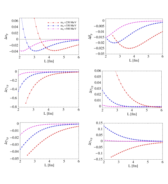
Figure 1: Volume dependence of the proton polarisabilities. Here we show the ratio of the difference of the finite and infinite volume results to the infinite volume results for three values of the pion mass using the parameters described in the text. The curves terminate at $m_{\pi}\ L=3$.

dependence of the various polarisabilities in the proton. Here we have specialised to QCD, and chosen physical values for the various constants. In the figure, we show results for the ratio $\Delta X(L)=[X(L)-X(\infty)]/X(\infty)$ for the six polarisabilities at three different pion masses, $m_{\pi}=0.25,\,0.35,\,0.50$ GeV. The overall magnitude of these shifts varies considerably; generally volume effects are at the level of 5–10% for $m_{\pi}=0.25$ GeV and smaller for larger masses. Larger effects are seen in a number of the spin polarisabilities but there are as yet no lattice calculations of these quantities. Results in Ref. [1] also allow us to calculate the finite volume effects in the quenched data on the various polarisabilities calculated in Refs. [4, 5]. The quenched expressions involve a number of undetermined LECs, so we can only estimate the volume effects. Using reasonable range for these parameters, we see that the calculations on a (2.4 fm)³ lattice with $m_{\pi}=$0.5 GeV may differ from their infinite volume values by 5–10% in the case of the electric polarisability.

4 Conclusion

We have investigated Compton scattering from spin-half targets from the point of view of lattice QCD. We first discussed how external field methods can be used to probe all six polarisabilities of real Compton scattering for both charged and uncharged targets. We also discussed the effects of the finite volume used in lattice calculations on the polarisabilities. Since polarisabilities are infrared-sensitive observables (they scale as inverse powers of the pion mass near the chiral limit), they are expected to have strong volume dependence. This is indeed borne out in the explicit calculations presented here. In QCD, we generically find that the polarisabilities experience volume shifts of 5–10% from the infinite volume values for lattice volumes $\sim$(2.4 fm)³ and pions of mass 0.25 GeV. In the case of quenched QCD (relevant to the only existing lattice data), we find significant effects even at pion masses $\sim 0.5$ GeV. Future lattice studies of the polarisabilities should take these effects into account in order to present physically relevant results.

- [1] W. Detmold, B. C. Tiburzi and A. Walker-Loud, Phys. Rev. D 73, 114505 (2006).
- [2] S. Ragusa, Phys. Rev. D 47, 3757 (1993).
- [3] H. R. Fiebig, W. Wilcox and R. M. Woloshyn, Nucl. Phys. B 324, 47 (1989).
- [4] J. Christensen, W. Wilcox, F. X. Lee and L. m. Zhou, Phys. Rev. D 72, 034503 (2005).
- [5] F. X. Lee, L. Zhou, W. Wilcox and J. Christensen, Phys. Rev. D 73, 034503 (2006).
- [6] S. Weinberg, Phys. Rev. Lett. 17, 616 (1966); J. Gasser and H. Leutwyler, Annals Phys. 158, 142 (1984); Nucl. Phys. B 250, 465 (1985).
- [7] F. Fucito, G. Parisi and S. Petrarca, Phys. Lett. B 115, 148 (1982).
- [8] G. Martinelli, G. Parisi, R. Petronzio and F. Rapuano, Phys. Lett. B 116, 434 (1982).
- [9] C. W. Bernard, T. Draper, K. Olynyk and M. Rushton, Phys. Rev. Lett. 49, 1076 (1982).
- [10] S. Aoki and A. Gocksch, Phys. Rev. Lett. 63, 1125 (1989) [Erratum-ibid. 65, 1172 (1990)]; S. Aoki, A. Gocksch, A. V. Manohar and S. R. Sharpe, Phys. Rev. Lett. 65, 1092 (1990).
- [11] E. Shintani et al., PoS LAT2005, 128 (2006).
- [12] W. Detmold, Phys. Rev. D 71, 054506 (2005).
- [13] D. Babusci, G. Giordano, A. I. L’vov, G. Matone and A. M. Nathan, Phys. Rev. C 58, 1013 (1998).
- [14] J. S. Schwinger, Phys. Rev. 82, 664 (1951).
- [15] J. Wess and B. Zumino, Phys. Lett. B 37, 95 (1971);
- [16] E. Witten, Nucl. Phys. B 223, 422 (1983).
- [17] T. R. Hemmert, B. R. Holstein, J. Kambor and G. Knochlein, Phys. Rev. D 57, 5746 (1998).
- [18] J. Gasser and H. Leutwyler, Phys. Lett. B 188, 477 (1987).
- [19] W. Detmold and M. J. Savage, Phys. Lett. B 599, 32 (2004).