Partially quenched QCD with a chemical potential

Abstract:

Using a chiral random matrix theory we can now derive the low energy partition functions and Dirac eigenvalue correlations of QCD with different chemical potentials for the dynamical and valence quarks. The results can also be extended to complex (and purely imaginary) chemical potential. We also discuss possible applications such as fitting to low energy constants and understanding the phase diagrams of the full and partially quenched theories.

1 Introduction

Since the work of Banks and Casher [1] it has been known that the low eigenvalues of the QCD Dirac operator are related to the breaking of chiral symmetry. Later Leutwyler and Smilga [2] showed that the low energy partition function for QCD was universal and could be determined directly from the finite volume chiral Lagrangian. This led to a set of sum rules for inverse powers of the Dirac eigenvalues. Shuryak and Verbaarschot [3] then discovered that these sum rules could also be obtained from a Random Matrix Theory (RMT) based on chiral symmetry. Thus the low eigenvalue spectrum of the RMT is also universal and agrees with QCD. By now this agreement has been extensively checked by lattice simulations.

Since the RMT results contain an explicit volume dependence one use for them has been to extract infinite volume results from finite volume lattice simulations. This was first done for the chiral condensate [4] since that was the only available parameter in the RMT. Since then it was realized that the low energy partition function of quenched QCD with a chemical potential also depends on the pion decay constant as does the eigenvalues [5]. The determination of exact results for the low eigenvalue distributions of quenched QCD with a chemical potential [6] has then provided one way to extract both constants in quenched lattice simulations [7]. The eigenvalue distributions for unquenched QCD are also know [8], but due to the complex action they are not practical for current simulations. One alternative that has been suggested is to use an imaginary isospin chemical potential [9]. Then the action is real and also a Hermitian eigensolver can still be used. However for the unquenched simulations this required generating lattices with an imaginary isospin chemical potential which, although it does not cause any complications, it is not generally done.

The ideal case is to consider partially quenched ensembles where the dynamical simulation is performed at one chemical potential (preferably zero) and the eigenvalues are extracted using a different (nonzero) chemical potential. We thus consider observables of the form

$$\langle O\rangle=\frac{1}{Z}\int d[A]~{}O(\makebox[0.0pt][l]{$\,/$}D(\mu_{0}))~{}\mathrm{e}^{-S_{g}(A)}\prod_{f=1}^{N_{f}}\det[\makebox[0.0pt][l]{$\,/$}D(\mu_{f})+m_{f}]$$ (1)

where $S_{g}$ is the gauge action and $\makebox[0.0pt][l]{$\,/$}D(\mu)$ is the Dirac operator with quark chemical potential $\mu$. If the observable only depends on the low energy (zero momentum) modes then the results are universal and can be evaluated using a chiral effective theory such as RMT. The observables we consider here are correlations of the Dirac eigenvalues so that

$$O(X)=\sum_{k}\delta^{2}(z_{1}-\lambda_{k}(X))~{}\left\{\sum_{\ell}\delta^{2}(z_{2}-\lambda_{\ell}(X))\ldots\right\}$$ (2)

with $\lambda_{k}(X)$ the complex eigenvalues of $X$. Partially quenched eigenvalue correlations with an imaginary isospin chemical potential have recently been published [10] and details of the calculation for a real chemical potential will appear elsewhere [11]. Here we present some details on the RMT used along with a sample of the results.

2 Dirac eigenvalues from partially quenched partition functions

One way to calculate correlations of Dirac eigenvalues is from the partially quenched partition functions

$$Z_{N_{f},N_{b}}(\{m_{f}|m_{b}\},\{\mu_{f}|\mu_{b}\})=\int d[A]\mathrm{e}^{-S_{g}(A)}\frac{\prod_{f=1}^{N_{f}}\det[\makebox[0.0pt][l]{$\,/$}D(\mu_{f})+m_{f}]}{\prod_{b=N_{f}+1}^{N_{f}+N_{b}}\det[\makebox[0.0pt][l]{$\,/$}D(\mu_{b})+m_{b}]}~{}.$$ (3)

The partially quenched eigenvalue density for one dynamical flavor, for example, is given by [12]

$$\rho_{1}(z,\mu_{0}|m_{1},\mu_{1})=\left[\frac{1}{\pi}\partial_{{\bar{z}}}\partial_{z}Z_{3,2}(\{m_{1},z,{\bar{z}}|m_{b},\bar{m}_{b}\},\{\mu_{1},\mu_{0},-\mu_{0}|\mu_{b},-\mu_{b}\})\right]_{m_{b}=z,\bar{m}_{b}=\bar{z},\mu_{b}=\mu_{0}}~{}.$$ (4)

The presence of the extra (conjugate) flavors with negative $\mu$ is required when the eigenvalue spectrum of the Dirac operator is complex. The necessary partition functions can then in principle be obtained from zero momentum chiral Lagrangians, however these are only known for certain cases. The purely fermionic partition function is given by [5]

$$Z_{N_{f},0}=\int_{U(N_{f})}dU\det(U)^{\nu}\exp\left(\frac{1}{2}\Sigma V\mathrm{Tr}\,M\{U+U^{\dagger}\}-\frac{1}{4}F^{2}V\mathrm{Tr}[U,Q][U^{\dagger},Q]\right)$$ (5)

where $\Sigma$ and $F$ are the tree level condensate and pion decay constant and $M$ and $Q$ are diagonal matrices of $m_{f}$ and $\mu_{f}$ respectively. The bosonic partition function $Z_{0,2}$ is also known [6]. So far no direct evaluation of a partially quenched chiral Lagrangian has been performed. Instead the partially quenched partition functions can now be evaluated from RMT.

3 RMT for QCD with a chemical potential

Here we will consider a variant of the RMT introduced in [8]. The Dirac matrix in a chiral basis is written as (for zero mass)

$$\mathcal{D}_{f}=\left(\begin{array}[]{cc}0&ia_{f}\Phi+b_{f}\Theta\\ ia_{f}\Phi^{\dagger}+b_{f}\Theta^{\dagger}&0\end{array}\right)~{}.$$ (8)

Here $\Phi$ and $\Theta$ are complex $(N+\nu)\times N$ matrices with $\nu$ the topological charge. We start with a more general form of the Dirac matrix where $a_{f}\equiv a(T,\mu_{f})$ and $b_{f}\equiv b(T,\mu_{f})$ are functions of the temperature and chemical potentials that we will determine next. The QCD partition function with $N_{f}$ quark flavors can now be modeled as

$$Z=\int d\Phi~{}d\Theta~{}\exp\left(-\alpha N\mathrm{Tr}\left[\Phi^{\dagger}\Phi+\Theta^{\dagger}\Theta\right]\right)\prod_{f=1}^{N_{f}}\det(\,\mathcal{D}_{f}+m_{f}\,)~{}.$$ (9)

The constant $\alpha$ sets the average eigenvalue spacing and will also be determined next. We could absorb it into $a$ and $b$, but instead will choose a normalization such that $a(T,\mu=0)=1$ and $b(T,\mu=0)=0$.

The coefficients can be determined by comparing to the chiral Lagrangian at nonzero $\mu$. The mapping follows very closely to that for $\mu=0$ given in [13]. First the fermion determinants are all written in terms of Grassmann variables as

$$\det(\mathcal{D}_{f}+m_{f})=\int d\bar{\psi}_{1,2}^{f}d\psi_{1,2}^{f}\exp\left[m_{f}\sum_{k}\bar{\psi}_{k}^{f}\psi_{k}^{f}+\bar{\psi}_{1}^{f}(ia_{f}\Phi+b_{f}\Theta)\psi_{2}^{f}+\bar{\psi}_{2}^{f}(ia_{f}\Phi^{\dagger}+b_{f}\Theta^{\dagger})\psi_{1}^{f}\right]~{}.$$ (10)

Then the Gaussian integration over the matrices $\Phi$ and $\Theta$ can be performed. The result is

$$Z\propto\int\prod_{f}d\bar{\psi}_{1,2}^{f}d\psi_{1,2}^{f}\exp\left[m_{f}\sum_{k}\bar{\psi}_{k}^{f}\psi_{k}^{f}+\sum_{g}\frac{a_{f}a_{g}-b_{f}b_{g}}{\alpha N}\bar{\psi}_{1}^{f}\psi_{1}^{g}\bar{\psi}_{2}^{g}\psi_{2}^{f}\right]~{}.$$ (11)

If we consider only a baryon chemical potential such that all flavors have the same chemical potential $\mu_{f}=\mu_{B}$, the coefficient of the four fermion term becomes $[a^{2}(T,\mu_{B})-b^{2}(T,\mu_{B})]/\alpha N$. At zero temperature we expect that the partition function does not depend on the baryon chemical potential. We can ensure this in the RMT by setting $a^{2}(0,\mu)-b^{2}(0,\mu)=1$. For nonzero temperature this will not be the case and one can leave the functions $a$ and $b$ independent. As was mentioned previously [14], this could possibly be used to help map out the QCD phase diagram.

A nonlinear sigma model is obtained by using a Hubbard-Stratonovitch transformation to break apart the four fermion terms and then integrate out the Grassmann variables. This gives

$$Z=\int d\sigma\,\mathrm{e}^{-\alpha N\mathrm{Tr}\sigma^{\dagger}\sigma}\det(\sigma+M)^{N+\nu}\det(\sigma^{\dagger}+P+M)^{N}$$ (12)

with $\sigma$ a $N_{f}\times N_{f}$ complex matrix and $P=A\sigma^{\dagger}A-B\sigma^{\dagger}B-\sigma^{\dagger}$ such that $P=0$ at $\mu_{f}=0$. We also define $A$, $B$ and $M$ to be the diagonal matrices of $a_{f}$, $b_{f}$ and $m_{f}$ respectively. For small $m_{f}$ and $\mu_{f}$ the determinants can be expanded as

$$\det(\sigma+M)^{N+\nu}\det(\sigma^{\dagger}+P+M)^{N} \approx \exp\left(N\mathrm{Tr}\left[\ln(\sigma^{\dagger}\sigma)+M\sigma^{-1}+(M+P)\sigma^{\dagger-1}\right]\right)~{}.$$ (13)

At $T=0$ we can also use the relation $A^{2}-B^{2}=1$ to expand $A$ as $A\approx 1+B^{2}/2$ which we will use below. For $m_{f}=0$ and $\mu_{f}=0$ the large $N$ saddle point is given by $\sigma^{\dagger}\sigma=1/\alpha$. Thus the Goldstone manifold is simply the unitary group [13]. The low energy partition function is then

$$\int dU\det(U)^{\nu}\exp\left(N\mathrm{Tr}\sqrt{\alpha}M\{U+U^{\dagger}\}-N\mathrm{Tr}[U,B][U^{\dagger},B]\right)~{}.$$ (14)

By matching terms with (5) we find that

$$\sqrt{\alpha} \approx \frac{\Sigma V}{2N}$$

$$b(T=0,\mu) \approx \mu F\sqrt{\frac{V}{2N}}$$

$$a(T=0,\mu) \approx 1+\mu^{2}F^{2}\frac{V}{4N}~{}.$$ (15)

With these definitions we then have a RMT that maps directly onto the zero momentum chiral Lagrangian. We note that the $O(\mu^{2})$ term in $a$ above only contributes to the overall normalization of the partition function. We can therefore neglect it for most observables. However quantities like the partition function, particle number and related susceptibilities will depend on it.

4 Partially quenched eigenvalue correlations

A nice feature of the above RMT is that the partition function can be rewritten directly in terms of the eigenvalues of the Dirac matrix (8). This was originally done for the unquenched model where the dynamical and valence chemical potentials are all the same [8]. It is also possible to do this for the partially quenched case, although the results become much more complicated. Due to space constraints we will only show plots of some of the results and save the details of the calculation for a future publication [11].

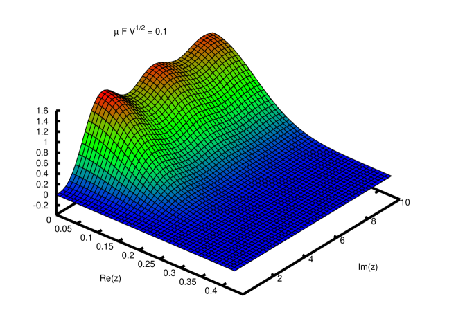
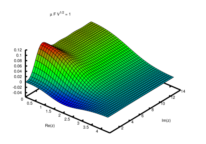
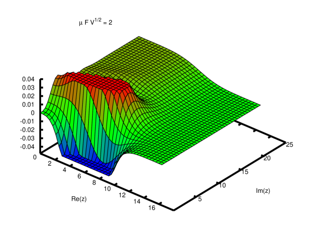
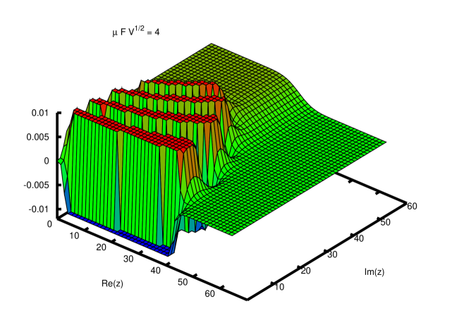
Figure 1: Real part of the one flavor eigenvalue density for dynamical mass $m=0$ at different chemical potentials $\mu$. The peaks have been clipped for better illustration at $\mu F\sqrt{V}=2,4$.

As a review we first show results for the one flavor eigenvalue density [8, 15]. In figure 1 we plot the real part of the density for dynamical mass $m=0$ for different values of the common chemical potential $\mu$. At $\mu=0$ the eigenvalues are purely imaginary. For small $\mu$ they begin to spread out into the complex plane, but still show the characteristic oscillations along the imaginary axis due to chiral symmetry. For larger $\mu$ those oscillations disappear and a new set of oscillations appear around the real axis. These oscillations grow exponentially with the volume and also change sign unlike the ones for small $\mu$. They are not seen in the quenched density and are in turn responsible for producing a nonzero chiral condensate [16].

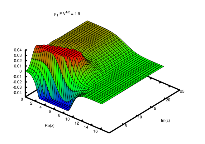
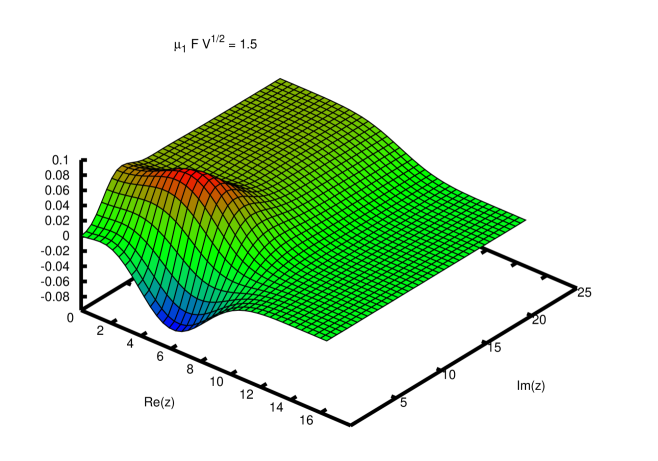
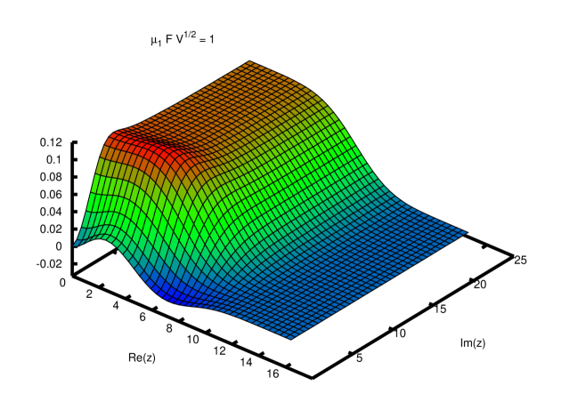
Figure 2: Real part of the partially quenched eigenvalue density for valence chemical potential $\mu_{0}F\sqrt{V}=2$ with dynamical mass $m_{1}=0$ and different dynamical chemical potentials $\mu_{1}$. The peak has been clipped for better illustration at $\mu_{1}F\sqrt{V}=1.9$.

We now start with the one flavor density at $\mu F\sqrt{V}=2$ and lower the dynamical chemical potential $\mu_{1}$ as the valence chemical is held fixed at $\mu_{0}=\mu$. This is show in figure 2. The peak that is seen near the real axis (which is clipped at $\mu_{1}F\sqrt{V}=1.9$) stays at about the same height as $\mu_{1}$ varies. However the background density increases filling in the valley along the real axis until the oscillations are completely covered at $\mu_{1}=0$. At this point the density looks more like the quenched density shown in figure 3 than the one flavor result. The main differences between the quenched and partially quenched in this case are the overall scale and the relative size of the “bump” along the real axis.

We can also extend these results to a complex chemical potential including a purely imaginary one. This could be used to test analytic continuation of quantities from imaginary to real chemical potentials. An imaginary chemical potential can also be used for fitting the low energy constants $\Sigma$ and $F$. However in this case it is better to consider the mixed eigenvalue correlation between a valence and dynamical eigenvalue [9, 10], since it is much more sensitive to the chemical potential.

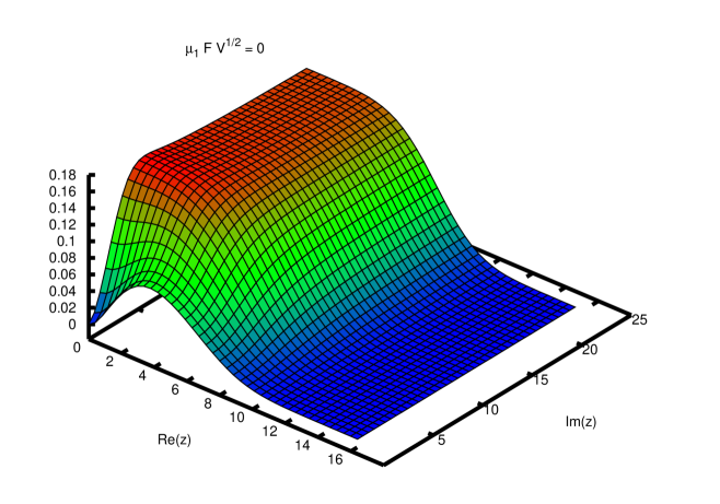
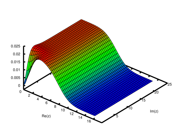
Figure 3: Partially quenched (left) and quenched (right) eigenvalue density for valence chemical potential $\mu_{0}F\sqrt{V}=2$. The dynamical chemical potential for the partially quenched is $\mu_{1}=0$ with dynamical mass $m_{1}=0$. Note the different scales.

5 Conclusions

We have shown results for the eigenvalue correlations of partially quenched QCD with different dynamical and valence chemical potentials. This could be useful for fitting low energy constants on existing lattices generated at zero chemical potential. It is also possible to generate the low energy partition functions with different chemical potentials for each flavor from these results. This could then be applied, for example, to study three flavor QCD. Additionally the extension of the RMT to include coefficients which are general functions of temperature and chemical potential may be useful for mapping out the QCD phase diagram.

References

- [1] T. Banks and A. Casher, Nucl. Phys. B 169, 103 (1980).
- [2] H. Leutwyler and A. Smilga, Phys. Rev. D 46, 5607 (1992).
- [3] E.V. Shuryak and J.J.M. Verbaarschot, Nucl. Phys. A 560, 306 (1993); J.J.M. Verbaarschot, Phys. Rev. Lett. 72, 2531 (1994).
- [4] M.E. Berbenni-Bitsch, A.D. Jackson, S. Meyer, A. Schäfer, J.J.M. Verbaarschot and T. Wettig, Nucl. Phys. Proc. Suppl. 63, 820 (1998); P.H. Damgaard, U.M. Heller and A. Krasnitz, Phys. Lett. B 445, 366 (1999).
- [5] D. Toublan and J.J.M. Verbaarschot, Int. J. Mod. Phys. B 15, 1404 (2001).
- [6] K. Splittorff and J.J.M. Verbaarschot, Nucl. Phys. B 683, 467 (2004).
- [7] J.C. Osborn and T. Wettig, PoS LAT2005, 200 (2005).
- [8] J.C. Osborn, Phys. Rev. Lett. 93, 222001 (2004).
- [9] P.H. Damgaard, U.M. Heller, K. Splittorff and B. Svetitsky, Phys. Rev. D 72, 091501 (2005); P.H. Damgaard, U.M. Heller, K. Splittorff, B. Svetitsky and D. Toublan, Phys. Rev. D 73, 074023 (2006); Phys. Rev. D 73, 105016 (2006).
- [10] G. Akemann, P.H. Damgaard, J.C. Osborn and K. Splittorff, [hep-th/0609059], submitted to Nucl. Phys. B.
- [11] G. Akemann, P.H. Damgaard, J.C. Osborn and K. Splittorff, in preparation.
- [12] V.L. Girko, Theory of random determinants (Kluwer Academic Publishers, Dordrecht, 1990); M.A. Stephanov, Phys. Rev. Lett. 76, 4472 (1996).
- [13] M.A. Halasz and J.J.M. Verbaarschot, Phys. Rev. D 52, 2563 (1995).
- [14] J.C. Osborn, Nucl. Phys. B (Proc. Suppl.) 140, 565 (2004).
- [15] G. Akemann, J.C. Osborn, K. Splittorff and J.J.M. Verbaarschot, Nucl. Phys. B 712, 287 (2005).
- [16] J.C. Osborn, K. Splittorff and J.J.M. Verbaarschot, Phys. Rev. Lett. 94, 202001 (2005).