First results with two light flavours of quarks with maximally twisted mass

Abstract:

We report on first results of an ongoing effort to simulate lattice QCD with two degenerate flavours of quarks by means of the twisted mass formulation tuned to maximal twist. By utilising recent improvements of the HMC algorithm, pseudo-scalar masses well below $300\,\mathrm{MeV}$ are simulated on volumes $L^{3}\cdot T$ with $T=2L$ and $L>2\,\mathrm{fm}$ and at values of the lattice spacing $a\lesssim 0.1\,\mathrm{fm}$. We present first evidence that scaling violations in the pseudo-scalar decay constant are small and well compatible with $\mathcal{O}(a)$ improvement. Additionally, exploratory results for the case of $N_{f}=2+1+1$ flavours are discussed.

1 Introduction

Originally, the twisted mass formulation of lattice QCD [1, 2] was invented to provide the Wilson lattice Dirac operator with an infra-red cut-off for its eigenvalue spectrum in order to prevent the appearance of unphysically small eigenvalues when the quark masses become small. More recently, however, another quite astonishing property of twisted mass quarks has been discovered: in Ref. [3] it was shown that pure Wilson twisted mass fermions lead to automatic $\mathcal{O}(a)$ improvement when tuned to full twist even without any improvement term added to the action.

In simulations in the quenched approximation it has been demonstrated that the presence of the twisted mass term as an infra-red regulator is indeed a clear advantage when compared to the pure Wilson regularisation [4]. However, this infra-red regulator appears, somewhat surprisingly, not to be crucial in simulations with light dynamical quarks. Here simulations even with standard Wilson fermions at pseudo-scalar masses below $300\,\mathrm{MeV}$ are possible, at least when newer algorithmic techniques are used, see e.g. our own work of Ref. [5].

It appears therefore that for the case of dynamical simulations the aforementioned automatic $\mathcal{O}(a)$ improvement of the (maximally twisted) Wilson formulation of lattice QCD becomes more important. In such a set-up only one parameter needs to be tuned in order to obtain $\mathcal{O}(a)$ improvement and there are no additional operator-specific improvement terms needed. Moreover, mixing patterns during renormalisation are greatly simplified.

The disadvantage of the twisted mass formulation is the fact that the twisted mass term explicitly breaks parity and flavour symmetry. The flavour symmetry breaking for instance introduces a mass splitting between the lightest charged and the uncharged pseudo-scalar mesons. However, all those effects stem only from the valence quark sector [6] (the sea quark determinant is flavour blind), are expected to be lattice artifacts of order $\mathcal{O}(a^{2})$. In particular, in a mixed action set-up, with for instance overlap valence fermions no breaking of parity or flavour chiral symmetry is expected.

In the quenched approximation it is by now established that automatic $\mathcal{O}(a)$ improvement works very well in practice [4, 7, 8, 9, 10] . Also, the theoretical expectation of $\mathcal{O}(a^{2})$ lattice artifacts appearing in the pseudo-scalar mass splitting has been confirmed [11, 12]. In this proceeding contribution we will provide first evidence that maximally twisted mass quarks are $\mathcal{O}(a)$ improved also in dynamical simulations and that the residual $\mathcal{O}(a^{2})$ lattice artifacts are small. The lowest value of the pseudo-scalar mass covered in these simulations is significantly below $300\,\mathrm{MeV}$, which is in a region where it is possible to confront the simulation data with chiral perturbation theory ($\chi$PT) and determine therefore the validity range of $\chi$PT. Since simulations directly at the physical value of the pion mass are still somewhat too expensive, $\chi$PT could then be used to bridge the gap between the simulation data and the physical point. The low values of the pseudo-scalar mass reached in our work became possible only due to recent algorithmic developments [13, 14, 15, 16, 5, 17, 18, 19] (See also the contribution by M. Clark to these proceedings). In particular, for all the $N_{f}=2$ results reported in this proceeding contribution we have used our variant of the HMC algorithm described in Ref. [5].

In addition to observables like pseudo-scalar mass and decay constant we will provide also first results for the aforementioned mass splitting in the pseudo-scalar sector and discuss the case of $N_{f}=2+1+1$ flavours of quarks, i.e. taking the strange and the charm quark into account in the simulation. For recent summaries of the status of Wilson twisted mass fermions see Refs. [20, 21], the review of Ref. [22] and references therein.

2 Choice of Lattice Action

The fermionic lattice action for two flavours of mass degenerate Wilson twisted mass quarks reads (in the so called twisted basis $\chi$)

$$\begin{split}S_{\mathrm{tm}}=\ a^{4}\sum_{x}\biggl{\{}&\bar{\chi}_{x}[am_{0}+4r+i\gamma_{5}\tau_{3}a\mu]\chi_{x}\Bigr{.}\\ &\Bigl{.}+\sum_{\nu=1}^{4}\bar{\chi}_{x}\left[U_{x,\nu}(r+\gamma_{\nu})\chi_{x+\hat{\nu}}+U_{x-\hat{\nu},\nu}^{\dagger}(r-\gamma_{\nu})\chi_{x-\hat{\nu}}\right]\biggr{\}}\,,\end{split}$$ (1)

where $am_{0}$ is the bare untwisted quark mass and $a\mu$ the bare twisted mass. $\tau_{3}$ is the third Pauli matrix acting in flavour space and $r$ is the Wilson parameter, which we set to one in our simulations.

Twisted mass fermions are said to be at maximal twist if the bare untwisted mass is tuned to its critical value $m_{\mathrm{crit}}$. We will discuss later on how this can be realised in practice.

In the gauge sector we use the so called tree-level Symanzik improved gauge action (tlSym) [23], which includes besides the plaquette term $U_{\Box}$ also rectangular $(1\times 2)$ Wilson loops $U^{1\times 2}_{x,\mu,\nu}$

$$S_{g}=\beta\sum_{x}\Biggl{(}b_{0}\sum_{1\leq\mu<\nu;\mu,\nu=1}^{4}\frac{1}{3}\{1-\operatorname{Re}\operatorname{Tr}(U_{\Box})\}\Bigr{.}\Bigl{.}\ +\ b_{1}\sum_{\mu\neq\nu;\mu,\nu=1}^{4}\frac{1}{3}\{1-\operatorname{Re}\operatorname{Tr}(U^{1\times 2}_{x,\mu,\nu})\}\Biggr{)}\,,$$ (2)

with the bare inverse coupling $\beta$, $b_{1}=-1/12$ and the normalisation condition $b_{0}=1-8b_{1}$. Note that with $b_{1}=0$ this action corresponds to the usual Wilson plaquette action.

Before presenting the actual results let us first briefly recall some earlier works which led to the present production set-up, see also Ref. [20]. As mentioned before, in the quenched approximation we have shown in an extended scaling test that $\mathcal{O}(a)$ improvement works extremely well for maximally twisted mass quarks [4, 7, 8]. In the context of this scaling test also several definitions for full twist were examined and it was found that in agreement with theoretical considerations [24, 25, 26] the so called PCAC definition leads to small residual lattice artifacts of $\mathcal{O}(a^{2})$ in the whole range of – in particular, also small – masses investigated: for the PCAC definition, at a fixed value of $a\mu>0$, $am_{\mathrm{crit}}$ is determined from the condition that

$$m_{\mathrm{PCAC}}=\frac{\sum_{\mathbf{x}}\langle\partial_{0}A_{0}^{a}(x)P^{a}(0)\rangle}{2\sum_{\mathbf{x}}\langle P^{a}(x)P^{a}(0)\rangle}\qquad a=1,2$$ (3)

vanishes for large enough time separation such that a projection on the pion state is reached. This provides then $am_{\mathrm{crit}}$ as a function of $a\mu$ and the final value of $am_{\mathrm{crit}}$ may be obtained by (linearly) extrapolating $am_{\mathrm{crit}}(\mu)$ to $\mu=0$. However, the extrapolation of $am_{\mathrm{crit}}(\mu)$ to $\mu=0$ is not necessary: taking the value of $am_{\mathrm{crit}}$ at the lowest value of $a\mu$ that is used in the simulation is an equally good definition. This remark is of particular importance for dynamical simulations where one might not be able to afford to determine $am_{\mathrm{crit}}$ at several values of $a\mu$ and then perform the extrapolation to $\mu=0$.

Furthermore, in the dynamical case it is not clear at all how an extrapolation to $a\mu=0$ could be performed: a generic property of Wilson type fermions is its non-trivial phase structure at finite lattice spacing with first order phase transitions close to the chiral limit, which was investigated in detail by means of twisted mass fermions in Refs. [27, 28, 29, 20] and which is in accordance with the picture developed in $\chi$PT [30, 31]. A very important consequence of this phenomenon is that at a non-vanishing lattice spacing the value of the pseudo-scalar mass cannot drop below a certain minimal value without being affected by the first order phase transition. From the analysis in $\chi$PT it is expected that the corresponding minimal value of the twisted mass parameter goes to zero proportional to $a^{2}$ towards the continuum limit. Hence, one can always find a largest value of the lattice spacing $a_{\mathrm{max}}$ where simulations with a given value of the pseudo-scalar mass can be performed.

The actual value of $a_{\mathrm{max}}$ depends on many details, for instance on the gauge action used in the simulation. For example, when the Wilson plaquette gauge action is used one can estimate $a_{\mathrm{max}}\approx 0.07-0.1\,\mathrm{fm}$ to realise a pseudo-scalar mass of $250\,\mathrm{MeV}$. The situation improves, when also the $2\times 1$ rectangular loops are included (see Eq. (2)): the value of $a_{\mathrm{max}}$ increases when the modulus of the coefficient $b_{1}$ multiplying the rectangular part is increased [29, 28]. The study of different gauge actions led us to the conclusion that the tlSym gauge action, with a coefficient of $b_{1}=-1/12$, is a good choice to avoid on the one hand large effects related to the presence of the phase transition and on the other hand the possible conceptual issues concerning the DBW2 gauge action, with coefficient $b_{1}=-1.4088$, [20].

3 Set-up and First Results

$\Bigl{.}\Bigr{.}\beta$	$L^{3}\times T$	$a\mu_{\mathrm{min}}$	$\kappa_{\mathrm{crit}}(a\mu_{\mathrm{min}})$	$r_{0}/a(a\mu_{\mathrm{min}})$
$3.9$	$24^{3}\times 48$	$0.004$	$0.160856$	$5.184(41)$
$4.05$	$32^{3}\times 64$	$0.003$	$0.15701$	$6.525(101)$

Table 1: The parameters for the simulation. We denote by $a\mu_{\mathrm{min}}$ the smallest value of the twisted mass parameter $a\mu$ at which we have performed simulations. At this value of $a\mu$ we determined the critical mass $m_{\mathrm{crit}}$, or, equivalently the hopping parameter $\kappa_{\mathrm{crit}}=1/(8+2am_{\mathrm{crit}})$. In order to convert to physical units, we take the value of $r_{0}/a$ as computed at $a\mu_{\mathrm{min}}$.

The main goal of the present work is to investigate, whether also in the case of $N_{f}=2$ mass-degenerate flavours of dynamical quarks, the lattice artifacts are as small as has been found in the quenched approximation when maximally twisted Wilson fermions are used. The current status of our simulations are summarised in tables 1 and 2. While in table 1 we provide the parameters of our simulations, in table 2 we also give current estimates of the pseudo-scalar mass $m_{\mathrm{PS}}$ in physical units, where we used $r_{0}=0.5\,\mathrm{fm}$. In addition we provide the number of equilibration trajectories $N_{\mathrm{therm}}$, the current statistics $N_{\mathrm{traj}}$ we have available and estimates of the integrated plaquette autocorrelation time where available.

The algorithm we used is a HMC algorithm with mass preconditioning [13] and multiple time scale integration. It is described in detail in Ref. [5]. The trajectory length was set to $1/2$ in all our runs. Our currently available estimates of the plaquette integrated autocorrelation time $\tau_{\mathrm{int}}(P)$ quoted in table 2 are in units of $\tau=1/2$.

$\Bigl{.}\Bigr{.}\beta$	$a\mu$	$m_{\mathrm{PS}}\,[\mathrm{MeV}]$	$N_{\mathrm{therm}}$	$N_{\mathrm{traj}}$	$\tau_{\mathrm{int}}(P)$
$3.9$	$0.0040$	$280$	$1500$	$5000$	$55(17)$
	$0.0064$	$350$	$1500$	$5000$	$23(07)$
	$0.0100$	$430$	$1500$	$5000$	$15(04)$
	$0.0150$	$530$	$1500$	$5000$	$06(02)$
$4.05$	$0.0030$	$266$	$1500$	$2200$	-
	$0.0060$	$372$	$1500$	$500$	-

Table 2: Current status of the simulations at $\beta=3.9$ and $\beta=4.05$ using the simulation parameters listed in table 1. In addition we give the current estimates of $m_{\mathrm{PS}}$ in physical units ($r_{0}=0.5\,\mathrm{fm}$) and of $\tau_{\mathrm{int}}(P)$ where available.

Full twist is realised in our simulations by tuning at a fixed value of $\beta$ the PCAC quark mass $m_{\mathrm{PCAC}}$ to zero at the smallest value $a\mu_{\mathrm{min}}$ of the twisted mass parameter $a\mu$. Keeping then the value of $\kappa_{\mathrm{crit}}$ or, equivalently, $m_{\mathrm{crit}}$, for all the other values of $a\mu$ provides $\mathcal{O}(a)$ improvement for all relevant physical quantities (see Refs. [25, 24, 8]). We list in table 1 the values of $\kappa_{\mathrm{crit}}$ which we then kept fixed for all simulations at a given value of $\beta$. The dependence of $am_{\mathrm{PCAC}}$ on $a\mu$ is shown in figure 1(a). The fact that at values of $a\mu>a\mu_{\mathrm{min}}$ the PCAC quark mass $am_{\mathrm{PCAC}}$ does not vanish will only lead to effects that are of $\mathcal{O}(a^{2})$ and hence will not destroy $\mathcal{O}(a)$ improvement.

In order to make maximum use of the gauge configurations, we evaluate connected meson correlators using a stochastic method to include all spatial sources. This method involves a stochastic source (Z(2)-noise in both real and imaginary part) for all colours and spatial locations at one Euclidean time slice. By solving for the propagator from this source for each of the 4 spin components, we can construct zero-momentum meson correlators from any quark bilinear at the source and sink. This method involves 4 inversions per Euclidean time slice value selected since we chose to use only one stochastic sample. This ”one-end” method is similar to that pioneered in Ref. [32] and implemented in Ref. [33]. We also employ a fuzzed source [34] of extent 6 lattice spacings to enable study of non-local meson creation and destruction operators.

In general, we save a gauge configuration every second trajectory and analyse meson correlators as described above from a selection of different Euclidean time slice sources. To reduce autocorrelations, we only use the same time slice source every 8-10 trajectories. Our primary statistical error analysis is from a bootstrap analysis of blocks of configurations. This estimate was cross-checked by varying the block size.

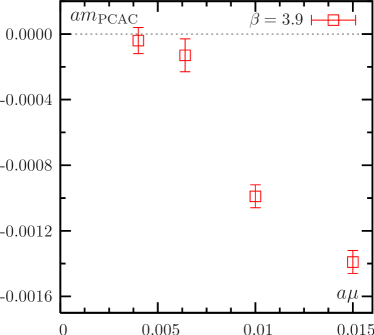
(a) $am_{\mathrm{PCAC}}$ as a function of $a\mu$ at $\beta=3.9$.

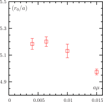
(b) $r_{0}$ as a function of $a\mu$ at $\beta=3.9$.

Figure 1: PCAC quark mass and Sommer parameter as a function of the twisted mass.

3.1 Setting the Scale

As mentioned already we used for this first analysis the Sommer parameter $r_{0}$ with a value of $0.5\,\mathrm{fm}$ to set the scale. While $r_{0}/a$ is measurable to high accuracy in lattice QCD simulations it has the drawback that its value in physical units is not known very well, which might introduce a non-negligible uncertainty. Therefore, it could be advantageous to determine the scale using other quantities which are experimentally better known, such as $f_{\pi}$, $f_{\mathrm{K}}$ or $m_{\mathrm{K}^{*}}$ which we plan to do in the future.

In figure 1(b) we plot $r_{0}/a$ as a function of $a\mu$ at $\beta=3.9$. Within the current errors the mass dependence of this quantity seems to be rather weak for the lowest three values of $a\mu$ , which would allow for a constant extrapolation to the physical point ($m_{\pi}=137\,\mathrm{MeV}$). Again, for the time being, we use the value of $r_{0}/a$ listed in table 1 determined at the value of $a\mu_{\mathrm{min}}$ as an estimate for $r_{0}/a$ at the physical point.

3.2 $f_{\mathrm{PS}}$, $m_{\mathrm{PS}}$ and other observables

In this subsection we present first results for $f_{\mathrm{PS}}$ and $m_{\mathrm{PS}}$. The pseudo-scalar mass $m_{\mathrm{PS}}$ is as usual extracted from the exponential decay of corresponding correlators constructed from local operators. In contrast to pure Wilson fermions, for maximally twisted mass fermions an exact lattice Ward identity allows to extract the pseudo-scalar decay constant $f_{\rm PS}$ from the relation

$$f_{\mathrm{PS}}=\frac{2\mu}{m_{\mathrm{PS}}^{2}}|\langle 0|P^{1}(0)|\pi\rangle|\,,$$ (4)

with no need of computing any renormalization constant since it turns out that $Z_{P}=1/Z_{\mu}$ [2].

In order to account for finite size (FS) effects in $m_{\mathrm{PS}}$ and $f_{\mathrm{PS}}$ we used NLO $\chi$PT formulae as derived by Gasser and Leutwyler [35]. The corrections decrease exponentially with a rate $m_{\mathrm{PS}}\cdot L$ (which we take from our data) and are proportional to the overall factor $(f_{\mathrm{PS}}\cdot L)^{-2}$. The quantity $f_{\mathrm{PS}}\cdot L$ is estimated at the chiral point either via extrapolation of uncorrected data for $f_{\mathrm{PS}}$ or from the phenomenological value of $f_{\pi}$ assuming $r_{0}=0.5\,\mathrm{fm}$. The difference between the results for the corrected $f_{\mathrm{PS}}$ obtained in the two ways at the physical point is about $0.4\,\mathrm{MeV}$, which is certainly less than the uncertainty arising from neglecting higher orders in $\chi$PT for the FS effects. Using the socalled re-summed Lüscher formulae with NNLO $\chi$PT input (more precisely the data in Tables 3 and 4 of Ref. [36]), we obtained for $af_{\mathrm{PS}}$ estimates of the finite size correction factors that are very similar to those coming from simple NLO $\chi$PT, while for $am_{\mathrm{PS}}$ the Lüscher formula leads to somewhat larger corrections. Note that for a definite statement about FS corrections, simulations with larger lattices would be needed in order to cross-check the $\chi$PT predictions. Such simulations are in progress.

In figure 2(a) we show $(r_{0}m_{\mathrm{PS}})^{2}$ (not FS corrected) as a function of the twisted mass $r_{0}\mu$ for the two $\beta$-values available. The dependence is to a very good approximation linear in $r_{0}\mu$ and the data at the two $\beta$ values fall approximately on a common line. Note that the renormalization factor $Z_{\mu}$ has not been taken into account here. The dotted line is not a fit to the data, but a line connecting the highest data point in $r_{0}\mu$ of $\beta=3.9$ with the origin and may serve to guide the eye.

In figure 2(b) $af_{\mathrm{PS}}$ is plotted versus $(am_{\mathrm{PS}})^{2}$ at $\beta=3.9$ only. In the plot we give the FS corrected and uncorrected data. Clearly, the effect of the FS correction is visible but not huge. In any case, whether we perform a FS correction or not the data show a curvature. It is very tempting to perform a fit of the data according to the expectation from $\chi$PT. For this, it would, however, be better to have a simulation at an additional value of $a\mu>a\mu_{\mathrm{min}}$. Such a simulation is presently in progress and we will report the results in a forthcoming publication [37].

A linear extrapolation of the FS corrected data of $f_{\mathrm{PS}}$ at $\beta=3.9$ towards the physical point ($m_{\pi}=137\,\mathrm{MeV}$) yields a value of $f_{\pi}=129.0\pm 0.5\pm 1.0\,\mathrm{MeV}$ (to be compared with $f_{\pi}=131\,\mathrm{MeV}$). The first error comes from the errors on $f_{\mathrm{PS}}$, $m_{\mathrm{PS}}$ and the extrapolation in the quark mass, the second from the uncertainty on the value of $r_{0}/a$. Systematic errors due to lattice artifacts, residual finite volume effects and the choice of $r_{0}=0.5\ \mathrm{fm}$ are not included.

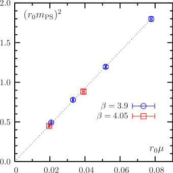
(a) $(r_{0}m_{\mathrm{PS}})^{2}$ as a function of $r_{0}\mu$ at $\beta=3.9$ and $\beta=4.05$.

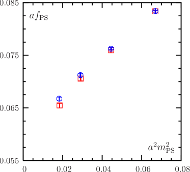
(b) $af_{\mathrm{PS}}$ as a function of $(am_{\mathrm{PS}})^{2}$ at $\beta=3.9$ without (squares) and with (circles) FS correction.

Figure 2: $(r_{0}m_{\mathrm{PS}})^{2}$ as a function of $r_{0}\mu$ for both $\beta$ values and $af_{\mathrm{PS}}$ as a function of $(am_{\mathrm{PS}})^{2}$ for $\beta=3.9$ only.

In figure 3 we show a comparison of quenched and dynamical values of the average momentum $\langle x\rangle$ corresponding to the expectation value of a non-singlet operator in pion states. Although the data point from the dynamical simulation still has systematic uncertainties such as missing non-perturbative renormalisation and lack of a continuum extrapolation, the message of the graph is very encouraging: employing twisted mass fermions, it is clearly possible to address the approach to the physical point also for more complicated quantities than $m_{\mathrm{PS}}$ and $f_{\mathrm{PS}}$ . In addition it seems that such quantities can be computed rather precisely.

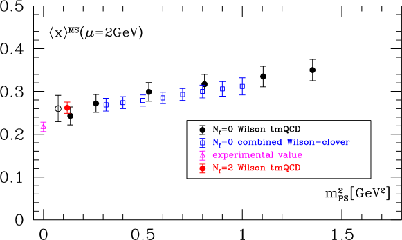
Figure 3: The average momentum of a parton in a pion. The blue squares correspond to quenched simulations [38] using the Schrödinger functional. These simulations have controlled non-perturbative renormalisation, finite volume effects and continuum limit. The black filled circles come from quenched calculations of the same quantity with maximally twisted Wilson fermions showing that with this approach much smaller quark masses can be reached, from Ref. [39] (the open circle corresponds to a point where finite size effects may possibly still affect the data). The red filled circle represents a simulation point obtained with dynamical quarks at $\beta=3.9$ (here the quenched renormalisation factor is used). Although a number of systematic effects, continuum limit and non-perturbative renormalisation still have to be analysed, it is to be noted that also at small quark masses dynamical results seem to agree with quenched ones.

3.3 Effects of Isospin Breaking

As mentioned before, a very important issue to address is the effect of isospin breaking in the twisted mass formulation at finite lattice spacing. This effect is expected to be most significant in the mass splitting between the lightest charged and uncharged pseudo-scalar mesons. A first analysis at $\beta=3.9$ and $a\mu=0.004$, taking the disconnected contribution in the neutral channel fully into account, shows that the uncharged pseudo-scalar meson is about $25\%$ lighter than the charged one. We get, in fact

$$am_{\pi}^{\pm}=0.1361(5)\,,\qquad am_{\pi}^{0}=0.103(4)\,,$$

or, expressed differently, $r_{0}^{2}((m_{\pi}^{0})^{2}-(m_{\pi}^{+})^{2})=c(a/r_{0})^{2}$ with $c\approx-5$, which has a magnitude that is a factor of 2 smaller than what was found in our quenched investigations [12]. Taking the value of $c=-5$ and assuming a linear dependence of the charged and neutral pseudo-scalar mass-squared on $a\mu$, we can compute the value of $a\mu$ where the neutral pion becomes massless and the phase transition line starts. This critical value would be $a\mu_{c}\simeq 0.0015$ at $\beta=3.9$ and hence well below the smallest value of $a\mu$ employed in our simulations. If we consider the mass splitting in the vector meson sector, we find that this splitting is compatible with zero within our currently still large errors. Note that the uncharged pion being lighter than the charged one is compatible with predictions from $\chi$PT [40] in case the first order phase transition scenario is realised.

Let us mention that the disconnected correlations needed for the $\pi^{0}$ meson are evaluated using a stochastic (Gaussian) volume source with 4 levels of hopping-parameter variance reduction [41]. We use 24 stochastic sources per gauge configuration and evaluate every $10$ trajectories.

3.4 Continuum Scaling of $f_{\mathrm{PS}}$

In figure 4 we show the scaling behaviour of $r_{0}f_{\mathrm{PS}}$ with $(a/r_{0})^{2}$ using our current simulation data. These results shown in the plot are still affected by some uncertainties: First of all the values of $r_{0}m_{\mathrm{PS}}$ are not (exactly) matched because there are only two values of $a\mu$ available at $\beta=4.05$. Second, we have taken – as mentioned before – the value of $r_{0}/a$ at $a\mu_{\mathrm{min}}$ at the two $\beta$-values as an estimate of the value at the physical point.

However, we do not believe that those uncertainties are larger than the current statistical uncertainty. Therefore, figure 4 suggests that lattice artifacts are rather small in $r_{0}f_{\mathrm{PS}}$ at the current level of accuracy. This result is a first indication that lattice artifacts are small and well under control in simulations with maximally twisted mass fermions, although further tests are clearly needed.

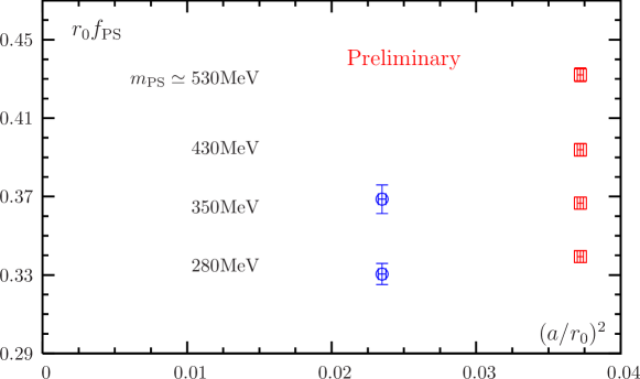
Figure 4: Preliminary scaling plot of $r_{0}f_{\mathrm{PS}}$ with $(a/r_{0})^{2}$. We also quote our current estimates of $m_{\mathrm{PS}}$ in physical units at $\beta=3.9$.

4 Including Strange and Charm Quarks

Adding to a doublet of mass-degenerate twisted mass quarks the strange quark can be realised in two possible ways. Either, a single quark flavour is introduced, or, a non-degenerate doublet of quarks is taken, as suggested in Ref. [42]. We have followed the prescription of Ref. [42] where it has been shown that a real quark determinant with a mass-split doublet can be obtained if the mass splitting term is taken to be orthogonal in isospin space to the twist direction. The reason for choosing this solution is that we want to realise $\mathcal{O}(a)$ improvement also for the non-degenerate case by using maximally twisted Wilson fermions. In this way, again no further improvement coefficients have to be computed.

The action for the non-degenerate quarks can be written in a form obtained from the physical basis of Ref. [42] by means of a chiral rotation around the direction 1 in isospin space to undo the twist of the Wilson term. The mass terms become

$$S_{m,2+1+1}=a^{4}\sum_{x}\big{\{}\bar{\psi}(x)[\tilde{m}_{0}+\mu_{\delta}\tau^{3}+i\mu_{\sigma}\gamma_{5}\tau^{1}]\psi(x)\big{\}}$$ (5)

where $\tilde{m}_{0}$ has again to be set to its critical value. In this case the renormalised current mass of the two quarks is given by $(\mu_{\sigma}/Z_{P}\pm\mu_{\delta}/Z_{S})$, where $Z_{P}$ and $Z_{S}$ are the renormalisation constans of the pseudo-scalar and scalar non-singlet operators (in the twisted basis). The $\psi$-fields couple to the gauge fields through the same Wilson-Dirac operator as the one of Eq. (1).

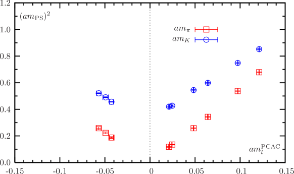
Figure 5: The squared pseudo-scalar pion and kaon masses as a function of the PCAC mass $am_{l}^{PCAC}$ of the light doublet ($a\mu_{l}=0.0075,a\mu_{\sigma}=0.2363,a\mu_{\delta}=0.2138$, $16^{3}\times 32$ lattices with tlSym gauge action, $\beta=3.35$). Owing to the presence of meta-stabilities, there is a gap between positive and negative values of $am_{l}^{PCAC}$. This implies a positive minimal value of the pion mass.

In our Monte Carlo simulations we described the $u$ and $d$ quarks by a light mass-degenerate twisted mass doublet and the $c$ and $s$ quarks by a heavy non-degenerate twisted mass doublet. We used the PHMC updating algorithm [43] with multi-step polynomial approximation and stochastic correction in the update chain as described in Refs. [44, 45].

As has been discussed in Refs. [6, 42, 46], in order to realise $\mathcal{O}(a)$ improvement, tuning to full twist can be achieved by setting the values of $\kappa_{c}$ of the light and heavy doublet equal. Therefore with respect to the $N_{f}=2$ simulations, we are left with only one additional parameter, i.e. the strange quark mass to be determined by the value of the kaon mass, while the charm quark is taken to be much heavier. In Ref. [46] we give a detailed discussion of possible ways to determine the twist angle, renormalisation factors and meson masses.

We find that simulations of $N_{f}=2+1+1$ dynamical quarks are feasible in practice. The tuning effort is similar to the $N_{f}=2$ case, modulo the need to know the ratio $Z_{P}/Z_{S}$ to fix the strange quark mass, and turns out to be possible without too much effort. Employing the tlSym gauge action as before, we find for lattice spacings as coarse as $a\approx 0.15\,$fm again signs of a first order phase transition which appears to be somewhat stronger than in the case of $N_{f}=2$ degenerate quarks. As a consequence of this phase transition the minimal pion mass cannot be made to vanish. This is illustrated in fig. 5. Nevertheless, our simulations allow to estimate the values of $\beta$ and $\mu$ where the lattice spacing is, say, $a\simeq 0.1\,{\rm fm}$ and safe simulations with a pion mass below $300\,{\rm MeV}$ become possible. $\chi$PT formulae for the case of non-degenerate quarks have already been developed [47] and have been confronted to our simulation results, see Ref. [46] for a discussion of this point.

5 Discussion

In this proceeding contribution we presented the status of an ongoing project to simulate two flavour lattice QCD with light maximally twisted mass quarks. Our first results are very encouraging.

• We reach a pseudo-scalar mass of $280\,\mathrm{MeV}$ (setting the scale with $r_{0}=0.5\,\mathrm{fm}$) while the simulation is performing smoothly and stable.

• Comparing results at 2 values of the lattice spacing, we find very good scaling, indicating that $\mathcal{O}(a)$ improvement is at work and that also the $\mathcal{O}(a^{2})$ lattice artifacts are small. This is in full accordance with earlier results in the quenched approximation.

• We do see effects of isospin breaking which are most significant in the mass splitting of the neutral and charged pions and turn out to be 25%. This is already much smaller than the corresponding splitting obtained in the quenched approximation. Note that at our smaller value of the lattice spacing, corresponding to $\beta=4.05$, the splitting would be at the 10% level only, if we assume an $a^{2}$ dependence of this effect as has been found in the quenched approximation.

• We have performed first simulations with non-degenerate strange and charm quark flavours in addition to the mass degenerate light doublet. It turns out that tuning and, in particular realising maximal twist, in this case is not problematic and needs a similar effort as other approaches taking the strange quark into account. We have explored the phase structure in this case and determined those parameters where simulations would not be affected by unwanted (first order) phase transitions. Hence, calculations with twisted mass and $N_{f}=2+1+1$ flavours are well prepared.

It has to be said that tuning to full twist has to be performed on the same large lattice as used later for the calculation of physical quantities. The reason for this is that we need to project to the pion state as fully as possible to determine the PCAC quark mass without being affected by finite size effects or excited state contributions. Thus the tuning itself is rather expensive. But, it only has to be done once, as it is the case for the determination of action improvement coefficients in other approaches. Note, however, that with twisted mass fermions we do not have to compute further operator specific improvement coefficients afterwards.

Our ongoing efforts concern the completion of the simulations at $\beta=3.9$ with an additional value of $a\mu$, which will be presented in a forthcoming publication [37]. The main thrust of the future work is to add another and finer value of the lattice spacing (and, maybe, also a coarser one). In this proceeding contribution we reported already about some first results in this direction which indicate only small scaling violations. Our large set of configurations is uploaded to the ILDG [48, 49] and will be used for computations of more complicated physical quantities than discussed here. Another interesting direction we follow with the twisted mass approach is to use Osterwalder-Seiler or overlap fermions in the valence sector [50] and to perform simulations at non-vanishing temperature on which first results were presented at this conference [51].

Acknowledgements

We thank NIC and the computer centres at Forschungszentrum Jülich and Zeuthen for providing the necessary technical help and computer resources. Computer time on UKQCD’s QCDOC in Edinburgh [52] using the Chroma code [53] and on apeNEXT [54] in Rome and Zeuthen and on MareNostrum in Barcelona (www.bsc.es) are gratefully acknowledged. This work has been supported in part by the DFG Sonderforschungsbereich/Transregio SFB/TR9-03 and the EU Integrated Infrastructure Initiative Hadron Physics (I3HP) under contract RII3-CT-2004-506078. We also thank the DEISA Consortium (co-funded by the EU, FP6 project 508830), for support within the DEISA Extreme Computing Initiative (www.deisa.org).

References

- [1] R. Frezzotti, P. A. Grassi, S. Sint and P. Weisz, A local formulation of lattice QCD without unphysical fermion zero modes, Nucl. Phys. Proc. Suppl. 83 (2000) 941–946 [hep-lat/9909003].
- [2] ALPHA Collaboration, R. Frezzotti, P. A. Grassi, S. Sint and P. Weisz, Lattice QCD with a chirally twisted mass term, JHEP 08 (2001) 058 [hep-lat/0101001].
- [3] R. Frezzotti and G. C. Rossi, Chirally improving Wilson fermions. I: O(a) improvement, JHEP 08 (2004) 007 [hep-lat/0306014].
- [4] L F Collaboration, K. Jansen, A. Shindler, C. Urbach and I. Wetzorke, Scaling test for Wilson twisted mass QCD, Phys. Lett. B586 (2004) 432–438 [hep-lat/0312013].
- [5] C. Urbach, K. Jansen, A. Shindler and U. Wenger, HMC algorithm with multiple time scale integration and mass preconditioning, Comput. Phys. Commun. 174 (2006) 87–98 [hep-lat/0506011].
- [6] R. Frezzotti and G. C. Rossi, Twisted-mass lattice QCD with mass non-degenerate quarks, Nucl. Phys. Proc. Suppl. 128 (2004) 193–202 [hep-lat/0311008].
- [7] L F Collaboration, K. Jansen, M. Papinutto, A. Shindler, C. Urbach and I. Wetzorke, Light quarks with twisted mass fermions, Phys. Lett. B619 (2005) 184–191 [hep-lat/0503031].
- [8] L F Collaboration, K. Jansen, M. Papinutto, A. Shindler, C. Urbach and I. Wetzorke, Quenched scaling of Wilson twisted mass fermions, JHEP 09 (2005) 071 [hep-lat/0507010].
- [9] A. M. Abdel-Rehim and R. Lewis, Twisted mass QCD for the pion electromagnetic form factor, Phys. Rev. D71 (2005) 014503 [hep-lat/0410047].
- [10] A. M. Abdel-Rehim, R. Lewis and R. M. Woloshyn, Spectrum of quenched twisted mass lattice QCD at maximal twist, Phys. Rev. D71 (2005) 094505 [hep-lat/0503007].
- [11] L F Collaboration, K. Jansen et. al., Flavour breaking effects of Wilson twisted mass fermions, Phys. Lett. B624 (2005) 334–341 [hep-lat/0507032].
- [12] F. Farchioni et. al., Twisted mass fermions: Neutral pion masses from disconnected contributions, PoS LAT2005 (2006) 033 [hep-lat/0509036].
- [13] M. Hasenbusch, Speeding up the Hybrid-Monte-Carlo algorithm for dynamical fermions, Phys. Lett. B519 (2001) 177–182 [hep-lat/0107019].
- [14] M. Hasenbusch and K. Jansen, Speeding up lattice QCD simulations with clover-improved Wilson fermions, Nucl. Phys. B659 (2003) 299–320 [hep-lat/0211042].
- [15] TrinLat Collaboration, M. J. Peardon and J. Sexton, Multiple molecular dynamics time-scales in hybrid monte carlo fermion simulations, Nucl. Phys. Proc. Suppl. 119 (2003) 985–987 [hep-lat/0209037].
- [16] M. Lüscher, Schwarz-preconditioned HMC algorithm for two-flavour lattice QCD, Comput. Phys. Commun. 165 (2005) 199 [hep-lat/0409106].
- [17] K. Jansen, A. Shindler, C. Urbach and U. Wenger, HMC algorithm with multiple time scale integration and mass preconditioning, PoS LAT2005 (2006) 118 [hep-lat/0510064].
- [18] M. A. Clark and A. D. Kennedy, Accelerating dynamical fermion computations using the rational hybrid Monte Carlo (RHMC) algorithm with multiple pseudofermion fields, hep-lat/0608015.
- [19] QCDSF Collaboration, A. Ali Khan et. al., Accelerating the hybrid monte carlo algorithm, Phys. Lett. B564 (2003) 235–240 [hep-lat/0303026].
- [20] F. Farchioni et. al., Dynamical twisted mass fermions, PoS LAT2005 (2006) 072 [hep-lat/0509131].
- [21] L. Scorzato et. al., N(f) = 2 lattice QCD and chiral perturbation theory, Nucl. Phys. Proc. Suppl. 153 (2006) 283–290 [hep-lat/0511036].
- [22] A. Shindler, Twisted mass lattice QCD: Recent developments and results, PoS LAT2005 (2006) 014 [hep-lat/0511002].
- [23] P. Weisz, Continuum limit improved lattice action for pure Yang-Mills theory. 1, Nucl. Phys. B212 (1983) 1.
- [24] R. Frezzotti, G. Martinelli, M. Papinutto and G. C. Rossi, Reducing cutoff effects in maximally twisted lattice QCD close to the chiral limit, hep-lat/0503034.
- [25] S. Aoki and O. Bär, Twisted-mass QCD, O(a) improvement and Wilson chiral perturbation theory, Phys. Rev. D70 (2004) 116011 [hep-lat/0409006].
- [26] S. R. Sharpe and J. M. S. Wu, Twisted mass chiral perturbation theory at next-to-leading order, Phys. Rev. D71 (2005) 074501 [hep-lat/0411021].
- [27] F. Farchioni et. al., Twisted mass quarks and the phase structure of lattice QCD, Eur. Phys. J. C39 (2005) 421–433 [hep-lat/0406039].
- [28] F. Farchioni et. al., Lattice spacing dependence of the first order phase transition for dynamical twisted mass fermions, Phys. Lett. B624 (2005) 324–333 [hep-lat/0506025].
- [29] F. Farchioni et. al., The phase structure of lattice QCD with Wilson quarks and renormalization group improved gluons, Eur. Phys. J. C42 (2005) 73–87 [hep-lat/0410031].
- [30] S. R. Sharpe and J. Singleton, R., Spontaneous flavor and parity breaking with Wilson fermions, Phys. Rev. D58 (1998) 074501 [hep-lat/9804028].
- [31] G. Münster, On the phase structure of twisted mass lattice QCD, JHEP 09 (2004) 035 [hep-lat/0407006].
- [32] UKQCD Collaboration, M. Foster and C. Michael, Quark mass dependence of hadron masses from lattice QCD, Phys. Rev. D59 (1999) 074503 [hep-lat/9810021].
- [33] UKQCD Collaboration, C. McNeile and C. Michael, Decay width of light quark hybrid meson from the lattice, Phys. Rev. D73 (2006) 074506 [hep-lat/0603007].
- [34] UKQCD Collaboration, P. Lacock, A. McKerrell, C. Michael, I. M. Stopher and P. W. Stephenson, Efficient hadronic operators in lattice gauge theory, Phys. Rev. D51 (1995) 6403–6410 [hep-lat/9412079].
- [35] J. Gasser and H. Leutwyler, Light quarks at low temperatures, Phys. Lett. B184 (1987) 83.
- [36] G. Colangelo, S. Dürr and C. Haefeli, Finite volume effects for meson masses and decay constants, Nucl. Phys. B721 (2005) 136–174 [hep-lat/0503014].
- [37] ETM Collaboration, P. Boucaud, P. Dimopoulos, F. Farchioni, R. Frezzotti, V. Gimenez, G. Herdoiza, K. Jansen, V. Lubicz, G. Martinelli, C. McNeile, C. Michael, I. Montvay, D. Palao, M. Papinutto, J. Pickavance, G. C. Rossi, L. Scorzato, A. Shindler, S. Simula, C. Urbach, U. Wenger et. al., “Small quark mass results with dynamical twisted mass fermions.” to be published.
- [38] Zeuthen-Rome (ZeRo) Collaboration, M. Guagnelli et. al., Non-perturbative pion matrix element of a twist-2 operator from the lattice, Eur. Phys. J. C40 (2005) 69–80 [hep-lat/0405027].
- [39] S. Capitani et. al., Parton distribution functions with twisted mass fermions, Phys. Lett. B639 (2006) 520–526 [hep-lat/0511013].
- [40] L. Scorzato, Pion mass splitting and phase structure in twisted mass QCD, Eur. Phys. J. C37 (2004) 445–455 [hep-lat/0407023].
- [41] UKQCD Collaboration, C. McNeile and C. Michael, Mixing of scalar glueballs and flavour-singlet scalar mesons, Phys. Rev. D63 (2001) 114503 [hep-lat/0010019].
- [42] R. Frezzotti and G. C. Rossi, Chirally improving Wilson fermions. II: Four-quark operators, JHEP 10 (2004) 070 [hep-lat/0407002].
- [43] R. Frezzotti and K. Jansen, A polynomial hybrid monte carlo algorithm, Phys. Lett. B402 (1997) 328–334 [hep-lat/9702016].
- [44] I. Montvay and E. Scholz, Updating algorithms with multi-step stochastic correction, Phys. Lett. B623 (2005) 73–79 [hep-lat/0506006].
- [45] E. E. Scholz and I. Montvay, Multi-step stochastic correction in dynamical fermion updating algorithms, hep-lat/0609042.
- [46] T. Chiarappa et. al., Numerical simulation of QCD with u, d, s and c quarks in the twisted-mass Wilson formulation, hep-lat/0606011.
- [47] G. Münster and T. Sudmann, Twisted mass lattice QCD with non-degenerate quark masses, JHEP 08 (2006) 085 [hep-lat/0603019].
- [48] http://www.lqcd.org/ildg.
- [49] K. Jansen, Status report on ildg activities, these proceedings (2006) [hep-lat/0609012].
- [50] O. Bär, K. Jansen, S. Schaefer, L. Scorzato and A. Shindler, Overlap fermions on a twisted mass sea, hep-lat/0609039.
- [51] E.-M. Ilgenfritz et. al., Twisted mass QCD thermodynamics: first results on apeNEXT, these proceedings (2006).
- [52] P. A. Boyle et. al., QCDOC: Project status and first results, J. Phys. Conf. Ser. 16 (2005) 129–139.
- [53] SciDAC Collaboration, R. G. Edwards and B. Joo, The Chroma software system for lattice QCD, Nucl. Phys. Proc. Suppl. 140 (2005) 832 [hep-lat/0409003].
- [54] ApeNEXT Collaboration, F. Bodin et. al., The apeNEXT project, Nucl. Phys. Proc. Suppl. 140 (2005) 176–182.