Gross-Neveu model as a laboratory for fermion discretization

Abstract:

We introduce a finite volume renormalization scheme for the $N$-Majorana-component O($N$) invariant Gross-Neveu model. Universal observables are defined that are accessible to precise numerical simulation in various discretizations and allow for an extrapolation to the continuum limit. Here first numerical results with Wilson fermions are reported. For $N=2$ they reproduce exact finite volume continuum results in the massless Thirring model. Our $N=8$ data are ready for comparison for instance with staggered results in the future.

HU-EP-06/29

SFB/CPP-06-44

1 Introduction

In lattice QCD several fermion discretizations are in use in current dynamical simulations. Beside the very costly recent variants with chiral symmetry, Wilson and staggered fermions are the standard choices with their well-known relative merits and weaknesses. For the latter choice, unphysical multiples of 4 degenerate flavors (in 4 dimensions) can only be avoided by the ‘rooting’ procedure which is under much debate [1], as universality of the continuum limit is not guaranteed any more by the locality of the action.

We thought that in this situation a two-dimensional study, where the continuum extrapolation can be controlled better than in QCD, would be a valuable check. Gross-Neveu models (GN) [2] and the Schwinger-model come to mind. The latter is closer to QCD in being a gauge theory, while the renormalization structure of GN is more realistic as its coupling is dimensionless, even asymptotically free for $N\geq 3$, instead of being superrenormalizable. For us the latter aspect prevails.

The work of the ALPHA collaboration has demonstrated, that a precise continuum extrapolation becomes feasible for quantities like the Schrödinger functional of QCD, where the system size is used as a physical scale to probe the field theory. We hence construct a similar finite volume renormalization scheme for GN. Also here the finite size supplies an infrared scale allowing the mass to be tuned to a critical value corresponding to the (here discrete) chirally symmetric continuum limit. With the coupling as the only remaining free parameter, the situation becomes similar to the massless QCD Schrödinger functional. While the aim clearly is to use this scheme also for staggered fermions, possibly with ‘rooting’, in the future, at present we only have Wilson simulations to report on.

2 Model and renormalization scheme

We consider the action density of the Euclidean theory

$$\mathcal{L}=\frac{1}{2}\xi^{\top}\mathcal{C}(\not\partial+m)\xi-\frac{g^{2}}{8}(\xi^{\top}\mathcal{C}\xi)^{2}.$$ (1)

Here the Grassmann spinor $\xi$ caries a two-valued spin and an $N$-valued flavor index such that an internal O($N$) symmetry arises and the antisymmetric matrix $\mathcal{C}$ obeys $\mathcal{C}\gamma_{\mu}\mathcal{C}^{-1}=-\gamma_{\mu}^{\top}$. With this symmetry no other 4-fermion interaction is possible and the model is renormalizable as it stands. This is in contrast to the chiral GN model with $N$ Dirac fields, which shares continuous chiral symmetry with QCD, but allows for two independent couplings and a third one with Wilson fermions [3]. This makes it much more difficult to approach a definite continuum theory and we hence restrict ourselves for our fermion-testbed to the O($N$) invariant class. For $m=0$ the action (1) has the additional discrete invariance

$$\xi\to\gamma_{5}\,\xi$$ (2)

that breaks spontaneously for $N=\infty$ [2].

Our action (1) has so far referred to the continuum. In the Wilson $r=1$ lattice regularizaton we have to replace

$$\partial_{\mu}\to\tilde{\partial}_{\mu},\quad m\to m-\frac{a}{2}\partial_{\mu}^{\phantom{\ast}}\partial_{\mu}^{\ast}$$ (3)

with the forward ($\partial$), backward ($\partial^{\ast}$) and symmetric ($\tilde{\partial}$) lattice derivative. Now (2) is not a symmetry at finite cutoff. It emerges however in the continuum limit for a suitable tuning $m=m_{c}(g^{2})$.

For our finite volume scheme we consider the field $\xi$ on a $T\times L$ torus with (anti)periodic boundary conditions in space (time)

$$\xi(x+T\hat{0})=-\xi(x),\quad\xi(x+L\hat{1})=+\xi(x),$$ (4)

i. e. a spatial ring at finite temperature. In the following we take $T=L$, aspect ratio one, and the smallest momentum then is $p_{\ast}=(\pi/T,0)$. In a momentum version of our finite size scheme we formulate a complete set of normalization conditions on 2- and 4-point functions using external momenta $\pm p_{\ast}$. We however here prefer to use correlations at physical separations in space-time for numerical reasons and also in the hope – supported by perturbation theory – to minimize cutoff effects in this way.

We Fourier-transform in space only

$$\breve{\xi}(x_{0},p)=a\sum_{x_{1}}\mathrm{e}^{-ipx_{1}}\xi(x),\quad\breve{\xi}(x_{0})\equiv\breve{\xi}(x_{0},0)$$ (5)

and impose normalizations on the 2-point function

$$0 = \left\langle\breve{\xi}^{\top}(T/4)\mathcal{C}\breve{\xi}(0)\right\rangle,$$ (6)

$$Z_{\xi} = \frac{-1}{NL}\left\langle\breve{\xi}^{\top}(T/2)\mathcal{C}\gamma_{0}\breve{\xi}(0)\right\rangle.$$ (7)

Now $\xi_{R}=Z_{\xi}^{-1/2}\xi$ is a renormalized field, and the first condition is required by (2) and determines the critical mass $m_{c}$. Note that at separation $T/2$ the analogous equation holds as a consequence of antiperiodicity and time-reflection invariance for all $m$ and could not serve to define $m_{c}$, while with our choice we found good sensitivity to do so. On the lattice only $T/a$ that are multiples of 4 must be simulated to obtain a scaling situation, an acceptable restriction. Finally a renormalized coupling is obtained from

$$g_{R}^{2}=\frac{4}{TL}\left\langle\breve{\xi}_{R,1}^{\top}(T/2)\mathcal{C}\breve{\xi}_{R,1}(0)\;\breve{\xi}_{R,2}^{\top}(T/2)\mathcal{C}\breve{\xi}_{R,2}(0)\right\rangle,$$ (8)

where the subscripts on $\xi_{R}$ refer to two specific flavor values. For Wilson fermions we have performed a 1-loop calculation and obtain

$$am_{c} = -(N-1)Kg^{2}+\mathrm{O}(a^{4}g^{2},g^{4}),\quad K=0.384900179460$$ (9)

$$Z_{\xi} = 1+\mathrm{O}(g^{4})$$ (10)

$$g_{R}^{2} = \frac{T}{T-2a}\left(g^{2}+\left[(N-2)\left(\frac{\ln(L/a)}{2\pi}+c_{0}\right)+c_{1}+\mathrm{O}(a)\right]g^{4}+\mathrm{O}(g^{6})\right)$$ (11)

with

$$c_{0}=-0.483524477,\quad c_{1}=0.30965176.$$ (12)

The 1-loop value for $m_{c}$ agrees with the literature [4, 5, 6]. The coefficient of the logarithm in (11) has the well known value and vanishes for the Thirring case $N=2$. Note that a finite coupling renormalization as well as the linearly divergent mass renormalization are still there.

3 Simulation

The standard approach for GN is to factorize the 4-fermion term with a scalar auxiliary field

$$\mathrm{e}^{\frac{g^{2}}{8}a^{2}\sum_{x}(\xi^{\top}\mathcal{C}\xi)^{2}}=\int\prod_{x}d\mu(\sigma)\mathrm{e}^{-\frac{g}{2}a^{2}\sum_{x}\sigma\xi^{\top}\mathcal{C}\xi}.$$ (13)

Usually a Gaussian field is employed giving

$$Z=\int\prod_{x}d\sigma\,\mathrm{e}^{-\frac{1}{2}a^{2}\sum_{x}\sigma^{2}}[{\rm Pf}\,A(\sigma)]^{N},$$ (14)

where the Pfaffian results from integrating out $\xi$. The operator

$$A(\sigma)=\mathcal{C}(\gamma_{\mu}\tilde{\partial}_{\mu}+m+g\sigma-a\partial^{\ast}\partial)$$ (15)

can be taken real antisymmetric in the Majorana representation of $\gamma_{\mu}$. Hence for even $N$ we have the non-negative weight $0\leq[{\rm Pf}\,A]^{N}=[{\rm detA^{\top}A}]^{N/4}$ which may be represented by $N/2$ real pseudofermions for an HMC approach.

4 Massless Thirring model ($N=2$)

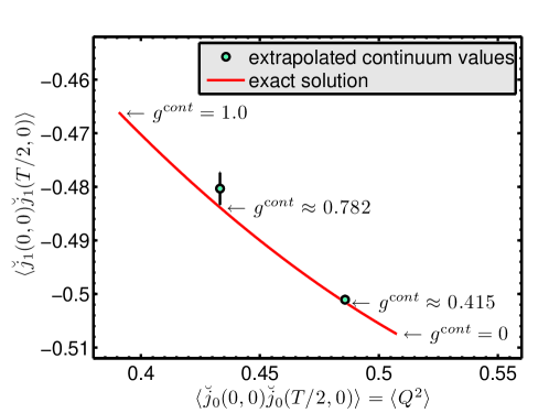
Figure 1: Exact universal relation between current correlations in the massless Thirring model ($N=2$).

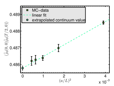
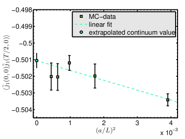
Figure 2: Continuum extrapolations producing the lower point in Fig. 1.

We have extended the well known exact continuum solution of the Thirring model to our finite geometry and plan to report on this elsewhere [7]. This allows to predict many correlation functions. As usual, correlations of the U(1) current

$$\breve{j}_{\mu}(x_{0},p_{1})=\int_{0}^{L}dx_{1}\,\mathrm{e}^{-ip_{1}x_{1}}\bar{\psi}\gamma_{\mu}\psi(x)$$ (16)

are particularly easy to obtain, where we use one Dirac field here at $N=2$. In this case the symmetry (2) gets automatically promoted to an axial U(1). Correlations depend on the continuum coupling $g^{\rm cont}$. By varying it we produce the curve in Fig. 1. Note that the quantity on the $x$-axis is the thermal expectation value of the squared total charge on our ring.

In the lattice transcription we employ the exact Noether U(1) current that does not renormalize. We take the continuum limit by extrapolating from $L/a=16\dots 48$ for values $g=0.4$ and $0.7$ of the bare lattice coupling. The mass is tuned to $m_{c}$ defined by (6) on each lattice. The extrapolations for $g=0.4$, leading to the lower point in Fig. 1 are shown in Fig. 2. The other point is similar but with larger errors.

5 Gross Neveu model ($N=8$)

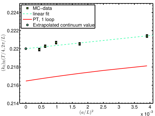
Figure 3: Continuum limit of a Gross-Neveu correlation at $N=8$.

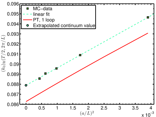
Figure 4: As in Fig. 3, but for a different time separation.

Here the coupling renormalizes similarly to QCD. We now adjust the coupling (8) to the value $g_{R}=0.38$ and take the continuum limit as discussed before. Our universal observable in this case is

$$(k_{\mu})_{R}(x_{0},p_{1})=-\frac{1}{NZ_{\xi}}a\sum_{x_{1}}\mathrm{e}^{-ip_{1}x_{1}}\left\langle\xi^{\top}(0)\mathcal{C}\gamma_{\mu}\xi(x)\right\rangle$$ (17)

for scalable $x_{0}$ values and admissible $p_{1}$. Two examples are shown Fig. 3 and Fig. 4.

6 Remarks on staggered fermions

For naive Majorana lattice fermions, i. e. leaving out the ($\propto a$) part in (3), we find the usual taste multiplicity $2^{D}$ in $D$ dimensions (each momentum component around 0 or $\pi/a$). If one now tries to ‘spin-diagonalize’ by transforming $\xi$ one can only achieve a reduction factor $2^{D/2-1}$ in contrast to $2^{D/2}$ for Dirac fermions when $\psi,\bar{\psi}$ are changed independently. The reason is that $\mathcal{C}$ can only be reduced to $2\times 2$ blocks in the Majorana case but not diagonalized. Since the Majorana form is natural for GN we simply deal here with naive fermions and 4 tastes (on top of $N$ flavors).

The 4-fermion interaction term naively would read in 2-momentum space

$$\frac{1}{(TL)^{4}}\sum_{p_{1},\ldots,p_{4}}\delta^{2}\left(\sum p_{i}\right)\underbrace{\tilde{\xi}_{i}^{\top}(p_{1})\mathcal{C}\tilde{\xi}_{i}(p_{2})}_{\rm taste-mixing}\tilde{\xi}_{j}^{\top}(p_{3})\mathcal{C}\tilde{\xi}_{j}(p_{4}).$$

As indicated, there would be contributions with for instance $p_{1}$ and $p_{2}$ in different corners of the Brillouin zone which mix tastes in the bilinears that are flavor-scalar. This problem was already solved in an early effort to simulate the model [8]. An additional factor $\prod_{\mu}\cos(a(p_{1}+p_{2})_{\mu}/2)\cos(a(p_{3}+p_{4})_{\mu}/2)$ under the sum is expected to enforce taste symmetry in the continuum limit. In position space this corresponds to distributing the interaction term over a plaquette. In this form one then naively expects an additional taste symmetry in the continuum limit which may reproduce results with exact flavor symmetry in the Wilson formulation.
Acknowledgement: We would like to thank Björn Leder and Peter Weisz for critically reading this manuscript.

References

- [1] S. Sharpe, talk at this conference.
- [2] D. J. Gross and A. Neveu, Phys. Rev. D 10, 3235 (1974).
- [3] T. Korzec, F. Knechtli, U. Wolff and B. Leder, PoS LAT2005, 267 (2006) [arXiv:hep-lat/0509132].
- [4] S. Aoki and K. Higashijima, Prog. Theor. Phys. 76, 521 (1986).
- [5] R. Kenna and J. C. Sexton, Phys. Rev. D 65, 014507 (2002) [arXiv:hep-lat/0103014].
- [6] B. Leder and T. Korzec, PoS LAT2005, 266 (2006) [arXiv:hep-lat/0509144].
- [7] T. Korzec and U. Wolff, in preparation
- [8] Y. Cohen, S. Elitzur and E. Rabinovici, Nucl. Phys. B 220, 102 (1983).