DESY 06-163 LTH-716 RM3-TH/06-14 SFB/CPP-06-43 WUB 06-04
Iterative methods for overlap and twisted mass fermions

Abstract

We present a comparison of a number of iterative solvers of linear systems of equations for obtaining the fermion propagator in lattice QCD. In particular, we consider chirally invariant overlap and chirally improved Wilson (maximally) twisted mass fermions. The comparison of both formulations of lattice QCD is performed at four fixed values of the pion mass between 230MeV and 720MeV. For overlap fermions we address adaptive precision and low mode preconditioning while for twisted mass fermions we discuss even/odd preconditioning. Taking the best available algorithms in each case we find that calculations with the overlap operator are by a factor of 30-120 more expensive than with the twisted mass operator.

1 Introduction

Certainly, the available computer power has advanced impressively over the last years. Nevertheless, for obtaining high precision simulation results in lattice QCD, as our target application in this paper, it remains essential to improve –on the one hand– the algorithms employed for lattice simulations and –on the other hand– to find better formulations of lattice fermions. Two very promising candidates for improved versions of lattice fermions are chirally invariant [1] overlap fermions [2, 3] and chirally improved Wilson twisted mass (TM) fermions [4] at maximal twist. Both have the potential to overcome some basic difficulties of lattice QCD, most notably they make simulations at values of the pseudo scalar mass close to the experimentally observed pion mass of $140$MeV possible. For a comparison of physical results obtained with the two mentioned operators in the quenched approximation see Ref. [5].

The reason for these difficulties is that one has to solve a huge set of linear equations over and over again. Although, due to the only nearest neighbour interaction of the underlying Wilson-Dirac operator, sparse matrix methods can be employed, the computational cost can get extremely large, see, e.g. the discussions in Refs. [6, 7, 8].

The focus of this work is to compare different iterative linear solvers for sparse matrices as needed for computing the quark propagator for valence quarks or for the computation of the fermionic ”force” in dynamical simulations. It has to be remarked that the exact behaviour of sparse matrix methods is highly problem specific and can depend strongly on the underlying matrix involved. It is hence crucial to compare the optimal method for a given kind of lattice fermion. In our case, we will consider overlap fermions and Wilson twisted mass fermions at maximal twist. We will explore a number of sparse matrix methods for the solution of the linear system defined by the corresponding lattice Dirac operator. Although we have tried to be rather comprehensive, it is clear that such a work cannot be exhaustive. The set of possible linear solvers is too large to be able to cover all of them, see e.g. [9] and different solvers may be better for different situations. For example, if we are only interested in computing fermion propagators, the question is, whether we want to have a multiple mass solver [10]. Or, with respect of dynamical simulations, we need the square of the lattice Dirac operator and not the operator itself which can lead to very different behaviour of the algorithm employed. In addition, each of the basic algorithms can be combined with certain improvement techniques which again influence the algorithm behaviour substantially.

In principle, it is also desirable to study the performance behaviour of the algorithms as a function of the pseudo scalar mass, the lattice volume and the lattice spacing. Again, in this work, due to the very costly simulations such a study would require, we have to restrict ourselves to an only limited set of parameters. In particular, we will consider two physical volumes and four values of the pseudo scalar mass (matched between both formulations of lattice QCD). Finally, we will only take one value of the lattice spacing for our study.

As an outcome of this work, we will find that the computational cost of particular algorithms and variants thereof can vary substantially for different situations. This gives rise to the conclusion that it can be very profitable to test the –at least most promising– algorithms for the particular problem one is interested in. It is one of our main conclusions that easily a factor of two or larger can be gained when the algorithm is adopted to the particular problem under consideration.

Parts of the results presented in this paper were already published in Ref. [11] and for related work concerning the overlap operator see Refs. [12, 13, 14].

The outline of the paper is as follows. In section 2 we introduce the Dirac operators that are considered in this study. Section 3 discusses the iterative linear solver algorithms and special variants thereof, like multiple mass solvers and, for the overlap operator, adaptive precision solvers and solvers in a given chiral sector. In section 4 we present various preconditioning techniques like even/odd preconditioning for the TM operator and low mode preconditioning for the overlap operator. In section 5 we present and discuss our results and in section 6 we finish with conclusions and an outlook. Appendix A deals with the computation of eigenvalues and eigenvectors which is important for an efficient implementation of the overlap operator, for its low mode preconditioning and for the computation of its index. Appendix B finally reformulates the TM operator so that multiple mass solvers become applicable.

2 Lattice Dirac operators

We consider QCD on a four-dimensional hyper-cubic lattice in Euclidean space-time. The fermionic fields $\psi$ live on the sites $x$ of the lattice while the SU(3) gauge fields of the theory are represented by group-valued link variables $U_{\mu}(x),\mu=1,\ldots,4$. The gauge covariant backward and forward difference operators are given by

$$\begin{split}(\nabla_{\mu}\psi)(x)&=U_{\mu}(x)\psi(x+\hat{\mu})-\psi(x),\\ (\nabla^{*}_{\mu}\psi)(x)&=\psi(x)-U^{\dagger}_{\mu}(x-\hat{\mu})\psi(x-\hat{\mu}),\end{split}$$ (1)

and the standard Wilson-Dirac operator with bare quark mass $m_{0}$ can be written as

$$D_{\text{W}}(m_{0})=\sum_{\mu=1}^{4}\frac{1}{2}\{\gamma_{\mu}(\nabla_{\mu}+\nabla^{*}_{\mu})-\nabla^{*}_{\mu}\nabla_{\mu}\}+m_{0}.$$ (2)

The twisted mass lattice Dirac operator for a $SU_{f}(2)$ flavour doublet of mass degenerate quarks has the form [15, 16]

$$D_{\text{tm}}(\mu_{\mathrm{tm}})=D_{\text{W}}(m_{0})+i\mu_{\mathrm{tm}}\gamma_{5}\tau_{3}\,,$$ (3)

where $D_{\text{W}}$ is the Wilson-Dirac operator with bare quark mass $m_{0}$ as defined above, $\mu_{\mathrm{tm}}$ the twisted quark mass and $\tau_{3}$ the third Pauli matrix acting in flavour space. Since it was shown in Ref. [4] (for a test in practise see Refs. [17, 18]) that physical observables are automatically $O(a)$ improved if $m_{0}$ is tuned to its critical value, we are only interested in this special case.

The second operator we consider, the massive overlap operator, is defined as [2, 3]

$$D(\mu_{\mathrm{ov}})=\Big{(}1-\frac{\mu_{\mathrm{ov}}}{2M}\Big{)}D+\mu_{\mathrm{ov}}\,,$$ (4)

where

$$D=M\Big{(}1+\gamma_{5}\operatorname{sign}\left[Q(-M)\right]\Big{)}\,$$ (5)

is the massless overlap operator, $Q(-M)=\gamma_{5}D_{\text{W}}(-M)$ with $M$ chosen to be $M=1.6$ in this work and $\mu_{\mathrm{ov}}$ again the bare quark mass. The matrix $\operatorname{sign}$-function in Eq.(5) is calculated by some approximation that covers the whole spectrum of $Q(-M)$. To make this feasible we determine $K$ eigenmodes of $Q(-M)$ closest to the origin, project them out from the $\operatorname{sign}$-function and calculate their contribution analytically while the rest of the spectrum is covered by an approximation employing Chebysheff polynomials. Denoting by $\psi_{k}$ the eigenvectors of $Q$ with corresponding eigenvalue $\lambda_{k}$, i.e. $Q\psi_{k}=\lambda_{k}\psi_{k}$, we have

$$\begin{split}\operatorname{sign}\left[Q(-M)\right]=&\sum_{k=1}^{K}\operatorname{sign}(\lambda_{k})P_{k}+\\ &\left(1-\sum_{k=1}^{K}P_{k}\right)Q\cdot T_{N}\left[Q^{2}\right]\left(1-\sum_{k=1}^{K}P_{k}\right)\,,\\ \end{split}$$ (6)

where $P_{k}=\psi_{k}\psi_{k}^{\dagger}$ are projectors onto the eigenmode subspaces and $T_{N}\left[Q^{2}\right]$ denotes the $N$-th order Chebysheff polynomial approximation to $1/\sqrt{(}Q^{2})$ on the orthogonal subspace. The calculation of the eigenmodes is discussed in appendix A.

3 Iterative linear solver algorithms

Let us now turn to the iterative linear solver algorithms that we consider in our investigation. Table 1 lists the various algorithms and marks with ’x’ which of them are used with the overlap and the TM operator, respectively. For the convenience of the reader we also compile in table 1 for each algorithm the number of operator applications, i.e. matrix-vector (MV) multiplications, together with the corresponding number of scalar products (SP) and linear algebra instructions $Z=\alpha X+Y$ (ZAXPY) per iteration. Moreover, in the last column we also note which of the algorithms possess the capability of using multiple masses (MM).

$\Bigl{.}\Bigr{.}$Algorithm	Overlap	TM	MV	SP	ZAXPY	MM
CGNE [9]	x	x	2	2	3	yes
CGS [9]	x	x	2	2	7	yes
BiCGstab [9]	x	x	2	4	6	yes
GMRES(m) [9]	x	x	1	$m/2+1$	$m/2+1$	no
MR [9]	x	x	1	2	2	yes
CGNEχ	x		1	2	3	yes
SUMR [19]	x		1	6	1	yes

Table 1: Linear solver algorithms for the overlap and twisted mass (TM) operator. Also given are the number of matrix vector (MV) multiplications, scalar products (SP) and $z=\alpha x+y$ (ZAXPY) linear algebra operations per iteration. We also indicate, whether the algorithm can be used to solve for multiple masses (MM).

With the exception of the MR algorithm all algorithms are Krylov subspace methods, i.e. they construct the solution of the linear system $A\psi=\eta$ as a linear combination of vectors in the Krylov subspace

$$\mathcal{K}_{i}=\text{span}(v,Av,\ldots,A^{i-1}v)\,,$$

where $v=r_{0}=\eta-A\psi_{0}$ is the initial residual. In contrast the MR algorithm is a one-dimensional projection process [9], i.e. each iteration step is completely independent of the previous one. For a detailed description and discussion of the basic algorithms we refer to [9], whereas we will discuss some special versions in the following subsections. Note that we adopted the names of the algorithms from Ref. [20] where possible.

The SUMR algorithm was introduced in Ref. [19] and first used for lattice QCD in Ref. [12]. It makes use of the unitarity property of the massless overlap operator and was shown to perform rather well when compared to other standard iterative solvers [12].

In the case of TM fermions it is sometimes useful to consider the linear system $\gamma_{5}A\psi=\gamma_{5}\eta$ instead of $A\psi=\eta$. The reason for the importance of this change will be discussed later. We will add a $\gamma_{5}$ to the solver name in case the changed system is solved, like for instance CGS$\gamma_{5}$.

3.1 Multiple mass solvers

In propagator calculations for QCD applications it is often necessary to compute solutions of the system

$$(A+\sigma)\psi=\eta$$ (7)

for several values of a scalar shift $\sigma$ - usually the mass. It has been realised some time ago [10, 21, 22, 23] that the solutions of the shifted systems can be obtained at largely the cost of only solving the system with the smallest (positive) shift. For the Krylov space solvers this is achieved by realising that the Krylov spaces of the shifted systems are essentially the same. In table 1 we note in the last column which of the algorithms can be implemented with multiple masses. Multiple mass (MM) versions for BiCGstab and CG can be found in [22]. In principle there exists also a MM version for the GMRES algorithm, but since in practise the GMRES has to be restarted after $m$ iteration steps it does not carry over to the case of GMRES($m$). For the SUMR algorithm we note that the MM version is trivial, since the shift of the unitary matrix enters in the algorithm not via the iterated vectors but instead only through scalar coefficients directly into the solution vector.

Finally we wish to emphasise that also the CGNE algorithm is capable of using multiple masses in special situations. This remark is non-trivial since in general $(A^{\dagger}+\sigma)(A+\sigma)$ appearing in the normal equation is not of the form $A^{\prime\dagger}A^{\prime}+\sigma^{\prime}$. However, it turns out that for the overlap operator and the twisted mass operator a MM is possible. For the overlap operator one can make use of the Ginsparg-Wilson relation in order to bring the shifted normal equation operator into the desired form [24]. For the Wilson twisted mass fermion operator we provide in Appendix B the details of the MM implementation for CGNE.

3.2 Chiral CGNE for the overlap operator

Due to the fact that the overlap operator obeys the Ginsparg-Wilson relation it is easy to show that $D^{\dagger}D$ commutes with $\gamma_{5}$. As a consequence the solution to the normal equation $D^{\dagger}D\psi=\eta$ can be found in a given chiral sector as long as the original source vector $\eta$ is chiral. (This is for example the case if one works with point sources in a chiral basis.)

When applying the CGNE algorithm to the overlap operator one can then make use of this fact by noting the relation

$$P_{\pm}D(\mu_{\text{ov}})^{\dagger}D(\mu_{\text{ov}})P_{\pm}=2MP_{\pm}D(\mu_{\text{ov}}^{2}/(2M))P_{\pm}\,,$$ (8)

where $P_{\pm}=1/2(1\pm\gamma_{5})$ are the chiral projectors. Thus in each iteration the operator is only applied once instead of twice, but with a modified mass parameter. This immediately saves a factor of two in the number of matrix-vector (MV) applications with respect to the general case. In table 1 and in the following we denote this algorithm by CGNE_χ.

3.3 Adaptive precision solvers for the overlap operator

It is well known that the computational bottleneck for the solvers employing the overlap operator is the computation of the approximation of the sign-function $\text{sign}(Q)$. Since each application of the overlap operator during the iterative solver process requires yet another iterative procedure to approximate $\operatorname{sign}(Q)$, we are led to a two-level nested iterative procedure where the cost for the calculation of the sign-function enters multiplicatively in the total cost. So any optimised algorithm will not only aim at minimising the number of outer iterations, i.e. the number of overlap operator applications, but it will also try to reduce the number of inner iterations, i.e. the order of the – in our case polynomial – approximation.

While the problem of minimising the number of outer iterations depends on a delicate interplay between the algorithm and the operator under consideration and comprises one of the main foci of the present investigation, the problem to reduce the number of inner iterations can be achieved rather directly in two different ways. Firstly, as discussed in section 2, we project out the lowest 20 or 40 eigenvectors of the Wilson-Dirac operator depending on the extent of the lattice (cf. section 5.1). In this way we achieve that our approximations use (Chebysheff) polynomials typically of the order $O(200-300)$ for the simulation parameters we have employed for this study.

Secondly, it is then also clear that one can speed up the calculations by large factors if it is possible to reduce the accuracy of the approximation. In realising this, the basic idea is to adapt the degree of the polynomial during the solver iteration to achieve only that precision as actually needed in the present iteration step. We have implemented the adaptive precision for a selection of the algorithms that seemed most promising in our first tests and in the following we denote these algorithms by the subscript ${}_{\text{ap}}$ for adaptive precision. Usually not more than two lines of additional code are required to implement the adaptive precision versions of the algorithms. Obviously the details of how exactly one needs to adapt the precision of the polynomial depends on the details of the algorithm itself and might also influence the possibility to do multi mass inversions.

We use two generic approaches which we illustrate in the following by means of the adaptive precision versions of the MR and the CGNE algorithms, respectively. In the case of the MR we follow a strategy that is similar to restarting: through the complete course of the iterative procedure we use a low order polynomial approximation of a degree $O(10)$ for the $\operatorname{sign}$ function. Only every $m$ iteration steps we correct for the errors by computing the true residuum to full precision, which corresponds essentially to a restart of the algorithm. We denote this algorithm with MR${}_{\mathrm{ap}}(m)$. We remark that with this approach the MM capability of the MR algorithm is lost.

The MR${}_{\mathrm{ap}}(m)$ is outlined with pseudo-code in algorithm 1, where we denote the low order approximation of the overlap operator with $A_{\mathrm{ap}}$ while the full precision operator is denoted with $A$.

Algorithm 1 MR${}_{\mathrm{ap}}(A,A_{\mathrm{ap}},b,x,m,\epsilon)$ algorithm

1:  $i=0$

2:  $p=Ax$

3:  $r=b-p$

4:  repeat

5:     $i=i+1$

6:     // Use $A_{\mathrm{ap}}$ with fixed low order polynomial

7:     $\tilde{r}=A_{\mathrm{ap}}r$

8:     $\alpha=(\tilde{r},r)/(\tilde{r},\tilde{r})$

9:     $x=x+\alpha r$

10:     if $i\mod m=0$ then

11:        // Correct with full $A$

12:        $p=Ax$

13:     else

14:        $p=p+\alpha\tilde{r}$

15:     end if

16:     $r=b-p$

17:  until $\|r\|<\epsilon$

The same approach as used for the MR${}_{\mathrm{ap}}(m)$ algorithm can easily be carried forward to the GMRES${}_{\mathrm{ap}}(m)$ algorithm. Since the GMRES$(m)$ is restarted every $m$ iterations, we use only every $m$-th iteration the full approximation to the $\operatorname{sign}$ function while all other applications of the overlap operator are performed with an approximation of degree $O(10)$.

In case of the CGNE_ap our strategy is different: here we simply calculate contributions to the $\operatorname{sign}$-function approximation up to the point where they are smaller than $\epsilon_{\mathrm{ap}}=10^{-2}\epsilon$, where $\epsilon$ is the desired final residual, i.e. we neglect all corrections that are much smaller than the final residual. This requires the full polynomial only at the beginning of the CG-search while towards the end of the search we use polynomials with a degree $O(10)$. In order to implement this idea we use a forward recursion scheme for the application of the Chebysheff polynomial as detailed in algorithm 2.

Algorithm 2 Compute $r=\sum_{j=0}^{n-1}c_{j}T_{j}(Q^{2})\,v$ to precision $\epsilon_{\mathrm{ap}}$

0:  vector $v$ and Chebysheff coefficients $c_{j}$

1:  $d_{0}=T_{0}(Q^{2})\,v=v$

2:  $d_{1}=T_{1}(Q^{2})\,v=2\,Q^{2}\,v-v$

3:  $r=c_{1}d_{1}+1/2c_{0}d_{0}$

4:  for j=2,…,n-1 do

5:     $d_{j}=T_{j}(Q^{2})\,v=2\,Q^{2}\,d_{j-1}-d_{j-2}$

6:     $r=r+c_{j}d_{j}$

7:     if $\|d_{j}\|<\epsilon_{\mathrm{ap}}$ then

8:        return $r$

9:     end if

10:  end for

11:  return $r$

It is important to note here that with this approach for the CGNE${}_{\text{ap}}$ the MM capability is preserved (in contrast to an approach proposed in Ref. [25] similar to the MR${}_{\text{ap}}(m)$ approach described above where the MM capability is lost). The strategy for the SUMR${}_{\text{ap}}$ is analogous to the one for the CGNE${}_{\text{ap}}$, where again the MM capability is preserved.

4 Preconditioning techniques

4.1 Even/odd preconditioning for the TM operator

Even/odd preconditioning for the Wilson TM operator has already been described in [26] and we review it here for completeness only. Let us start with the hermitian two flavour Wilson TM operator in the hopping parameter representation ($\kappa=(2m_{0}+8)^{-1}$)

$$Q\equiv\gamma_{5}D=\begin{pmatrix}Q^{+}&\\ \ &Q^{-}\\ \end{pmatrix}\,,$$ (9)

where the sub-matrices $Q^{\pm}$ can be factorised with $\tilde{\mu}=2\kappa\mu$ as follows:

$$\begin{split}Q^{\pm}&=\gamma_{5}\begin{pmatrix}1\pm i\tilde{\mu}\gamma_{5}&D_{eo}\\ D_{oe}&1\pm i\tilde{\mu}\gamma_{5}\\ \end{pmatrix}=\gamma_{5}\begin{pmatrix}D_{ee}^{\pm}&D_{eo}\\ D_{oe}&D_{oo}^{\pm}\\ \end{pmatrix}\\ &=\begin{pmatrix}\gamma_{5}D_{ee}^{\pm}&0\\ \gamma_{5}D_{oe}&1\\ \end{pmatrix}\begin{pmatrix}1&(D_{ee}^{\pm})^{-1}D_{eo}\\ 0&\gamma_{5}(D_{oo}^{\pm}-D_{oe}(D_{ee}^{\pm})^{-1}D_{eo})\\ \end{pmatrix}\,.\end{split}$$ (10)

Note that $(D_{ee}^{\pm})$ is trivial to invert:

$$(1\pm i\tilde{\mu}\gamma_{5})^{-1}=\frac{1\mp i\tilde{\mu}\gamma_{5}}{1+\tilde{\mu}^{2}}.$$ (11)

Due to the factorisation (10) the full fermion matrix can be inverted by inverting the two matrices appearing in the factorisation

$$\begin{pmatrix}D_{ee}^{\pm}&D_{eo}\\ D_{oe}&D_{oo}^{\pm}\\ \end{pmatrix}^{-1}=\begin{pmatrix}1&(D_{ee}^{\pm})^{-1}D_{eo}\\ 0&(D_{oo}^{\pm}-D_{oe}(D_{ee}^{\pm})^{-1}D_{eo})\\ \end{pmatrix}^{-1}\begin{pmatrix}D_{ee}^{\pm}&0\\ D_{oe}&1\\ \end{pmatrix}^{-1}\,.$$

and the two factors can be simplified as follows:

$$\begin{pmatrix}D_{ee}^{\pm}&0\\ D_{oe}&1\\ \end{pmatrix}^{-1}=\begin{pmatrix}(D_{ee}^{\pm})^{-1}&0\\ -D_{oe}(D_{ee}^{\pm})^{-1}&1\\ \end{pmatrix}$$

and

$$\begin{split}&\begin{pmatrix}1&(D_{ee}^{\pm})^{-1}D_{eo}\\ 0&(D_{oo}^{\pm}-D_{oe}(D_{ee}^{\pm})^{-1}D_{eo})\\ \end{pmatrix}^{-1}\\ =&\begin{pmatrix}1&-(D_{ee}^{\pm})^{-1}D_{eo}(D_{oo}^{\pm}-D_{oe}(D_{ee}^{\pm})^{-1}D_{eo})^{-1}\\ 0&(D_{oo}^{\pm}-D_{oe}(D_{ee}^{\pm})^{-1}D_{eo})^{-1}\\ \end{pmatrix}\,.\end{split}$$

The complete inversion is now performed in two separate steps: First we compute for a given source field $\phi=(\phi_{e},\phi_{o})$ an intermediate result $\varphi=(\varphi_{e},\varphi_{o})$ by:

$$\begin{pmatrix}\varphi_{e}\\ \varphi_{o}\\ \end{pmatrix}=\begin{pmatrix}D_{ee}^{\pm}&0\\ D_{oe}&1\\ \end{pmatrix}^{-1}\begin{pmatrix}\phi_{e}\\ \phi_{o}\\ \end{pmatrix}=\begin{pmatrix}(D_{ee}^{\pm})^{-1}\phi_{e}\\ -D_{oe}(D_{ee}^{\pm})^{-1}\phi_{e}+\phi_{o}\\ \end{pmatrix}\,.$$

This step requires only the application of $D_{oe}$ and $(D_{ee}^{\pm})^{-1}$, the latter of which is given by Eq.(11). The final solution $\psi=(\psi_{e},\psi_{o})$ can then be computed with

$$\begin{pmatrix}\psi_{e}\\ \psi_{o}\\ \end{pmatrix}=\begin{pmatrix}1&(D_{ee}^{\pm})^{-1}D_{eo}\\ 0&(D_{oo}^{\pm}-D_{oe}(D_{ee}^{\pm})^{-1}D_{eo})\\ \end{pmatrix}^{-1}\begin{pmatrix}\varphi_{e}\\ \varphi_{o}\\ \end{pmatrix}=\begin{pmatrix}\varphi_{e}-(D_{ee}^{\pm})^{-1}D_{eo}\psi_{o}\\ \psi_{o}\\ \end{pmatrix}\,,$$

where we defined

$$\psi_{o}=(D_{oo}^{\pm}-D_{oe}(D_{ee}^{\pm})^{-1}D_{eo})^{-1}\varphi_{o}\,=\hat{D}^{-1}\varphi_{o}\,.$$ (12)

Therefore the only inversion that has to be performed numerically is the one to generate $\psi_{o}$ from $\varphi_{o}$ and this inversion involves only $\hat{D}$ that is better conditioned than the original fermion operator.

A similar approach is to invert in Eq.(12) instead of $\hat{D}$ the following operator:

$$\hat{D}_{s}=1-(D_{oo}^{\pm})^{-1}D_{oe}(D_{ee}^{\pm})^{-1}D_{eo}\,,$$

on the source $(D_{oo}^{\pm})^{-1}\varphi_{o}$. As noticed already in Ref. [27] for the case of non-perturbatively improved Wilson fermions this more symmetrical treatment results in a slightly better condition number leading to $20\%$ less iterations in the solvers.

4.2 Low mode preconditioning for the overlap operator

Low mode preconditioning (LMP) for the overlap operator has already been described in Ref. [25] using the CG algorithm on the normal equations. In case of the CG the operator $D^{\dagger}D$ to be inverted is hermitian, and hence normal, and the low mode preconditioning is as described in Ref. [25].

The application of this technique to algorithms like GMRES or MR (which involve $D$ instead of $D^{\dagger}D$) is not completely straightforward. Although the overlap operator itself is formally normal, in practise it is not due to the errors introduced by the finite approximation of the $\operatorname{sign}$-function. As a consequence one has to distinguish between left and right eigenvectors of $D$ leading to some additional complications which we are now going to discuss.

Consider the linear equation $A\psi=\eta$. The vector space on which the linear operator $A$ acts can be split into two (bi-)orthogonal pieces using the (bi-)orthogonal projectors

$$P=\sum_{k}r_{k}l_{k}^{\dagger},\quad P_{\perp}=1-P.$$ (13)

Here we assume that the $r_{k}^{\prime}s$ and $l_{k}^{\prime}s$ are approximate right and left eigenvectors (Ritz vectors), respectively, of the operator $A$ which form a bi-orthogonal basis, i.e. $l_{i}^{\dagger}r_{j}=\delta_{ij}$. One can write

$$Ar_{k} = \alpha_{k}r_{k}+g_{k}^{(r)}\,,$$ (14)

$$A^{\dagger}l_{k} = \bar{\alpha}_{k}l_{k}+g_{k}^{(l)}\,,$$ (15)

where $l_{i}^{\dagger}g_{k}^{(r)}=r_{i}^{\dagger}g_{k}^{(l)}=0$. Indeed, one finds

$$PAr_{k}=\alpha_{k}r_{k}$$ (16)

and

$$P_{\perp}Ar_{k}=g_{k}^{(r)}.$$ (17)

The operator $A$ then takes the following block form

$$A=\left(\begin{array}[]{cc}PAP&PAP_{\perp}\\ P_{\perp}AP&P_{\perp}AP_{\perp}\end{array}\right)$$ (18)

and the linear equation reads

$$\left(\begin{array}[]{cc}PAP&PAP_{\perp}\\ P_{\perp}AP&P_{\perp}AP_{\perp}\end{array}\right)\left(\begin{array}[]{c}P\psi\\ P_{\perp}\psi\end{array}\right)=\left(\begin{array}[]{c}P\eta\\ P_{\perp}\eta\end{array}\right).$$ (19)

To solve this equation we can perform a LU decomposition of $A$

$$A=\left(\begin{array}[]{cc}1&0\\ P_{\perp}AP(PAP)^{-1}&1\end{array}\right)\left(\begin{array}[]{cc}PAP&PAP_{\perp}\\ 0&S\end{array}\right)\equiv L\cdot U\,,$$ (20)

where $S=P_{\perp}AP_{\perp}-P_{\perp}AP(PAP)^{-1}PAP_{\perp}$ is the Schur complement of $A$. The lower triangular matrix $L$ can be inverted and applied to the right hand side,

$$L^{-1}\eta=\left(\begin{array}[]{c}P\eta\\ -P_{\perp}AP(PAP)^{-1}P\eta+P_{\perp}\eta\end{array}\right),$$ (21)

and the linear system reduces to solving $U(P\psi,P_{\perp}\psi)^{T}=L^{-1}\eta$. Written out explicitly we obtain the second component $P_{\perp}\psi$ from solving the equation

$$P_{\perp}(A-AP(PAP)^{-1}PA)P_{\perp}\psi=P_{\perp}\eta-P_{\perp}AP(PAP)^{-1}P\eta$$ (22)

and the first component $P\psi$ from the solution of

$$PAP\cdot P\psi=P\eta-PAP_{\perp}\psi.$$ (23)

In detail the whole procedure to solve $A\psi=\eta$ using low mode preconditioning involves the following steps:

1. prepare (precondition) the source according to the r.h.s. of Eq.(22), i.e.

   $$\eta^{\prime}=P_{\perp}\left(1-\sum_{i}g_{i}^{(r)}\frac{1}{\alpha_{i}}l_{i}^{\dagger}\right)\eta\,,$$ (24)

   where we have used $P_{\perp}r_{i}=0$.

2. solve the low mode preconditioned system $A_{\text{lmp}}P_{\perp}\psi=\eta^{\prime}$ for $P_{\perp}\psi$ where $A_{\text{lmp}}$ is the preconditioned operator acting in the subspace orthogonal to the low modes, i.e. the operator on the l.h.s. of Eq.(22). To be specific the application of the preconditioned operator is given by

   $$P_{\perp}\left[A-AP(PAP)^{-1}PA)\right]P_{\perp}\psi=\\ P_{\perp}\left[A-\sum_{i,j,k}\left(\alpha_{i}r_{i}+g_{i}^{(r)}\right)l_{i}^{\dagger}r_{j}\frac{1}{\alpha_{j}}l_{j}^{\dagger}r_{k}\left(l_{k}^{\dagger}\alpha_{k}+g_{k}^{(l)}{}^{\dagger}\right)\right]P_{\perp}\psi\\ =P_{\perp}\left[A-\sum_{i}g_{i}^{(r)}\frac{1}{\alpha_{i}}g_{i}^{(l)}{}^{\dagger}\right]P_{\perp}\psi\,,$$ (25)

   where we have used $P_{\perp}r_{i}=l_{k}^{\dagger}P_{\perp}=0$.

3. add in the part of the solution from the subspace spanned by the low modes, i.e. $P\psi$. This part is essentially the contribution from the low modes and it is explicitly given by

   $$P\psi=\sum_{i}r_{i}\frac{1}{\alpha_{i}}l_{i}^{\dagger}(\eta-AP_{\perp}\psi).$$ (26)

Let us mention for completeness that there are further related preconditioning techniques available which do not involve the analytic correction step in Eq.(26). The Ritz vectors can be used directly in any right or left preconditioned version of a given solver like for instance in the FGMRES algorithm [20]. Moreover, the computation of the Ritz pairs and the iterative solution can be combined in so called iterative solvers with deflated eigenvalues, see for instance the GMRES versions discussed in Refs.[9, 28, 29].

5 Results

In this section we are going to present our numerical results. We organise the discussion in the following way: we first look at the two operators we have used separately. For each of them we examine the mass and volume dependence of the numerical effort without and with improvements for the solvers and preconditioning techniques switched on. For the overlap operator we then test in addition the low mode preconditioning approach in the $\epsilon$–regime. After discussing them separately we will then compare the two operators by means of the best solver.

The algorithms are compared for each operator using the following criteria:

1. The total iteration number:
   The number of iterations to reach convergence is a quantity which is independent of the detailed implementation of the Dirac operator as well as of the machine architecture, and therefore it provides a fair measure for comparison.

2. The total number of applications of $Q$:
   In particular in case of the adaptive precision algorithms of the overlap operator, it turns out that the cost for one iteration depends strongly on the algorithm details, so a fairer mean for comparison in that case is the total number of applications of the Wilson-Dirac operator, i.e. the number of $Q$ applications. Again this yields a comparative measure independent of the architecture and the details of the operator implementation, but on the other hand one should keep in mind that these first two criteria neglect the cost stemming from scalar products and ZAXPY operations. In particular this concerns the GMRES algorithm that needs significantly more of these operations than the other algorithms. It also concerns the adaptive precision algorithms for the overlap operator for reasons explained below.

3. The total execution time in seconds:
   Finally, in order to study the relative cost factor between the inversion of the TM and the overlap operator we measure for each operator and algorithm the absolute timings on a specific machine, in our case on one node of the Jülich Multiprocessor (JUMP) IBM p690 Regatta using 32 processors. Obviously, these results will depend on the specific details of the machine architecture and the particular operator and linear algebra implementation, and hence will have no absolute validity. Nevertheless, it is interesting to strive to such a comparison simply to obtain at least a feeling for the order of magnitude of the relative cost.

5.1 Set-up

Our set-up consists of two quenched ensembles of 20 configurations with volumes $V=12^{4}$ and $16^{4}$ generated with the Wilson gauge action at $\beta=5.85$ corresponding to a lattice spacing of $a\sim 0.125$ fm ($r_{0}=0.5$ fm).

The bare quark masses for the overlap operator and the twisted mass operator are chosen such that the corresponding pion mass values are matched, cf. table 2. Note that for the low mode preconditioning of the overlap operator we consider an additional small mass which should bring the system into the $\varepsilon$–regime.

$\Bigl{.}\Bigr{.}m_{\pi}$[MeV]	$\mu_{\textrm{ov}}$	$\mu_{\textrm{tm}}$
720	0.10	0.042
555	0.06	0.025
390	0.03	0.0125
230	0.01	0.004
$\epsilon$-regime	0.005	–

Table 2: Bare quark masses for the overlap and the twisted mass operator matched by the pion mass. The quark mass of $\mu_{\textrm{ov}}=0.005$ corresponds to a simulation point in the $\epsilon$-regime, where the notion of a pion mass becomes meaningless.

We invert the twisted mass (the overlap) operator on one (two) point-like source(s) $\eta$ for each configuration at the four bare quark masses. The required stopping criterion is $\|r\|^{2}=\|Ax-\eta\|^{2}<10^{-14}$, where $r$ is the residual and $x$ the solution vector. We are working in a chiral basis and the two sources for the overlap operator are chosen such that they correspond to sources in two different chiral sectors. This is relevant for the overlap operator only, which might have exact zero modes of the massless operator in one of the two chiral sectors, potentially leading to a quite different convergence behaviour. Furthermore the chiral sources allow to use the chiral version of the CGNE algorithm for the overlap operator as described in section 2. There it is also mentioned that for the overlap operator we project out the lowest 20 and 40 eigenvectors of $Q^{2}$ on the $12^{4}$ and $16^{4}$ lattice, respectively, in order to make the construction of the $\operatorname{sign}$-function feasible.

For both operators we follow the strategy to first consider the not preconditioned algorithms and then to switch on the available preconditionings or improvements. Since for the overlap operator we have a large range of algorithms to test (and the tests are more costly), we perform the first step only at two masses and study the improvements from the preconditioning and the full mass dependence only for a selection of algorithms.

5.2 Twisted mass results

Before presenting results for the un-preconditioned TM Dirac operator, we need to discuss the following point: the number of iterations needed by a certain iterative solver depends in the case of the twisted mass Dirac operator strongly on whether $D_{\mathrm{tm}}$ is inverted on a source $\eta$ or $\gamma_{5}D_{\mathrm{tm}}$ on a source $\gamma_{5}\eta$. This is due to the fact that multiplying with $\gamma_{5}$ significantly changes the eigenvalue distribution of the TM operator. All eigenvalues of $\gamma_{5}D_{\mathrm{tm}}$ lie on a line parallel to the real axis shifted in the imaginary direction by $\mu$, because the pure Wilson-Dirac operator obeys the property $D_{\mathrm{W}}^{\dagger}=\gamma_{5}D_{\mathrm{W}}\gamma_{5}$. To give examples, for the BiCGstab and the GMRES algorithms $\gamma_{5}D_{\mathrm{tm}}$ is advantageous, while the CGS solver works better with $D_{\mathrm{tm}}$ itself.

This result is not surprising: it is well known that for instance the BiCGstab iterative solver is not efficient, or even does not converge, when the eigenvalue spectrum is complex and in exactly such situations the CGS [30] algorithm often performs better. Of course, for the CG solver this question is not relevant, since in that case the operator $D^{\dagger}D$ is used. Let us also mention that neither the MR nor the MR$\gamma_{5}$ iterative solver converged for the twisted mass operator within a reasonable number of iterations.

The results for the un-preconditioned Wilson TM operator are collected in table 3 where we give the average number of operator applications (MV applications) that are required to reach convergence together with the standard deviation. In the case of the TM operator, the number of MV applications is proportional to the number of solver iterations where the proportionality factor can be read off column 4 in table 1.

	$\mu_{\textrm{tm}}=0.042$	$0.025$	$0.0125$	$0.004$
$V=12^{4}$
CGNE	2082(60)	2952(175)	3536(234)	3810(243)
CGS	1251(178)	1661(262)	1920(361)	2251(553)
BiCGstab$\gamma_{5}$	3541(175)	5712(280)	9764(503)	12772(979)
GMRES$\gamma_{5}$	1962(48)	3314(92)	6223(199)	19204(737)
$V=16^{4}$
CGNE	2178(46)	3556(107)	6277(414)	8697(802)
CGS	1336(134)	2029(276)	2614(508)	3420(866)
BiCGstab$\gamma_{5}$	3526(145)	5805(239)	10940(547)	26173(2099)
GMRES$\gamma_{5}$	1945(42)	3287(78)	6168(129)	19106(565)

Table 3: Average number (and standard deviation) of MV applications for reaching convergence of the un-preconditioned Wilson TM operators. Here and in the following tables, averages are always taken over 20 independent pure gauge configurations.

From these data it is clear that the CGS algorithm is the winner for all masses and on both volumes. The CGS algorithm shows a rather weak exponential mass dependence and beats the next best algorithm CGNE by a factor 2.5 at the smallest mass on the large volume as is evident from figure 1 where we plot the logarithm of the absolute timings in units of seconds as a function of the bare quark mass. Since the CGNE shows a similar scaling with the mass as the CGS we do not expect this conclusion to change for smaller masses. Moreover the CGS appears to have a weaker volume dependence than the CGNE, in particular at small masses, so we expect the conclusion to be strengthened as the volume is further increased. A very interesting point to note is that the GMRES$\gamma_{5}$ algorithm shows a perfect scaling with the volume in the sense that the iteration numbers remain constant as the volume is increased.

Figure 1: Average timings for the inversion of the un-preconditioned Wilson TM operator in units of seconds on a logarithmic scale for different bare quark masses. We compare two volumes, a $12^{4}$ (top) and a $16^{4}$ lattice (bottom).

5.2.1 Even/odd preconditioning

Let us now present the results with even/odd preconditioning. For the CGS${}_{\text{eo}}$, BiCGstab${}_{\text{eo}}$ and GMRES${}_{\text{eo}}$ solvers (and their $\gamma_{5}$ versions) we used the symmetric even/odd preconditioning as outlined at the end of section 4.1, while for the CGNE we used the non-symmetric version. The results for the average number of operator applications required to reach convergence together with the standard deviation are collected in table 4.

As in the case of the un-preconditioned operator also with even/odd preconditioning it makes a difference whether the $\gamma_{5}$ version of a solver is used or not. We will discuss these differences here in more detail. The GMRES${}_{\text{eo}}$ solver for instance stagnates on most of the 20 configurations for both lattice sizes, while the GMRES$\gamma_{5}$${}_{\text{eo}}$ converges without problems. The BiCGstab${}_{\text{eo}}$ algorithm on the other hand does not converge on one $12^{4}$ configuration and on six $16^{4}$ configurations, while again the BiCGstab$\gamma_{5}$${}_{\text{eo}}$ algorithm converges without any problem. In case the BiCGstab${}_{\text{eo}}$ converges it is much faster than the BiCGstab$\gamma_{5}$${}_{\text{eo}}$, as can be seen in table 4. On the other hand the iteration numbers of BiCGstab${}_{\text{eo}}$ for the larger volume show only a very weak mass dependence and the variance is large. This might indicate that the number of configurations where the BiCGstab${}_{\text{eo}}$ does not converge is likely to increase further, if the volume is increased.

A similar picture can be drawn for the CGS${}_{\text{eo}}$ and CGS$\gamma_{5}$${}_{\text{eo}}$ solvers, but in this case the CGS${}_{\text{eo}}$ converges in all cases and is moreover the fastest algorithm for both lattice sizes and all masses.

	$\mu_{\textrm{tm}}=0.042$	$0.025$	$0.0125$	$0.004$
$V=12^{4}$
CGNE${}_{\text{eo}}$	725(18)	1042(64)	1238(91)	1333(93)
CGS$\gamma_{5}$${}_{\text{eo}}$	2999(269)	2788(265)	2659(212)	2526(198)
CGS${}_{\text{eo}}$	599(87)	774(135)	944(169)	1048(234)
BiCGstab$\gamma_{5}$${}_{\text{eo}}$	1279(64)	2060(123)	3353(189)	4103(382)
BiCGstab${}_{\text{eo}}$	799(293)	880(337)	1545(1607)	2044(2801)
GMRES$\gamma_{5}$${}_{\text{eo}}$	731(19)	1180(35)	2261(75)	6670(258)
$V=16^{4}$
CGNE${}_{\text{eo}}$	755(14)	1227(37)	2187(147)	3048(289)
CGS$\gamma_{5}$${}_{\text{eo}}$	10408(2043)	8332(1399)	7014(581)	6819(1491)
CGS${}_{\text{eo}}$	650(60)	962(151)	1317(252)	1687(448)
BiCGstab$\gamma_{5}$${}_{\text{eo}}$	1290(71)	2063(94)	3892(183)	8786(730)
BiCGstab${}_{\text{eo}}$	1595(595)	1705(928)	1576(868)	1884(1501)
GMRES$\gamma_{5}$${}_{\text{eo}}$	728(13)	1174(21)	2258(42)	6722(145)

Table 4: Average number (and variance) of MV applications for convergence of the even/odd preconditioned Wilson TM operators.

The next to best algorithms are the CGNE and BiCGstab${}_{\text{eo}}$, where the latter has the drawback of non-convergence and instabilities for a certain number of configurations. Therefore, concentrating on the CGNE and the CGS${}_{\text{eo}}$, we observe that in particular on the larger volume the CGS${}_{\text{eo}}$ shows a better scaling with the mass: while the CGS${}_{\text{eo}}$ is at the largest mass only a factor 1.16 faster, this factor increases to 1.8 at the smallest mass value. At this point a comparison in execution time is of interest, cf. fig.2 , because the number of SP and ZAXPY operations for each iteration are different for the various solvers. We find that CGS${}_{\text{eo}}$ remains the most competitive algorithm given the fact that BiCGstab${}_{\text{eo}}$ is not always stable.

Figure 2: Average timings for the inversion of the even/odd preconditioned Wilson TM operator in units of seconds on a logarithmic scale for different bare quark masses. We compare two volumes, a $12^{4}$ (top) and the $16^{4}$ lattice (bottom).

On the other hand the situation could change in favour of the GMRES${}_{\text{eo}}$ algorithm for large volumes, since the CGS${}_{\text{eo}}$ has a much worse volume dependence than the GMRES${}_{\text{eo}}$ which again shows a perfect scaling with the volume like in the un-preconditioned case.

Finally we note that comparing the best algorithm for the even/odd preconditioned operator to the one for the un-preconditioned operator we observe a speed-up of about 2 for our investigated range of parameters.

5.3 Overlap results

Let us first have a look at the results of the overlap operator without any improvements or preconditioning. As noted in the introduction to this section we have investigated the full mass scaling of the un-preconditioned algorithms only for a selection of algorithms, in particular we have done this for the adaptive precision versions to be discussed later. The results are collected in table 5 where we give the average number of operator applications (MV applications) that are required to reach convergence together with the standard deviation. We note again that the number of MV applications is proportional to the number of iterations where the proportionality factor can be read from column 4 in table 1.

	$\mu_{\textrm{ov}}=0.10$	$0.06$	$0.03$	$0.01$
$V=12^{4}$
CGS	239(22)	–	593(88)	–
BiCGstab	207(13)	333(24)	549(55)	695(108)
MR	206( 3)	–	646(16)	–
GMRES	187( 6)	–	576(37)	–
SUMR	174( 7)	260(19)	350(46)	394(55)
CG	336(33)	–	411(52)	–
CGχ	168(17)	–	205(26)	–
$V=16^{4}$
CGS	241(19)	–	738(71)	–
BiCGstab	212(10)	340(17)	647(36)	1552(215)
MR	206( 3)	–	644(14)	–
GMRES	187( 5)	–	584(19)	–
SUMR	179( 5)	284( 9)	523(26)	929(124)
CG	411(11)	–	949(105)	–
CGχ	206( 6)	–	475(52)	–

Table 5: Average number (and standard deviation) of MV applications for convergence of the overlap operator.

The first thing we note is that the iteration numbers are much smaller than for the Wilson TM operator, usually by about one order of magnitude. This is presumably due to the fact that the spectrum of the overlap operator is much more restricted to lie exactly on the Ginsparg-Wilson circle and better behaved than the one of the TM operator, and usually iterative inversion algorithms are very sensitive to the distribution of the eigenvalues.

From the results in table 5 we do not find a completely coherent picture, but we may say that at least at small quark mass CG_χ is the winner followed by SUMR and GMRES. Looking at the mass scaling behaviour it appears that CG_χ shows the weakest dependence on the mass and so this conclusion should hold towards smaller quark masses. Concerning the volume dependence we note that at the smallest mass the CG_χ and SUMR have a very similar behaviour and so again the conclusion should not be changed at larger volumes. However, as for the Wilson TM operator the GMRES algorithm, and in addition here also the MR, shows a perfect scaling behaviour with the volume. Towards small quark masses this positive finding is compensated by the bad scaling of these two algorithms with the mass, but for intermediate quark masses we can expect both GMRES and MR to be superior to the SUMR and CG_χ, at least on large enough volumes.

Let us finally make a cautionary remark on the CG_χ algorithm. It is clear that Eq.(8) holds only for the exact overlap operator and any approximation to it will introduce some corrections. Indeed, the approximation errors on both sides of Eq.(8) are rather different. If we assume a maximal error $\delta$ over the interval of our approximation to the $\operatorname{sign}$ function, then the l.h.s. has an error bounded by $(1-\mu)\delta|D|$ while for the r.h.s. it is $(1-\mu^{2}/2M)\delta$. As a consequence the two operators do agree only up to a certain accuracy level and the agreement deteriorates towards small quark masses where the lowest modes of $D$ become important. E.g. in propagator calculations this is reflected in the fact that a solution calculated with one operator to some accuracy is in fact not a solution of the other operator to the same accuracy. In practise we have observed this phenomenon only at the smallest quark mass $\mu=0.01$ and mainly on the $16^{4}$ lattices where we found accuracy losses in the true residuals of up to two orders of magnitude, i.e. $|r|^{2}<10^{-14}$ versus $|r|^{2}<10^{-12}$, even though our approximations of $D$ satisfy the Ginsparg-Wilson relation to machine precision. Moreover, in those cases we have usually observed a rather strange convergence behaviour which can be related to the occurrence of spurious zero modes in the underlying Lanczos iteration matrix. As an illustration we show in figure 3 the worst case that we encountered. In the lower plot we show the iterated residual as a function of the iteration number while in the upper plot we show the eigenvalues of the corresponding underlying Lanczos iteration matrix (cf. appendix A.2 for additional explanations).

Figure 3: Convergence history of CG_χ on the ’worst case’ $16^{4}$ configuration at $\beta=5.85$ and $\mu=0.01$. The lower plot shows the iterated residual while the upper plot shows the eigenvalues of the corresponding underlying Lanczos iteration matrix encountering spurious zero modes.

One possible remedy for all this is to simply stop the CG_χ algorithm shortly before this happens, e.g. in the above case as soon as the iterated residual reaches $|r|^{2}<10^{-12}$, and to restart with the standard CG algorithm. Convergence is then usually reached within a small number of iterations, but obviously the MM capability is lost.

5.3.1 Adaptive precision

Let us now turn to the adaptive precision algorithms for the overlap operator. As noted before we have implemented the adaptive precisions for the MR, GMRES, SUMR and CG_χ algorithms. Without quoting the numbers we remark that the iteration numbers (at the parameter points where we can compare) for the CG${}_{\chi,\textrm{ap}}$ and the SUMR${}_{\textrm{ap}}$ are the same as for the corresponding algorithms without adaptive precision (within 0-3%), while for the other two, MR${}_{\textrm{ap}}$ and GMRES${}_{\textrm{ap}}$, the iteration numbers increase by about 7-15%. This can be understood by the fact that the latter two algorithms involve several correction steps with subsequent restarts as explained in section 3.3 therefore undermining slightly the efficiency of the algorithms.

However, it should be clear from section 3.3 that the iteration number is not the crucial quantity here, but instead it is the total number of applications of the Wilson kernel, i.e. $Q$. This is exemplified in figure 4 where we show, in units of $Q$ applications, the convergence history of SUMR and CG compared to CG${}_{\text{ap}}$ and MR${}_{\text{ap}}$ for the overlap operator on the $16^{4}$ lattice at $\beta=5.85$ with $\mu=0.10$ (top) and $\mu=0.03$ (bottom).

Figure 4: Convergence history of SUMR, CG_χ compared to adaptive precision CG${}_{\chi,\text{ap}}$ and MR${}_{\text{ap}}$ for the overlap operator on the $16^{4}$ lattice at $\beta=5.85$ with $\mu=0.10$ (top) and $\mu=0.03$ (bottom).

	$\mu_{\textrm{ov}}=0.10$	$0.06$	$0.03$	$0.01$
$V=12^{4}$
MR	103.2(10.2)	–	323.2(33.0)	–
MR${}_{\text{ap}}$	18.5(1.9)	30.0(2.6)	61.1(4.3)	212.0(17.5)
CGχ	84.2(13.5)	–	103.1(18.9)	–
CG${}_{\chi,\text{ap}}$	51.2(7.7)	73.2(13.0)	83.3(17.3)	96.7(22.6)
GMRES	93.6(10.3)	–	288.1(37.5)	–
GMRES${}_{\text{ap}}$	18.1(2.1)	27.9(3.2)	52.9(7.0)	150.8(29.9)
SUMR	87.3(10.0)	130.5(18.9)	175.7(33.9)	198.0(39.8)
SUMR${}_{\text{ap}}$	55.8(6.7)	83.1(11.9)	118.7(22.3)	146.7(31.8)
$V=16^{4}$
MR	126.2(9.6)	–	394.2(29.8)	–
MR${}_{\text{ap}}$	22.3(1.7)	35.8(2.7)	70.6(5.2)	218.2(14.9)
CGχ	125.8(10.1)	–	291.4(44.1)	–
CG${}_{\chi,\text{ap}}$	77.0(9.1)	134.8(11.2)	215.3(31.7)	281.1(54.6)
GMRES	114.7(8.9)	–	357.8(29.0)	–
GMRES${}_{\text{ap}}$	22.3(1.8)	34.5(2.7)	66.0(5.6)	198.5(18.2)
SUMR	109.4(8.6)	174.2(14.5)	320.2(30.4)	570.5(96.8)
SUMR${}_{\text{ap}}$	69.3(5.6)	108.5(9.2)	196.0(19.3)	372.3(63.1)

Table 6: Average number (and standard deviation) of $Q$ applications for convergence of the overlap operators, in units of 1000.

In table 6 we give the total number of applications of the Wilson-Dirac operator $Q$ which again yields a measure independent of the architecture and the details of the operator implementation for a comparison among the algorithms. We find that the gain from the adaptive precision for MR and GMRES is around a factor of 5.5, while it is around 1.5 for CG and SUMR. The gain deteriorates minimally towards smaller quark masses, except for GMRES${}_{\text{ap}}$ where it improves slightly. The difference of the factors for the two sets of algorithms becomes evident by reflecting the fact that the former use low order polynomials right from the start of the algorithm while for the latter the adaptive precision becomes effective only towards the end. Comparing among the algorithms we find that except for the smallest mass on the smaller volume the best algorithm is GMRES${}_{\text{ap}}$ almost matched by MR${}_{\text{ap}}$. They are by a factor 2-3 more efficient than the next best CG${}_{\chi,\text{ap}}$ on the small volume and SUMR${}_{\text{ap}}$ on the large one. This pattern can be understood by the bad scaling properties of MR and GMRES, as opposed to CG and SUMR, towards small quark masses which on the other hand is compensated at the larger volume by their almost perfect scaling with the volume.

However, as discussed before this is not the whole story – for a relative cost estimate one has to keep in mind that each application of the $\operatorname{sign}$-function, independent of the order of the polynomial for the $\operatorname{sign}$-function approximation, generically requires the projection of $O(10)$ eigenvectors of $Q$ and this contributes a significant amount to the total cost. This is particularly significant in the case of the MR${}_{\text{ap}}$ and GMRES${}_{\text{ap}}$ both of which use low order approximations of the $\operatorname{sign}$-function but require a rather large number of iterations (and therefore many projections), so the total cost depends on a subtle interplay between the number of scalar products (proportional to the number of iterations in table 5) and the number of $Q$ applications in table 6.

In order to take this into account let us compare the absolute timings for the adaptive precision algorithms. As emphasised before the results will obviously depend on the specific MV, SP and ZAXPY implementation details as well as on the architecture of the machine. In figure 5 we plot the logarithm of the absolute timings in units of seconds as a function of the bare quark mass.

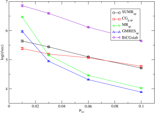
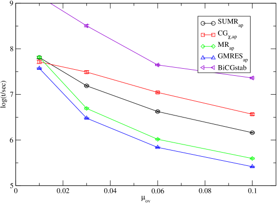
Figure 5: Average timings for the inversion of the overlap operator in units of seconds on a logarithmic scale for different bare quark masses. At $\beta=5.85$ on the $12^{4}$ (top) and the $16^{4}$ lattice (bottom).

We note that on the more relevant larger volume the pattern follows essentially the one observed for the numbers in table 6. As before, GMRES${}_{\text{ap}}$ and MR${}_{\text{ap}}$ appear to be more efficient than CG${}_{\chi,\text{ap}}$ and SUMR${}_{\text{ap}}$ except for very small quark masses. However, the almost perfect volume scaling of GMRES${}_{\text{ap}}$ (and similarly MR${}_{\text{ap}}$) suggests that these algorithms will break even also at small masses on large enough volumes. Indeed, as is evident from figure 5, this appears to be the case already on the $16^{4}$ lattice where we note that all four algorithms are similarly efficient with a slight advantage for the GMRES${}_{\text{ap}}$.

Let us conclude this section with the remark that a comparison of the above algorithms apparently depends very much on the detailed situation in which the algorithms are used and the specific viewpoint one takes. For example, the conclusion will be different for the reasons discussed above depending on whether a simulation is done on a large or intermediate lattice volume, or whether one is interested in small or intermediate bare quark masses. In a quenched or partially quenched calculation one will be interested in MM algorithms which e.g. would exclude the GMRES${}_{\text{ap}}$ and MR${}_{\text{ap}}$, on the other hand in a dynamical simulation this exclusion is only important when a RHMC algorithm is used [31, 32].

5.3.2 Low mode preconditioning

Let us now turn to low mode preconditioning. We concentrate on the non-hermitian LMP versions of GMRES${}_{\text{ap}}$ and MR${}_{\text{ap}}$ (cf. sec.4.2) and compare it to the hermitian LMP version of CG${}_{\text{ap}}$ [25] and in the following we denote the LMP version of the algorithms by the additional subscript ${}_{\text{lmp}}$. Both GMRES${}_{\text{ap,lmp}}$ and MR${}_{\text{ap,lmp}}$ are particularly promising since the un-preconditioned versions show a rather bad performance towards small quark masses, i.e. they fail to perform efficiently if the condition number of the operator $D$ gets too large. Obviously, projecting out the few lowest modes of $D$ and treating them exactly essentially keeps the condition number constant even when the bare quark mass is pushed to smaller values, e.g. into the $\varepsilon$–regime, and hence it has the potential to be particularly useful. Furthermore, we expect the iteration numbers to decrease for the LMP operators so that the overhead of GMRES and MR with respect to CG due to the way the adaptive precision is implemented becomes less severe.

The low modes are calculated using the methods described in appendix A. For the following comparison the normalised low modes $\psi^{(\pm)}_{k}$ of $A_{\pm}=P_{\pm}D^{\dagger}DP_{\pm}$ are calculated separately in each chiral sector up to a precision which is defined through the norm of the gradient $g^{(\pm)}_{k}$ in analogy to Eq.(14). For later convenience we introduce the triplet notation $(n_{0},n_{+},n_{-})$ to indicate the set of $n_{0}$ zero modes and $n_{\pm}$ modes in the chirally positive and negative sector, respectively. These eigenvectors can directly be used in the CG${}_{\text{ap,lmp}}$, but for the GMRES${}_{\text{ap,lmp}}$ and MR${}_{\text{ap,lmp}}$ one has to reconstruct the approximate (left and right) eigenvectors, eigenvalues and gradients. This is achieved by diagonalising the operator $D$ in the subspace spanned by the modes $\psi^{(\pm)}_{k}$ leading to Eq.(14) and (15).

At this point it appears to be important that the number of modes $n_{\pm}$ in the two chiral sectors match each other (up to zero modes of the massless operator) in order for the non-hermitian LMP to work efficiently. This is illustrated in figure 6 where we plot the square norm of the true residual $|r|^{2}$ of the preconditioned operator Eq.(25) against the iteration number of the GMRES${}_{\text{ap,lmp}}(10)$ algorithm at $\mu=0.005$ on a sample $16^{4}$ configuration with topological index $\nu=5$. The two full lines show the residuals in the case where the set $(5,10,10)$ is used while the dashed lines are the residuals obtained with the set (5,5,12). So in addition to the five zero modes, in the latter case only the first five non-zero modes of the non-hermitian operator can effectively be reconstructed while in the former case it is the first 10 non-zero modes leading to a much improved convergence. More severe, however, is the fact that the convergence may become unstable if the modes are not matched.

Figure 6: The square norm of the true residual $|r|^{2}$ of the LM preconditioned operator against the iteration number of the GMRES${}_{\text{ap,lmp}}(10)$ algorithm at $\mu=0.005$ on a sample $16^{4}$ configuration with topological index $\nu=5$. The full lines show the convergence when the modes of the two chiral sectors are matched, $n_{+}=n_{-}$, dashed lines when the modes are not matched, $n_{+}\neq n_{-}$. $\eta_{\pm}$ refers to the chirality of the point source.

In the example above we have used modes $\psi^{(\pm)}_{k}$ that were calculated with an accuracy $|g^{(\pm)}_{k}|^{2}\lesssim 10^{-4}$ which, after the reconstruction of the $l_{k}$ and $r_{k}$’s, translated into $|g^{(l,r)}_{k}|^{2}\simeq 5\cdot 10^{-3}$. It is surprising to see that the LMP works even with such a low accuracy of the low modes. On the other hand, after convergence of the LM preconditioned operator (cf. eq.(25)) and after adding in the contributions from the low modes (cf. eq.(26)), we find that there is a loss in the true residual of the full operator. This is illustrated in figure 7

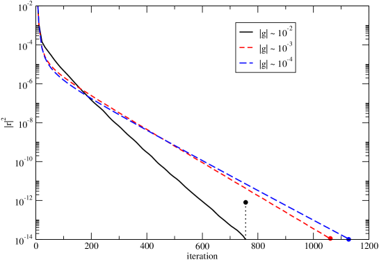
Figure 7: The square norm of the true residual $|r|^{2}$ of the LM preconditioned operator against the iteration number of the GMRES${}_{\text{ap,lmp}}(10)$ algorithm at $\mu=0.005$ on a sample $16^{4}$ configuration with topological index $\nu=5$. For the low mode set (5,10,10) calculated to an accuracy of $|g^{(\pm)}_{k}|^{2}\simeq 10^{-4}$ (solid black), $10^{-6}$ (short dashed red) and $10^{-8}$ (long dashed blue). The dot denotes the residual after adding in the contribution from the low modes.

where we show the square norm of the true residual $|r|^{2}$ of the LM preconditioned operator against the iteration number of the GMRES${}_{\text{ap,lmp}}(10)$ algorithm for the same configuration as before, using the set (5,10,10) calculated to an accuracy of $|g^{(\pm)}_{k}|\simeq 10^{-4}$ (solid black line) together with the true residual (filled black circle) after adding in the contribution from the low modes. On the other hand, if we use the set (5,10,10) calculated to an accuracy of $|g^{(\pm)}_{k}|\simeq 10^{-6}$ (short dashed red line) and $10^{-8}$ (long dashed blue line), the true residual can be sustained at $|r|^{2}\simeq 10^{-14}$ even after adding in the low mode contributions (filled circles). What is surprising, however, is that the version using the least accurate low modes converges the fastest, while the version using the most accurate low modes converges slowest.

Another point worth investigating is how the convergence depends on the number of projected modes. In figure 8 we show the convergence history for

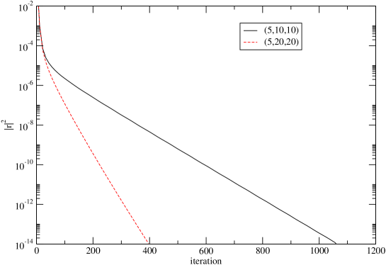
Figure 8: The square norm of the true residual $|r|^{2}$ of the LM preconditioned operator against the iteration number of the GMRES${}_{\text{ap,lmp}}(10)$ algorithm at $\mu=0.005$ on a sample $16^{4}$ configuration with topological index $\nu=5$. For the low mode set (5,10,10) (solid black line) and (5,20,20) (short dashed red line) matched low modes calculated to an accuracy of $|g^{(\pm)}_{k}|^{2}\simeq 10^{-6}$.

the GMRES${}_{\text{ap,lmp}}(10)$ algorithm in the case when the set (5,10,10) (solid black line) and (5,20,20) (short dashed red line) of low modes calculated to an accuracy of $|g^{(\pm)}_{k}|^{2}\simeq 10^{-6}$ are used for the preconditioning. In both cases the convergence is approximately exponential with exponents 0.0195 and 0.056 for the preconditioning with (5,10,10) and (5,20,20) modes, respectively, and the ratio of exponents matches precisely the ratio of the squared condition numbers of the preconditioned operators. Finally we note that there is no sensitivity to whether or not the source is in the chiral sector which contains the zero-modes.

In fig.9 we show the average timings for the inversion of the LM preconditioned overlap operator. For the LMP in addition to the zero modes we have used 10 nonzero modes on both volumes, i.e. the set $(n_{0},10,10)$. Obviously, to achieve similar improvement on different volumes one should scale the number of low modes with the volume. The fact that we have not done so is reflected in the degradation of the algorithm performance on the larger volume towards smaller quark mass, but one should keep in mind that the improvement w.r.t. the un-preconditioned operator can be easily enhanced by using more low modes.

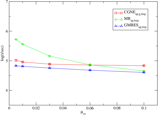
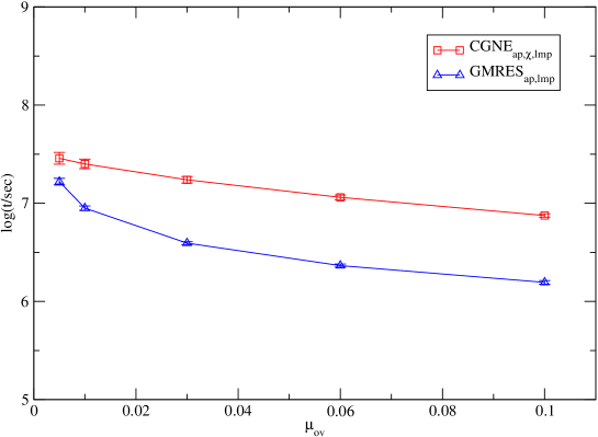
Figure 9: Average timings for the inversion of the low mode preconditioned overlap operator in units of seconds for different bare quark masses. At $\beta=5.85$ on the $12^{4}$ (top) and the $16^{4}$ lattice (bottom).

The scale is chosen so that the figures can be directly compared to the ones in fig.5, but we remark that such a comparison is only of limited interest, since the improvement w.r.t. the un-preconditioned operator will depend strongly on the number of low modes and the quark mass.

The timings include all the preparation of the eigenmodes as described in section 5.3.2. Comparing the results for the highest mass with the ones in fig.5 it becomes clear that the preparation amounts to a non-negligible fraction of the total time, but it should be noted that in a real production it has to be done only once for all inversions on a given configuration.

In conclusion we find that GMRES${}_{\text{ap,lmp}}$ outperforms CG${}_{\text{ap,lmp}}$ by factors of up to two in the range of parameters investigated here. Due to the favourable volume scaling of the GMRES${}_{\text{ap,lmp}}$ algorithm this factor is expected to become even larger on larger volumes.

5.4 Comparison between overlap and Wilson TM

The results of the previous sections emphasise that an investigation like the present one is worthwhile – for both the overlap and the twisted mass operator the relative cost factor between the worst and the best algorithm can be as much as one order of magnitude.

Let us compare directly the absolute and relative cost for the overlap and twisted mass operator in table 7 and table 8 where we pick in each case the best available algorithm, GMRES${}_{\text{ap}}$ for the overlap and CGS${}_{\text{eo}}$ for the twisted mass operator. We observe that the relative factor in the cost (measured in execution time or MV products) lies between 30 for the heaviest mass under investigation and 120 for the lightest mass. The pattern appears to be similar for the two volumes we looked at, even though the relative factor is slightly increasing with the volume.

$V,m_{\pi}$[MeV]	Wilson TM	overlap	rel. factor
$12^{4},720$	599	18.1	30
555	774	27.9	36
390	944	52.9	56
230	1048	96.7	92
$16^{4},720$	650	22.3	34
555	962	34.5	36
390	1317	66.0	50
230	1687	198.5	118

Table 7: Number of $Q$ applications for the best available algorithm and the corresponding relative cost factor. For the overlap operator the number of $Q$ applications is in units of 1000.

$V,m_{\pi}$[MeV]	Wilson TM	overlap	rel. factor
$12^{4},720$	1.0	48.8	49
555	1.3	75.1	58
390	1.6	141.5	88
230	1.8	225.0	125
$16^{4},720$	3.7	225.3	61
555	5.2	343.9	66
390	6.8	652.7	96
230	10.0	1949.3	195

Table 8: Absolute timings in seconds on one node of JUelich MultiProzessor (JUMP) IBM p690 Regatta in Jülich for the best available algorithm and the corresponding relative cost factor.

We would like to emphasise that the overlap operator as used in this paper obeys lattice chiral symmetry up to machine precision and hence the relative factor compared to TM fermions will be less if a less stringent Ginsparg-Wilson fermion is used. Including those fermions as well as improved overlap fermions (for instance with a smeared kernel) in the tests are, however, beyond the scope of this paper.

6 Conclusions and Outlook

In this paper we have performed a comprehensive, though not complete test of various algorithms to solve very large sets of linear systems employing sparse matrices as needed in applications of lattice QCD. We considered two relatively new formulations of lattice QCD, chirally improved Wilson twisted mass fermions at full twist and chirally invariant overlap fermions. The tests were performed on $12^{4}$ and $16^{4}$ lattices and four values of the pseudo scalar mass of 230MeV, 390MeV, 555MeV and 720MeV. The lattice spacing has been fixed to $a\approx 0.125$fm.

We think that our study will help to select a good linear system solver for twisted mass and overlap fermions for practical simulations. We emphasise that we cannot provide a definite choice of the optimal algorithm for each case. The reason simply is that the optimal choice depends on many details of the problem at hand such as the exact pseudo scalar mass, the volume, the source vector etc.. Nevertheless, in general we find that for twisted mass fermions CGS appears to be the fastest linear solver algorithm while for overlap fermions it is GMRES${}_{\text{ap}}$ for the parameters investigated here. In a direct competition between twisted mass and overlap fermions the latter are by a factor of 30-120 more expensive if one compares the best available algorithms in each case with an increasing factor when the value of the pseudo scalar mass is lowered. Preconditioning plays an important role for both investigated fermion simulations. A factor of two is obtained by using even/odd preconditioning for the TM operator. A similar improvement can be expected from SSOR preconditioning [33, 34].

For the overlap operator it turns out to be rather efficient to adapt the precision of the polynomial approximation in the course of the solver iterations. This easily speeds up the inversion by a factor of two. In the $\epsilon$-regime in addition low mode preconditioning can overcome the slowing down of the convergence of the algorithms towards small quark masses and the convergence rate can essentially be kept constant for all masses. In particular we find that the GMRES${}_{\text{ap,lmp}}$ outperforms CG${}_{\text{ap,lmp}}$ by factors of up to two with tendency of getting even better towards larger volumes.

One of the aims of this paper has been to at least start an algorithm comparison and we would hope that our study here will be extended by other groups adding their choice of algorithm, optimally using the here employed simulations parameters as benchmark points. In this way, a toolkit of algorithms could be generated and gradually enlarged.

Appendix A Eigenpair Computation

As mentioned already in section 2, the computation of eigenvalues and eigenvectors or approximations of those are needed in various methods used in this paper, e.g. for the practical implementation of the $\operatorname{sign}$-function or the low mode preconditioning of the overlap operator. But also if one is interested in computing the topological index with the overlap operator one needs an algorithm to compute the eigenvalues of the overlap operator.

The standard method used in lattice QCD is the so called Ritz-Jacobi method [35]. For the use of adaptive precision for the overlap operator with this method, see Ref. [36, 25]. Another choice would be the Arnoldi algorithm implemented in the ARPACK package which, however, sometimes fails to compute for instance a given number of the lowest eigenvalues of $Q^{2}$ by missing one. This might lead to problems if the eigenvalues are used to normalise the Wilson-Dirac operator in the polynomial construction of the overlap operator.

We used yet another method which is described in the following section. After that we present some implementation details for the determination of the index.

A.1 Jacobi-Davidson method

Consider a complex valued $N\times N$ matrix $A$ for which we aim at determining (part of) its eigenvalues and eigenvectors. The exact computation of those is in general too demanding and thus one has to rely on some iterative method. The one we are going to describe here was introduced in [37].

Assume we have an approximation $(\lambda_{k},u_{k})$ for the eigenpair $(\lambda,u)$ and we want to find a correction $v$ to $u_{k}$ in order to improve the approximation. One way of doing this is to look for the orthogonal complement for $u_{k}$ with respect to $u$, which means we are interested in the subspace $u_{k}^{\perp}$.

The projection of $A$ into this subspace is given by

$$B_{k}\equiv(I-u_{k}u_{k}^{\dagger})A(I-u_{k}u_{k}^{\dagger})\,,$$ (27)

where the vector $u_{k}$ has been normalised and $I$ represents the identity matrix. Eq. (27) can be rewritten as follows

$$A=B_{k}+Au_{k}u_{k}^{\dagger}+u_{k}u_{k}^{\dagger}A-\lambda_{k}u_{k}u_{k}^{\dagger}\,.$$ (28)

Since we want to find $v\perp u_{k}$ such that

$$A(u_{k}+v)=\lambda(u_{k}+v)\,,$$

it follows with $B_{k}u_{k}=0$

$$(B_{k}-\lambda I)v=-r_{k}+(\lambda-\lambda_{k}-u_{k}^{\dagger}Av)u_{k}\,,$$ (29)

where we introduced the residual vector $r_{k}$ given by

$$r_{k}=(A-\lambda_{k}I)u_{k}\,.$$

Neither $r_{k}$ nor the l.h.s of Eq. (29) have a component in direction $u_{k}$ and hence $v$ should satisfy

$$(B_{k}-\lambda I)v=-r_{k}\,.$$ (30)

Since $\lambda$ is unknown, we replace it by $\lambda_{k}$ and Eq. (30) can then be solved with any iterative solver. Note that the matrix $B$ depends on the approximation $u_{k}$ and needs to be newly constructed in every step.

Solving Eq. (30) for $v$ in every iteration step might look as if the proposed algorithm is rather computer time demanding. But it turns out that in fact it has to be solved only approximately, i.e. in each iteration step only a few iterations of the solver have to be performed.

Algorithm 3 Basic Jacobi-Davidson algorithm

0:  non trivial initial guess vector $v$, $m>1$

1:  $v_{1}=v/\|v\|$, $w_{1}=Av_{1}$, $h_{11}=v_{1}^{\dagger}w_{1}$, $i=1$

2:  $V_{1}=\{v_{1}\}$, $W_{1}=\{w_{1}\}$, $H_{1}=\{h_{11}\}$

3:  $u_{k}=v_{1}$, $\lambda_{1}=h_{11}$

4:  $r_{1}=w_{1}-\lambda_{1}u$

5:  repeat

6:     for $k=1,...,m-1$ do

7:        solve approximately for $v_{k+1}\perp u_{k}$

$$(I-u_{k}u_{k}^{\dagger})(A-\lambda_{k}I)(I-u_{k}u_{k}^{\dagger})v_{k+1}=-r_{k}$$ (31)

8:        orthogonalise $v_{k+1}$ against $V_{k}$, $V_{k+1}=\{V_{k},v_{k+1}\}$

9:        $w_{k+1}=Av_{k+1}$, $W_{k+1}=\{W_{k},w_{k+1}\}$

10:        compute $V_{k+1}^{\dagger}w_{k+1}$, the last column of $H_{k+1}\equiv V_{k+1}^{\dagger}AV_{k+1}$

11:        if $A$ is not hermitian then

12:           compute $v_{k+1}^{\dagger}W_{k}$, the last row of $H_{k+1}$

13:        end if

14:        compute the smallest eigenpair $(\lambda_{k+1},s)$ of $H_{k+1}$ and normalise $s$.

15:        $u_{k+1}=V_{k+1}s\quad$ // The new eigenvector approximation

16:        $\hat{u}=Au_{k+1}$ and $r_{k+1}=\hat{u}-\lambda_{k+1}u_{k+1}$

17:        test for convergence, $i=i+1$

18:     end for

19:     restart: Set $V_{1}=\{u_{m}\}$, $W_{1}=\{\hat{u}\}$, $H_{1}=\{\lambda_{m}\}$

20:  until convergence

The basic Jacobi-Davidson (JD) algorithm is summarised in algorithm 3. In algorithm 3 we denote matrices with capital letters and vectors with small letters. $V=\{v\}$ means that the matrix $V$ contains only one column $v$, while $W=\{V,v\}$ means that $V$ is expanded by $v$ to the matrix $W$ by one column. The basic algorithm can be easily extended in order to compute more than the minimal (maximal) eigenvalue: the simplest way is to perform a restart and restrict the eigenvector search to the subspace orthogonal to the already computed eigenvector(s).

A further way to compute more than one eigenvalue is to solve Eq. (30) more than once per iteration for several approximate eigenvectors. This so called blocking method is also capable to deal with degenerate eigenvalues, which are otherwise not correctly computed by the JD method [38, 39].

Moreover, the JD algorithm is able to compute eigenpairs which are located in the bulk eigenvalue spectrum of $A$. This is achieved by replacing $\lambda_{k}$ in Eq. (30) by an initial guess $\sigma$ in the first few iterations, which will drive the JD algorithm to compute preferably eigenvalues close to $\sigma$ [37].

Let us finally discuss some implementation details regarding the parallelisation of the JD algorithm. As soon as the application of $A$ is parallelised most of the remaining linear algebra operations are parallelised trivially, which includes matrix-vector multiplications as $V_{k+1}^{\dagger}w_{k+1}$. Only the computation of the eigenvalues of the (low dimensional) matrix $H$ is not immediately parallelisable and, in fact, it is most efficient to hold a local copy of $H$ and compute the eigenvalues on each processor. Then the multiplication $V_{k+1}s$ in line $15$ of algorithm 3 is even a local operation. This seems to be a doubling of work, but as $H$ is only an order $20\times 20$ matrix, the parallelisation overhead would be too large.

A.1.1 Index computation

The computation of the topological index on a given gauge configuration with the overlap operator involves counting the zero modes of $D_{\mathrm{ov}}$. More precisely, the chiral sector containing zero modes has to be identified and then their number has to be determined. To this end we have implemented the method of Ref. [25] which makes use of the Ritz-Jacobi algorithm. Moreover, it is straightforward to adapt the method also to the JD algorithm. So we are not going to mention the details of this algorithm.

But it is useful to discuss some performance improvements of the index computation: the most time consuming part in the JD algorithm is to find an approximate solution to Eq. (30). As suggested in Refs. [38, 39], we used the following set-up. The actual absolute precision to which the solution is driven is computed as

$$\epsilon=x^{-i}\,,$$

where $i$ counts the number of JD-iterations performed so far for the eigenvalue in question (see algorithm 3) and $x=1.5$. Additionally we set the maximal number of iterations in the solver to $50$. In this way we avoid on the one hand that the solution to Eq. (30) is much more precise than the current approximation for the eigenvalue and on the other hand too many iterations in the solver.

Thus, most of the time, the precision required from the iterative solver is only rough, and hence it is useful to use adaptive precision for the $\operatorname{sign}$-function, since the polynomial approximation of the $\operatorname{sign}$-function is not needed to be much more precise than the required solver precision. Our experience shows that setting the precision in the polynomial to $10^{-2}\cdot\epsilon$ is a good choice in this respect. We remark that the vector $w_{k+1}$ (see line $9$ in algorithm 3) as well as the next residual $r_{k+1}$ should be computed with full precision in the polynomial in order not to bias the computation.

A.2 Index from the CG search

For the computation of the topological index it is important to note that the determination of the chiral sector which contains the zero-modes comes for free when one uses the CG-algorithm for the inversion. By estimating the eigenvalues once in each chiral sector and by pairing them accordingly it is possible to identify the chiral sector which contains zero modes. From the CG-coefficients which are obtained during the iteration one can build up a tridiagonal matrix which is related to the underlying Lanczos procedure [9]. The eigenvalues of this matrix approximate the extremal eigenvalues of the operator and it turns out that the lowest 5-10 eigenvalues are approximated rather accurately.

In figure 10 we plot the iterative determination of the lowest eigenvalues during a CG-inversion for two different configurations. For the first configuration (left plot) we see a rapid convergence of the unpaired lowest eigenvalue towards the zero mode value suggesting a non-zero topological charge in the given chiral sector. The second configuration on the other hand (right plot) also shows a rapid convergence of the lowest mode towards the zero mode value, but this time it is paired by an equal eigenvalue in the opposite chiral sector hence suggesting a configuration with zero topological charge. Figure 10 emphasises the point that the pairing of modes in the two chiral sectors is the crucial ingredient for the determination of the topological charge sector and not the estimate of the eigenvalue itself. Indeed, for the second configuration the eigenvalue estimates converge to a value slightly larger than the zero mode value as one would expect.

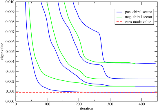
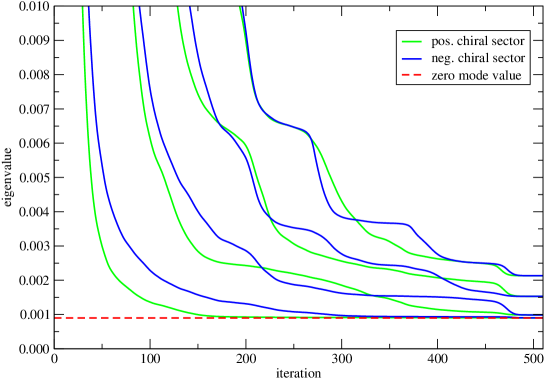
Figure 10: Estimates of the lowest eigenvalues of the overlap operator from the CG-coefficients for a $16^{4}$ configuration with topological charge $\nu<0$ (top) and $\nu=0$ (bottom) at $\mu_{\textrm{ov}}=0.03$.

Appendix B Multiple mass solver for twisted mass fermions

We want to invert the TM operator at a certain twisted mass $\mu_{0}$ obtaining automatically all the solutions for other twisted masses $\mu_{k}$ (with $|\mu_{k}|\geq|\mu_{0}|$). Then, as in Eq.(3) the Wilson twisted mass operator is

$$D_{\rm tm}=D_{\mathrm{W}}+i\mu_{k}\gamma_{5}\tau^{3},\qquad k=1,\ldots,N_{m}$$ (32)

where $N_{m}$ is the number of additional twisted masses. The operator can be split as

$$D_{\rm tm}=D_{\rm tm}^{(0)}+i(\mu_{k}-\mu_{0})\gamma_{5}\tau^{3},\qquad D_{\rm tm}^{(0)}=D_{\mathrm{W}}+i\mu_{0}\gamma_{5}\tau^{3}$$ (33)

The trivial observation is that

$$D_{\rm tm}D_{\rm tm}^{\dagger}=D_{\rm tm}^{(0)}D_{\rm tm}^{(0)\dagger}+\mu_{k}^{2}-\mu_{0}^{2}\;,$$ (34)

where we have used $\gamma_{5}D_{\mathrm{W}}\gamma_{5}=D_{\mathrm{W}}^{\dagger}$. Now clearly we have a shifted linear system $(A+\sigma_{k})x-b=0$ with $A=D_{\rm tm}^{(0)}D_{\rm tm}^{(0)\dagger}$ and $\sigma_{k}=\mu_{k}^{2}-\mu_{0}^{2}$. In algorithm 4 we describe the CG-M algorithm to solve the problem $(A+\sigma_{k})x-b=0$. The lower index indicates the iteration steps of the solver, while the upper index $k$ refers to the shifted problem with $\sigma_{k}$. The symbols without upper index refer to mass $\mu_{0}$.

Algorithm 4 CG-M algorithm

1:  $n=0,x_{0}^{k}=0,r_{0}=p_{0}=p_{0}^{k}=b$

2:  $\biggl{.}\biggr{.}\alpha_{-1}=\zeta_{-1}^{k}=\zeta_{0}^{k}=1,\beta_{0}^{k}=\beta_{0}=0$

3:  repeat

4:     $\alpha_{n}=(r_{n},r_{n})/(p_{n},Ap_{n})$

5:     $\biggl{.}\biggr{.}\zeta_{n+1}^{k}=(\zeta^{k}_{n}\alpha_{n-1})/(\alpha_{n}\beta_{n}(1-\zeta_{n}^{k}/\zeta^{k}_{n-1})+\alpha_{n-1}(1-\sigma_{k}\alpha_{n}))$

6:     $\alpha^{k}_{n}=(\alpha_{n}\zeta_{n+1}^{k})/\zeta_{n}^{k}$

7:     $\biggl{.}\biggr{.}x_{n+1}^{k}=x_{n}^{k}+\alpha_{n}^{k}p_{n}^{k}$

8:     $x_{n+1}=x_{n}+\alpha_{n}p_{n}$

9:     $\biggl{.}\biggr{.}r_{n+1}=r_{n}-\alpha_{n}Ap_{n}$

10:     $\beta_{n+1}=(r_{n+1},r_{n+1})/(r_{n},r_{n})$

11:     $\biggl{.}\biggr{.}p_{n+1}^{k}=\zeta_{n+1}^{k}r_{n+1}+\beta_{n+1}^{k}p_{n}^{k}$

12:     $n=n+1$

13:  until $\|r_{n}\|<\epsilon$

References

- [1] M. Lüscher, Phys. Lett. B428, 342 (1998), [hep-lat/9802011].
- [2] H. Neuberger, Phys. Lett. B417, 141 (1998), [hep-lat/9707022].
- [3] H. Neuberger, Phys. Lett. B427, 353 (1998), [hep-lat/9801031].
- [4] R. Frezzotti and G. C. Rossi, JHEP 08, 007 (2004), [hep-lat/0306014].
- [5] LF , W. Bietenholz et al., JHEP 12, 044 (2004), [hep-lat/0411001].
- [6] CP-PACS and JLQCD, A. Ukawa, Nucl. Phys. Proc. Suppl. 106, 195 (2002).
- [7] K. Jansen, Nucl. Phys. Proc. Suppl. 129, 3 (2004), [hep-lat/0311039].
- [8] C. Urbach, K. Jansen, A. Shindler and U. Wenger, Comput. Phys. Commun. 174, 87 (2006), [hep-lat/0506011].
- [9] Y. Saad, Iterative Methods for sparse linear systems, 2nd ed. (SIAM, 2003).
- [10] A. Frommer, B. Nockel, S. Gusken, T. Lippert and K. Schilling, Int. J. Mod. Phys. C6, 627 (1995), [hep-lat/9504020].
- [11] T. Chiarappa et al., Nucl. Phys. Proc. Suppl. 140, 853 (2005), [hep-lat/0409107].
- [12] G. Arnold et al., hep-lat/0311025.
- [13] N. Cundy et al., Comput. Phys. Commun. 165, 221 (2005), [hep-lat/0405003].
- [14] S. Krieg et al., Nucl. Phys. Proc. Suppl. 140, 856 (2005), [hep-lat/0409030].
- [15] R. Frezzotti, P. A. Grassi, S. Sint and P. Weisz, Nucl. Phys. Proc. Suppl. 83, 941 (2000), [hep-lat/9909003].
- [16] ALPHA, R. Frezzotti, P. A. Grassi, S. Sint and P. Weisz, JHEP 08, 058 (2001), [hep-lat/0101001].
- [17] LF , K. Jansen, A. Shindler, C. Urbach and I. Wetzorke, Phys. Lett. B586, 432 (2004), [hep-lat/0312013].
- [18] LF , K. Jansen, M. Papinutto, A. Shindler, C. Urbach and I. Wetzorke, JHEP 09, 071 (2005), [hep-lat/0507010].
- [19] C. F. Jagels and L. Reichel, Numer. Linear Algebra Appl. 1(6), 555 (1994).
- [20] Y. Saad, SIAM J. Sci. Comput. 14 (2) (1993).
- [21] U. Glässner et al., hep-lat/9605008.
- [22] B. Jegerlehner, hep-lat/9612014.
- [23] F. Jegerlehner, Nucl. Phys. Proc. Suppl. 126, 325 (2004), [hep-ph/0310234].
- [24] R. G. Edwards, U. M. Heller and R. Narayanan, Phys. Rev. D59, 094510 (1999), [hep-lat/9811030].
- [25] L. Giusti, C. Hoelbling, M. Lüscher and H. Wittig, Comput. Phys. Commun. 153, 31 (2003), [hep-lat/0212012].
- [26] F. Farchioni et al., Eur. Phys. J. C39, 421 (2005), [hep-lat/0406039].
- [27] K. Jansen and C. Liu, Comput. Phys. Commun. 99, 221 (1997), [hep-lat/9603008].
- [28] K. Burrage and J. Erhel, Num. Lin. Alg. with Appl. 5, 101 (1998).
- [29] R. B. Morgan, SIAM J. Sci. Comput. 24, 20 (2002).
- [30] P. Sonneveld, SIAM J. Sci. Stat. Comput. 10, 36 (1989).
- [31] M. A. Clark, P. de Forcrand and A. D. Kennedy, PoS LAT2005, 115 (2005), [hep-lat/0510004].
- [32] M. A. Clark and A. D. Kennedy, hep-lat/0608015.
- [33] S. Fischer et al., Comp. Phys. Commun. 98, 20 (1996), [hep-lat/9602019].
- [34] A. Frommer, V. Hannemann, B. Nockel, T. Lippert and K. Schilling, Int. J. Mod. Phys. C5, 1073 (1994), [hep-lat/9404013].
- [35] T. Kalkreuter and H. Simma, Comput. Phys. Commun. 93, 33 (1996), [hep-lat/9507023].
- [36] N. Cundy, M. Teper and U. Wenger, Phys. Rev. D66, 094505 (2002), [hep-lat/0203030].
- [37] G. L. G. Sleijpen and H. A. V. der Vorst, SIAM Journal on Matrix Analysis and Applications 17, 401 (1996).
- [38] D. R. Fokkema, G. L. G. Sleijpen and H. A. Van der Vorst, J. Sci. Comput. 20, 94 (1998).
- [39] R. Geus, The Jacobi-Davidson algorithm for solving large sparse symmetric eigenvalue problems with application to the design of accelerator cavities, PhD thesis, Swiss Federal Institute Of Technology Zürich, 2002.