Trajectory Length and Autocorrelation Times – $N_{f}=2$ simulations in the Schrödinger functional

Abstract:

A status report is presented on the large-volume simulations in the Schrödinger functional with two flavours of O($a$) improved Wilson quarks performed by the ALPHA collaboration. The physics goal is to set the scale for the computation of the fundamental parameters of QCD. In this talk the emphasis is on aspects of the Hybrid Monte-Carlo algorithm, which we use with (symmetric) even-odd and Hasenbusch preconditioning. We study the dependence of aucorrelation times on the trajectory length. The latter is found to be significant for fermionic correlators, the trajectories longer than unity performing better than the shorter ones.
DESY 06-161
HU-EP-06/28
SFB/CPP-06-42

1 Motivation

Recently the $\Lambda$-parameter of two-flavour QCD has been computed by the ALPHA collaboration in the Schrödinger functional scheme in units of a low-energy scale $\mathop{L_{\rm max}}$ [1]. The latter scale is defined implicitly by the renormalized coupling in that scheme taking a particular value, $\bar{g}^{2}_{\rm SF}(\mu=1/L)=4.61$. The determined quantity $\Lambda_{\rm SF}\mathop{L_{\rm max}}$ is a continuum, universal result. The connection between $\Lambda_{\rm SF}$ and $\mathop{\Lambda_{\overline{\rm MS}}}$ being known exactly [2], what remains to be done, for the result to be phenomenologically useful, is to trade $\mathop{L_{\rm max}}$ for an experimentally accessible low-energy scale. This was done provisionnally [1] using the chirally extrapolated Sommer reference scale $r_{0}$ [3, 1], however choosing a more directly accessible physical quantity will reduce the systematic uncertainty. Our present goal is to use the kaon decay constant $F_{K}$ as low-energy scale. This will also allow us to reduce the overall uncertainty on our recent determination of the strange quark mass [4].

More specifically, a possible strategy is to compute $\mathop{L_{\rm max}}\mathop{F_{\rm ps}}$ at a tuned quark mass such that $\frac{\mathop{M_{\rm ps}}}{\mathop{F_{\rm ps}}}(\mathop{m_{\rm ref}},\mathop{m_{\rm ref}})=\frac{M_{K}}{F_{K}}|_{\rm exp}$. Neglecting the quenching of a third quark of mass $\mathop{m_{\rm ref}}$, SU(3) chiral perturbation theory then connects $\mathop{F_{\rm ps}}(\mathop{m_{\rm ref}},\mathop{m_{\rm ref}},\mathop{m_{\rm ref}})$ to $\mathop{F_{\rm ps}}(m_{u},m_{d},m_{s})$, which is equated to its experimental value of $113{\rm MeV}$. At one-loop level [5], with $\mu_{P}=\textstyle{\frac{M_{P}^{2}}{32\pi^{2}F_{0}^{2}}}~{}\log\{M_{P}^{2}/\mu^{2}\}$ and $F_{0}=88$MeV we have

$$\frac{\mathop{m_{\rm ref}}}{(m_{\ell}+m_{s})/2} = 1+\textstyle{\frac{3}{2}}\mu_{\pi}-\textstyle{\frac{11}{3}}\mu_{K}+\textstyle{\frac{13}{6}}\mu_{\eta}+\frac{16}{F_{0}^{2}}[L_{4}(\mu)-L_{6}(\mu)]\cdot[M_{K}^{2}-M_{\pi}^{2}]$$

$$= 1~{}+~{}0.10~{}+~{}0.47\cdot 10^{3}[L_{4}(M_{\rho})-L_{6}(M_{\rho})],$$

$$\frac{\mathop{F_{\rm ps}}(\mathop{m_{\rm ref}},\mathop{m_{\rm ref}},\mathop{m_{\rm ref}})}{F_{K}(m_{\ell},m_{\ell},m_{s})} = 1+\textstyle{\frac{3}{4}}(\mu_{\pi}-2\mu_{K}+\mu_{\eta})+\textstyle{\frac{4}{F_{0}^{2}}}\cdot L_{4}(\mu)\cdot[M_{K}^{2}-M_{\pi}^{2}]$$

$$= 1~{}+~{}0.051~{}+~{}0.12\cdot 10^{3}L_{4}(M_{\rho}),$$

where phenomenological studies point to $10^{3}|L_{4}|\leq 1$ and $0.2\leq 10^{3}[L_{4}(M_{\rho})-L_{6}(M_{\rho})]\leq 0.4$ [6, 7]. These ranges can be narrowed down by lattice simulations. Using the tree-level relation $4M_{K}^{2}-3M_{\eta}^{2}=M_{\pi}^{2}$, it can be verified that the dependence on $\mu$ cancels in Eq. (1) and (1).

Although the original purpose of the Schrödinger functional was to provide the setting for the implementation of a finite-volume renormalization scheme, it was shown [8] in the quenched approximation that it also provides a competitive tool for spectrum and matrix element calculations. Roughly speaking, the Dirichlet boundary conditions in the time directions are now exploited in the same way as in the source method that was used in the early days of glueball spectroscopy [9].

2 Simulations at $\mathop{m_{\rm ref}}$

We use the ${N_{\rm f}}=2$ O($a$) improved Wilson formulation with plaquette gauge action $S_{\rm g}$. Our simulations are performed with the Hybrid Monte-Carlo algorithm with (symmetric) even-odd [10] and Hasenbusch preconditioning [11]. The action thus reads $S=S_{\rm pf}~{}+~{}S_{\det}~{}+~{}S_{\rm g}$, with

$$S_{\rm pf}=\phi_{0}^{\dagger}\frac{1}{\hat{Q}\hat{Q}^{\dagger}+\rho_{0}^{2}M_{\rm oo}^{-2}}\phi_{0}+\sum_{k=1}^{n-1}\phi_{k}^{\dagger}\left(\frac{1}{\sigma_{k}^{2}}+\frac{1}{\hat{Q}_{A}^{2}+\rho_{k}^{2}}\right)\phi_{k}$$ (3)

where the pseudofermions (PFs) ‘live’ on the odd sites only and, in the notation of [10],

$$\hat{Q}_{A} = \gamma_{5}(M_{\rm oo}-M_{\rm oe}M^{-1}_{\rm ee}M_{\rm eo}),\qquad\hat{Q}=M^{-1}_{\rm oo}\hat{Q}_{A},$$ (4)

$$S_{\det} = (-2)\log\det M_{\rm ee}~{}+~{}(-2)\log\det M_{\rm oo},$$ (5)

The parameters $(\sigma_{k},\rho_{k})$ satisfy

$$\sigma_{k}^{2}=\rho_{k-1}^{2}-\rho_{k}^{2},\qquad k=1,\dots n-1;\qquad\rho_{n-1}=0.$$ (6)

The Hermitian matrix $\hat{Q}_{A}$ is thus the Schur complement of $Q\equiv\gamma_{5}D$ with respect to even-odd preconditioning. Note that $\hat{Q}$ on the other hand is not Hermitian. The matrices $M_{\rm oo},M_{\rm ee}$ are diagonal with respect to space indices, and their determinants are thus represented exactly on each configuration. All the simulations presented here are with $n=2$ unless otherwise stated.

2.1 Recent algorithmic improvements

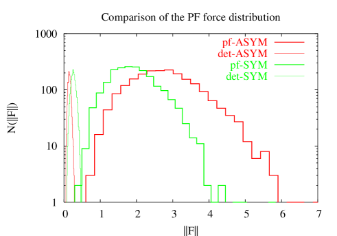
Figure 1: Comparison of the pseudofermion and determinant forces in the time-slice $T/2$ with symmetric and asymmetric even-odd preconditioning on an $8^{4}$ lattice at $\beta=6.32$ ($n=1$ here, and the normalization of the force is as in [18]).

The advantage of the symmetric form of even-odd preconditioning was first demonstrated in [12] with $n=1$. See [13] for a study with $n=2$ (where the shift $\rho$ was however implemented on $D$ rather than $Q$). We find that on a $16^{4}$ lattice at $\beta=5.2$, the stepsize $\delta\tau$ can be increased from $1/28$ to $1/20$ at a constant acceptance above $90\%$, when switching from the asymmetric to the symmetric form. This is easily explained by a reduction in the magnitude of the force, as illustrated on Fig. 1 for a small system. The operator $\hat{Q}$ is better behaved in the ultraviolet than $\hat{Q}_{A}$; the improvement is thus not expected to depend strongly on the size of the system. Secondly, in the Hamiltonian and force computation, the equation $(\hat{Q}_{A}^{2}+\rho^{2})\psi=\phi$ arises, to be solved for $\psi$. We then proceed as follows, with $M^{-1}_{\rm oo}$ stored:

$$\tilde{\phi}=M^{-1}_{\rm oo}\phi,\qquad(\hat{Q}-i\rho M^{-1}_{\rm oo})(\hat{Q}^{\dagger}+i\rho M^{-1}_{\rm oo})\tilde{\psi}=\tilde{\phi},\qquad\psi=M^{-1}_{\rm oo}\tilde{\psi}.$$ (7)

We use the conjugate gradient algorithm for the inversion involving $\hat{Q}$, and on the $16^{4}$ lattice find about a $20\%$ reduction in the number of iterations necessary to solve the equation with $\rho=0$ for a given target accuracy with respect to solving the equation involving $\hat{Q}_{A}$. Thus the symmetric variant is also a superior solver preconditioner as compared to the asymmetric one.

It was recently suggested to introduce a separate step-size $\delta\tau_{k}$ for each pseudofermion [14, 15] (a smaller step-size for the gauge force has been in use for a long time [16]). With $n=2$ one then has one additional parameter to tune, and it turns out that the simultaneous optimization of $\rho_{0}$ and $\delta\tau_{0}/\delta\tau_{1}$ leads to significantly smaller values of $\rho_{0}$ [15, 17] than if one constrains $\delta\tau_{0}=\delta\tau_{1}$. We find a gain resulting from the introduction of the extra parameter of about 1.5 on a $24^{3}\times 32$ lattice at $m\simeq\mathop{m_{\rm ref}}$, while no observable improvement could be obtained on the $16^{4}$, $\beta=5.2$ lattice. This suggests that the gain increases with the condition number of $\hat{Q}$.

We have also explored ‘hybrid’ integrators, where the leap-frog integration scheme is used for the force associated with $\phi_{1}$ and the Sexton-Weingarten [16] for that associated with $\phi_{0}$, and found the performance to be comparable. The motivation is to benefit from the robustness of the leap-frog integrator for the most irregular force to insure stability, while using a higher order scheme for the smoother forces.

3 Trajectory length dependence of autocorrelation times

We report some results on the algorithm figure-of-merit $\nu$ introduced in [18], which we generalize to any observable $O$. If $\tau_{\rm int}[O]$ is its autocorrelation time in units of trajectories, we have

$$\nu[O]\equiv 10^{-3}\cdot N_{\rm eff}^{\rm solver~{}calls}\cdot\tau_{\rm int}[O].$$ (8)

By ‘effective number of solver calls’, we mean the number of times the equation $\hat{Q}_{A}^{2}\psi=\phi$ has to be solved per trajectory, plus the number of times the equation $(\hat{Q}_{A}^{2}+\rho_{0}^{2})\psi=\phi$ has to be solved, weighted by the number of solver iterations this takes relative to the former equation. It turns out that these two contributions are roughly equal. The values of $\nu$ for the plaquette, the effective pion mass and pseudoscalar decay constant in the middle time-slice are given in Tab. 1. There is certainly no sign that the algorithm’s performance worsens as the quark mass decreases in the explored region. The figures for the plaquette $P$ are very similar to the ones quoted in [19], and also in [15] (if one uses the same definition of $N_{\rm eff}^{\rm solver~{}calls}$).

$\kappa$	$\tau$	integrator	$\delta\tau_{1}/\delta\tau_{0}$	$\nu[P]$	$\nu[\mathop{M_{\rm ps}}(T/2)]$	$\nu[\mathop{f_{\rm ps}}(T/2)]$
0.1355	$1/2$	SW	1	$0.47(13)$	$0.67(18)$	$1.4(5)$
0.1355	2	SW	1	$0.80(16)$	$0.65(16)$	$0.33(8)$
0.1359	$1/2$	SW	1	$0.36(8)$	$0.75(21)$	$0.45(10)$
0.13605	2	LF	5	$0.6(2)$	$0.25(6)$	$0.26(7)$
0.13625	2	LF	5	$0.55(27)$	$0.17(6)$	$0.16(6)$

Table 1: The figure-of-merit $\nu[O]$ for the plaquette, the effective pseudoscalar mass and decay constant at $\beta=5.3$ in the range of masses $m_{s}/2<m<m_{s}$ on $24^{3}\times 32$ lattices.

At $\kappa=0.1355$, two different runs with trajectory length $1/2$ and 2 were performed. While the plaquette actually ‘prefers’ the shorter trajectory, the observables of interest (especially $\mathop{f_{\rm ps}}$) have a smaller autocorrelation time with the longer trajectory. Determining autocorrelation times accurately is difficult, and therefore it is useful to look directly at the normalized autocorrelation function $\rho(t)$. In Fig. 2 this function is shown for two fermionic correlators: $f_{1}$ which corresponds to the propagation of the $(u\bar{d})$ quarks from one boundary to the other and $f_{P}$, where the pseudoscalar density in the middle time slice annihilates the states created by the boundary (see [8] for the precise definition of these correlators). A noticeable difference is seen at small $t$. To make the observation more significant, we repeat the comparison in the quenched theory with an equivalent quark mass, using the HMC algorithm for the pure gauge update, and with a much smaller spatial volume (see Fig. 3). Here the statistics is high enough to allow us to see a clear difference between the choices $\tau=1/2,2$ and 4 for the trajectory length. The longer trajectories are undoubtedly superior in this situation.

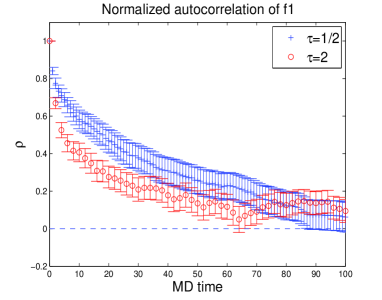
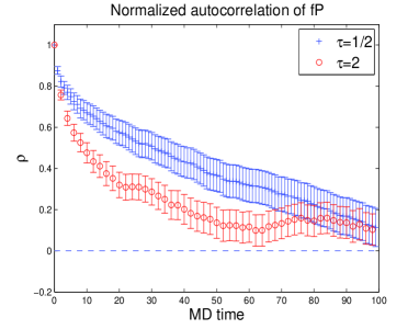
Figure 2: Autocorrelation function of the correlators $f_{1}$ and $f_{\rm P}$ (${N_{\rm f}}=2$, $\beta=5.3$, $\kappa=0.1355$, $V=24^{3}\times 32$), for different trajectory lengths.

The reduced autocorrelation times observed with long trajectories should be reflected in faster thermalization of the same observables. We thus perform the following experiment. We start from an ensemble of 16 small-volume and small-quark mass configurations with a background chromo-electric field. The correlators $f_{P}$ and $f_{P}^{\prime}$, defined by the correlation from one or the other boundary to the middle time-slice, are thus not equal. We then change the SF boundary conditions so as to remove the background field, after which $f_{P}=f_{P}^{\prime}$ holds exactly in the new thermalized ensemble. Fig. 4 shows how fast $f_{P}-f_{P}^{\prime}$ thermalizes to zero with two different choices of trajectory length. The advantage of $\tau=2$ over $\tau=1/2$ is obvious in the early stages of thermalization.

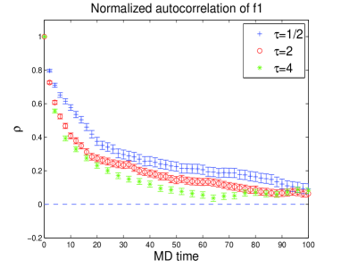
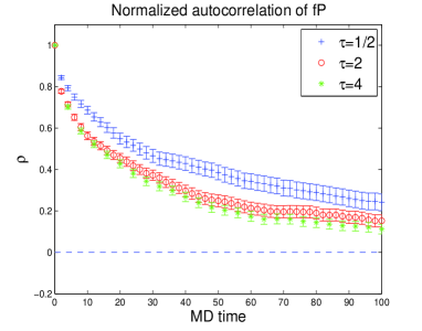
Figure 3: Autocorrelation function of the correlators $f_{1}$ and $f_{\rm P}$ in quenched QCD ($\beta=6.0$, $\kappa=0.1338$, $V=8^{3}\times 32$), for different trajectory lengths.

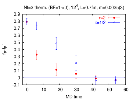
Figure 4: Thermalization of $f_{\rm P}-f_{\rm P}^{\prime}$, whose expectation value vanishes. The data points are averaged over 16 configurations taken from an ensemble where the expectation value is non-zero.

4 Conclusion

We are performing large-volume ${N_{\rm f}}=2$ simulations with O($a$) improved Wilson quarks in the Schrödinger functional at $m\simeq m_{s}/2$ to set the low-energy scale for our determination of the $\Lambda$ parameter [1] and the strange quark mass [4]. Apart from the $L/a=24$ simulations presented here, simulations at $L/a=32$ and larger $\beta$ are underway.

We have shown that the trajectory length $\tau$ is an important parameter of the Hybrid Monte-Carlo algorithm. In practice we have found that $\tau\geq 2$ is never a worse choice for long-distance observables based on fermionic correlators. The reduction in autocorrelation time is in some cases as large as a factor two. We have also provided evidence that slow-thermalization problems can be alleviated by choosing longer trajectories. For more details, as well as a discussion of stability and reversibility issues, we refer the reader to [20].

We thank Michele Della Morte, Hubert Simma, Rainer Sommer and Ulli Wolff for a stimulating collaboration and a careful reading of the manuscript. We further thank DESY/NIC for computing resources on the APE machines and the computer team for support, in particular to run on the new apeNEXT systems. This project is part of ongoing algorithmic development within the SFB Transregio 9 “Computational Particle Physics” programme.

References

- [1] M. Della Morte, R. Frezzotti, J. Heitger, J. Rolf, R. Sommer and U. Wolff [ALPHA Collaboration], Nucl. Phys. B 713 (2005) 378 [arXiv:hep-lat/0411025].
- [2] S. Sint and R. Sommer, Nucl. Phys. B 465 (1996) 71 [arXiv:hep-lat/9508012].
- [3] M. Göckeler, R. Horsley, A. C. Irving, D. Pleiter, P. E. L. Rakow, G. Schierholz and H. Stuben [QCDSF Collaboration], Phys. Lett. B 639 (2006) 307 arXiv:hep-ph/0409312.
- [4] M. Della Morte, R. Hoffmann, F. Knechtli, J. Rolf, R. Sommer, I. Wetzorke and U. Wolff [ALPHA Collaboration], Nucl. Phys. B 729 (2005) 117 [arXiv:hep-lat/0507035].
- [5] J. Gasser and H. Leutwyler, Nucl. Phys. B 250 (1985) 465.
- [6] J. Bijnens, P. Dhonte and P. Talavera, JHEP 0405, 036 (2004) [arXiv:hep-ph/0404150].
- [7] T. A. Lahde and U. G. Meissner, Phys. Rev. D 74 (2006) 034021 [arXiv:hep-ph/0606133].
- [8] M. Guagnelli, J. Heitger, R. Sommer and H. Wittig [ALPHA Collaboration], Nucl. Phys. B 560 (1999) 465 [arXiv:hep-lat/9903040].
- [9] P. de Forcrand, G. Schierholz, H. Schneider and M. Teper, Phys. Lett. B 152 (1985) 107.
- [10] K. Jansen and C. Liu, Comput. Phys. Commun. 99 (1997) 221, hep-lat/9603008.
-
[11]
M. Hasenbusch,
Phys. Lett. B 519 (2001) 177
[arXiv:hep-lat/0107019];
M. Hasenbusch and K. Jansen, Nucl. Phys. B 659 (2003) 299 [arXiv:hep-lat/0211042]. - [12] JLQCD, S. Aoki et al., Phys. Rev. D65 (2002) 094507, hep-lat/0112051.
- [13] M. Hasenbusch, PoS LAT2005 (2006) 116 [arXiv:hep-lat/0509080].
- [14] A. Ali Khan et al. [QCDSF Collaboration], Phys. Lett. B 564 (2003) 235 [arXiv:hep-lat/0303026].
- [15] C. Urbach, K. Jansen, A. Shindler and U. Wenger, Comput. Phys. Commun. 174, 87 (2006) [arXiv:hep-lat/0506011].
- [16] J. C. Sexton and D. H. Weingarten, Nucl. Phys. B 380 (1992) 665.
- [17] ALPHA collaboration, unpublished.
- [18] M. Lüscher, Comput. Phys. Commun. 165 (2005) 199 [arXiv:hep-lat/0409106].
- [19] M. Lüscher, PoS LAT2005 (2006) 002 [arXiv:hep-lat/0509152].
- [20] H. B. Meyer, H. Simma, R. Sommer, M. Della Morte, O. Witzel and U. Wolff, Comput. Phys. Commun. (in print), arXiv:hep-lat/0606004.