Nonzero chemical potential in the overlap Dirac operator and comparison to random matrix theory

Abstract:

In this talk we present the results published recently in Ref. [1], where we showed how to introduce a quark chemical potential in the overlap Dirac operator. The resulting operator satisfies a Ginsparg-Wilson relation and has exact zero modes. It is no longer $\gamma_{5}$-Hermitian, but its nonreal eigenvalues still occur in pairs. We compute the spectral density of the operator on the lattice and show that, for small eigenvalues, the data agree with analytical predictions of non-Hermitian chiral random matrix theory for both trivial and nontrivial topology. We also explain an observed change in the number of zero modes as a function of chemical potential.

Quantum chromodynamics (QCD) at nonzero baryon density is important for the study of relativistic heavy-ion collisions, neutron stars, and the early universe [2]. The effects of such a density are investigated by introducing a quark chemical potential $\mu$ in the QCD Dirac operator.

For $\mu\neq 0$ the Dirac operator loses its hermiticity properties and its spectrum moves into the complex plane. This causes a variety of problems, both analytically and numerically. Lattice simulations are the main source of nonperturbative information about QCD, but at $\mu\neq 0$ they cannot be performed by standard importance sampling methods because the measure of the functional integral, which includes the complex fermion determinant, is no longer positive definite.

A better analytical understanding of QCD at very high baryon density has been obtained by a number of methods [3], and the QCD phase diagram has been studied in model calculations based on symmetries [4]. Chiral random matrix theory (RMT) [5], which makes exact analytical predictions for the correlations of the small Dirac eigenvalues, has been extended to $\mu\neq 0$ [6], and a mechanism was identified [7] by which the chiral condensate at $\mu\neq 0$ is built up from the spectral density of the Dirac operator in the complex plane, in stark contrast to the Banks-Casher mechanism at $\mu=0$. This mechanism and its relation to the sign problem was also discussed by Splittorff in a plenary talk at this conference [8].

A first comparison of lattice data with RMT predictions at $\mu\neq 0$ was made in Ref. [9] using staggered fermions. One issue with staggered fermions is that the topology of the gauge field is only visible in the Dirac spectrum if the lattice spacing is small and various improvement and/or smearing schemes are applied [10]. To avoid these issues, we would like to work with a Dirac operator that implements a lattice version of chiral symmetry and has exact zero modes at finite lattice spacing [11]. The overlap operator [12] satisfies these requirements at $\mu=0$. In the following, we show how the overlap operator can be modified to include a nonzero quark chemical potential [1]. We then study the spectral properties of this operator as a function of $\mu$ and compare data from lattice simulations with RMT predictions. As we shall see, the overlap operator has exact zero modes also at nonzero $\mu$, which allows us, for the first time, to test predictions of non-Hermitian RMT for nontrivial topology.

We begin with the well-known definition of the Wilson Dirac operator $D_{W}$ including a chemical potential $\mu$ [15],

$$D_{W}(\mu) =\mathbbm{1}-\kappa\sum_{i=1}^{3}\left(T_{i}^{+}+T_{i}^{-}\right)-\kappa\left(e^{\mu}T_{4}^{+}+e^{-\mu}T_{4}^{-}\right)\>,$$

$$(T_{\nu}^{\pm})_{yx} =(1\pm\gamma_{\nu})U_{\pm\nu}(x)\delta_{y,x\pm\hat{\nu}}\>,$$ (1)

where $\kappa=1/(2m_{W}+8)$ with the Wilson mass $m_{W}$, the $U\in\text{SU(3)}$ are the lattice gauge fields, and the $\gamma_{\nu}$ are the usual Euclidean Dirac matrices. Unless displayed explicitly, the lattice spacing $a$ is set to unity.

The overlap operator is defined at $\mu=0$ by [12]

$$D_{\text{ov}}(0)=\mathbbm{1}+\gamma_{5}\varepsilon(\gamma_{5}D_{W}(0))\>,$$ (2)

where $\varepsilon$ is the matrix sign function and $\gamma_{5}=\gamma_{1}\gamma_{2}\gamma_{3}\gamma_{4}$. $m_{W}$ must be in the range $(-2,0)$ for $D_{\text{ov}}(0)$ to describe a single Dirac fermion in the continuum. The properties of $D_{\text{ov}}(0)$ have been studied in great detail in the past years. In particular, its eigenvalues are on a circle in the complex plane with center at $(1,0)$ and radius 1, its nonreal eigenvalues come in complex conjugate pairs, and it can have exact zero modes without fine-tuning. $D_{\text{ov}}(0)$ satisfies a Ginsparg-Wilson relation [16] of the form

$$\{D,\gamma_{5}\}=D\gamma_{5}D\>.$$ (3)

We now extend the definition of the overlap operator to $\mu\neq 0$. The operator $D_{W}(0)$ in Eq. (2) is $\gamma_{5}$-Hermitian, i.e., $\gamma_{5}D_{W}(0)\gamma_{5}=D_{W}^{\dagger}(0)$, and therefore the operator $\gamma_{5}D_{W}(0)$ in the matrix sign function is Hermitian. However, for $\mu\neq 0$, $D_{W}(\mu)$ is no longer $\gamma_{5}$-Hermitian. Defining the overlap operator at nonzero $\mu$ by

$$D_{\text{ov}}(\mu)=\mathbbm{1}+\gamma_{5}\varepsilon(\gamma_{5}D_{W}(\mu))\>,$$ (4)

we now need the sign function of a non-Hermitian matrix. In general, a function $f$ of a non-Hermitian matrix $A$ can be defined by the contour integral

$$f(A)=\frac{1}{2\pi i}\oint_{\Gamma}dz\;f(z)(z\mathbbm{1}-A)^{-1}\,,$$ (5)

where the spectrum of $A$ is enclosed by the contour $\Gamma$ and the matrix integral is defined on an element-by-element basis. A more convenient expression can be obtained if $A$ is diagonalizable. In this case we can write $A=U\Lambda U^{-1}$, where $U\in\text{Gl}(N,\mathbb{C})$ with $N=\dim(A)$ and $\Lambda=\operatorname{diag}(\lambda_{1},\ldots,\lambda_{N})$ with $\lambda_{i}\in\mathbb{C}$. Then, applying Cauchy’s theorem to Eq. (5), $f(A)=Uf(\Lambda)U^{-1}$, where $f(\Lambda)$ is a diagonal matrix with elements $f(\lambda_{i})$. In particular, the matrix sign function can be defined by [17]

$$\varepsilon(A)=U\operatorname{sign}(\operatorname{Re}\Lambda)U^{-1}\>.$$ (6)

This definition ensures that $\varepsilon^{2}(A)=\mathbbm{1}$ and gives the correct result if $\Lambda$ is real. An equivalent definition is $\varepsilon(A)=A(A^{2})^{-1/2}$ [18]. Eqs. (4) and (6) constitute our definition of $D_{\text{ov}}(\mu)$. The sign function is ill-defined if one of the $\lambda_{i}$ lies on the imaginary axis. Also, it could happen that $\gamma_{5}D_{W}(\mu)$ is not diagonalizable (one would then resort to a Jordan block decomposition). Both of these cases are only realized if one or more parameters are fine-tuned, and are unlikely to occur in realistic lattice simulations.

It is relatively straightforward to derive the following properties of $D_{\text{ov}}(\mu)$:

• It is no longer $\gamma_{5}$-Hermitian.

• It still satisfies the Ginsparg-Wilson relation (3) because of $\varepsilon^{2}(A)=\mathbbm{1}$. Thus, we still have a lattice version of chiral symmetry, and the operator has exact zero modes without fine-tuning.

• Its eigenvalues not equal to 0 or 2 no longer come in complex conjugate pairs, but every such eigenvalue $\lambda$ (with eigenvector $\psi$) comes with a partner $\lambda/(\lambda-1)$ (with eigenvector $\gamma_{5}\psi$).

• Its eigenvectors corresponding to eigenvalues 0 or 2 can be arranged to have definite chirality.

We now turn to our (quenched) lattice simulations. The computation of the sign function of a non-Hermitian matrix is very demanding. We are currently investigating various approximation schemes, but in this initial study we decided to compute the sign function and to diagonalize $D_{\text{ov}}(\mu)$ exactly using LAPACK. For the comparison with RMT we need high statistics, which restricts us to a very small lattice size. We have chosen the same parameter set as in Ref. [19] to be able to compare with previous results at $\mu=0$. The lattice size is $V=4^{4}$, the coupling in the standard Wilson action is $\beta=5.1$, the Wilson mass is $m_{W}=-2$, and the quark mass is $m_{q}=0$.

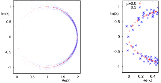
Figure 1: Spectrum of $D_{\text{ov}}(\mu)$ for $\mu=0$ and $\mu=0.3$ for a typical configuration. The figure on the right is a magnification of the region near zero.

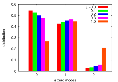
      $\mu a$ # config. 0.0 6783 0.1 8703 0.2 5760 0.3 5760 1.0 2816

Figure 2: Distribution of the number of zero mores of $D_{\text{ov}}(\mu)$ for $\mu=0,0.1,0.2,0.3,1.0$, and number of configurations (right table).

In Fig. 1 we show the spectrum of $D_{\text{ov}}(\mu)$ for a typical configuration for $\mu=0$ and $\mu=0.3$. As expected, we see that the eigenvalues move away from the circle as $\mu$ is turned on. Another observation is that the number of zero modes of $D_{\text{ov}}(\mu)$ for a given configuration can change as a function of $\mu$, see Figure 2. This can be understood from the relation between the anomaly and the index of $D_{\text{ov}}$ [20, 21],

$$-\operatorname{tr}(\gamma_{5}D_{\text{ov}})=2\operatorname{index}(D_{\text{ov}})\>,$$ (7)

which we can show to remain valid at $\mu\neq 0$. Using $\operatorname{tr}(\gamma_{5}D_{\text{ov}})=\operatorname{tr}[\varepsilon(\gamma_{5}D_{W})]$ and the fact that the eigenvalues of the sign function are $+1$ or $-1$, one has $\operatorname{index}(D_{\text{ov}})=(n_{-}^{W}-n_{+}^{W})/2$, where $n_{\pm}^{W}$ denotes the number of eigenvalues of $\gamma_{5}D_{W}(\mu)$ with real part $\gtrless 0$. Therefore the number of zero modes for a given configuration is determined by the difference of the number of eigenvalues of $\gamma_{5}D_{W}$ lying left and right of the imaginary axis. As $\mu$ changes, an eigenvalue of $\gamma_{5}D_{W}$ can move across the imaginary axis. As a result, $\operatorname{index}(D_{\text{ov}})$ changes by 1, which explains the observation. We believe that this is a lattice artefact which will disappear in the continuum limit.

         

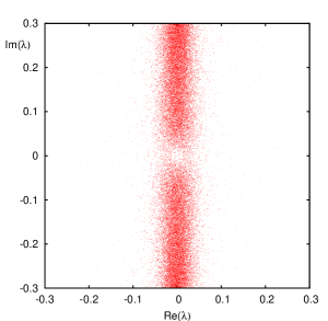
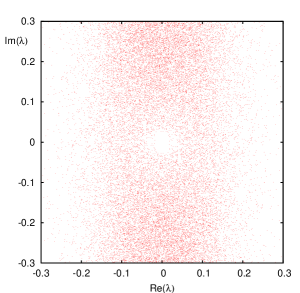
Figure 3: Scatter plot of the projected eigenvalues $\lambda$ of $D_{\text{ov}}(\mu)$ for $\mu=0.1$ (left pane) and $\mu=0.3$ (right pane). The eigenvalues are projected using $\lambda\to 2\lambda/(2-\lambda)$. At $\mu=0$ this mapping projects the eigenvalues from the GW-circle to the imaginary axis. At $\mu\neq 0$, the same mapping projects the eigenvalues onto a band parallel to the imaginary axis. As $\mu$ is increased the eigenvalues spread further into the complex plane.

The spectral density of $D_{\text{ov}}(\mu)$ is given by $\rho^{\text{ov}}(\lambda_{r},\lambda_{i})=\langle\sum_{k}\delta(\lambda-\lambda_{k})\rangle$ with $\lambda=\lambda_{r}+i\lambda_{i}$, where the average is over configurations. The distribution of (projected) eigenvalues in the complex plane is shown in Figure 3. The claim is that the distribution of the small eigenvalues of $D_{\text{ov}}(\mu)$ is universal and given by RMT. The chiral RMT model for the Dirac operator is [6]

$$D_{\text{RMT}}(\mu)=\begin{pmatrix}0&iW+\mu\\ iW^{\dagger}+\mu&0\end{pmatrix}\>,$$ (8)

where $W$ is a complex matrix of dimension $n\times(n+\nu)$ with no further symmetries (we take $\nu\geq 0$ without loss of generality). The matrix in Eq. (8) has $\nu$ eigenvalues equal to zero. The spectral correlations of $D_{\text{RMT}}(\mu)$ on the scale of the mean level spacing were computed in Refs. [22, 23, 24]. In the quenched approximation, the result for the microscopic spectral density reads

$$\rho_{s}^{\text{RMT}}(x,y)=\frac{x^{2}+y^{2}}{2\pi\alpha}e^{\frac{y^{2}-x^{2}}{4\alpha}}K_{\nu}\left(\frac{x^{2}+y^{2}}{4\alpha}\right)\int_{0}^{1}t\,dt\,e^{-2\alpha t^{2}}|I_{\nu}(tz)|^{2}\>,$$ (9)

where $z=x+iy=\lambda\Sigma V$, $I$ and $K$ are modified Bessel functions, and $\alpha=\mu^{2}f_{\pi}^{2}V$. $\Sigma$ and $f_{\pi}$ are low-energy constants that can be obtained from a two-parameter fit of the lattice data to the RMT prediction, Eq. (9). (The normalization is fixed by $\int dx\,dy\,\rho^{\text{ov}}(x,y)=12V$ and does not introduce another parameter.) For $x\ll\alpha$, Eq. (9) becomes radially symmetric [25],

$$\rho_{s}^{\text{RMT}}(x,y)\to\frac{\xi}{2\pi\alpha}K_{\nu}\left(\xi\right)I_{\nu}\left(\xi\right)$$ (10)

with $\xi=|z|^{2}/4\alpha$, and the fit only involves the single parameter $\Sigma/f_{\pi}$.

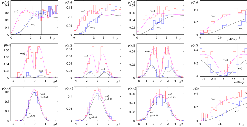
Figure 4: Density of the small eigenvalues $z=x+iy=\lambda\Sigma V$ of $D_{\text{ov}}(\mu)$ in the complex plane (after projecting $\lambda\to 2\lambda/(2-\lambda)$) for (from left to right) $\mu=0.1,0.2,0.3,1.0$. The histograms are lattice data for $\nu=0$ and $\nu=1$, and the solid lines are the corresponding RMT prediction of Eq. (9), integrated over the bin size. Top: cut along the imaginary axis, middle: cut along the real axis, bottom: cut parallel to the real axis at $y_{c}$. Vertical lines indicate the fit interval. For $\mu=1.0$ the distribution of the small eigenvalues is radially symmetric up to $|\xi|\sim 0.7$, with $\xi=|z|^{2}/4\alpha$, and therefore only the ratio $\Sigma/f_{\pi}$ can be determined from a fit to Eq. (10). In the rightmost bottom plot the data are integrated over the phase.

$\mu a$ $\Sigma a^{3}$ $f_{\pi}a$ $\Sigma a^{3}/f_{\pi}a$ $\chi^{2}/\text{dof}$ 0.0 0.0816(6) – – 1.10 0.1 0.0812(11) 0.261(6) 0.311(5) 0.67 0.2 0.0785(14) 0.245(5) 0.320(4) 0.78 0.3 0.0824(17) 0.248(5) 0.332(4) 1.03 1.0 – – 0.603(18) 0.42 Table 1: Fit results for $\Sigma$ and $f_{\pi}$. For $\mu=1.0$ only $\Sigma/f_{\pi}$ can be determined (see Figure 4).

In Fig. 4 we compare our lattice data to the RMT prediction. We display various cuts of the eigenvalue density in the complex plane as explained in the figure captions. The data agree with the RMT predictions within our statistics. $\Sigma$ and $f_{\pi}$ were obtained by a combined fit to the $\nu=0$ and $\nu=1$ data for all three cuts and are displayed in Table 1. (These numbers have no physical significance at $\beta=5.1$.)

In summary, we have shown how to include a quark chemical potential in the overlap operator. The operator still satisfies a Ginsparg-Wilson relation and has exact zero modes. The distribution of its small eigenvalues agrees with predictions of non-Hermitian RMT for trivial and nontrivial topology. Our initial lattice study should be extended to weaker coupling, larger lattices, and better statistics. Work on approximation methods to enable such studies is in progress. For small volumes, reweighting with the fermion determinant should allow us to test RMT predictions for the unquenched theory [26].

This work was supported in part by DFG. The simulations were performed on a QCDOC machine in Regensburg using USQCD software and Chroma [27], and GotoBLAS optimized for QCDOC.

References

- [1] J. Bloch and T. Wettig, Phys. Rev. Lett. 97 (2006) 012003
- [2] for a review, see O. Philipsen, PoS LAT2005 (2005) 016
- [3] for a recent review, see M.G. Alford, Nucl. Phys. (Proc. Suppl.) 117 (2003) 65 and references therein
- [4] M.A. Halasz et al., Phys. Rev. D 58 (1998) 096007
- [5] E.V. Shuryak and J.J.M. Verbaarschot, Nucl. Phys. A 560 (1993) 306; J.J.M. Verbaarschot, Phys. Rev. Lett. 72 (1994) 2531
- [6] M.A. Stephanov, Phys. Rev. Lett. 76 (1996) 4472
- [7] J.C. Osborn, K. Splittorff, and J.J.M. Verbaarschot, Phys. Rev. Lett. 94 (2005) 202001
- [8] K. Splittorff, PoS LAT2006 (2006) 023
- [9] G. Akemann and T. Wettig, Phys. Rev. Lett. 92 (2004) 102002, Erratum ibid. 96 (2006) 029902
- [10] F. Farchioni, I. Hip, and C.B. Lang, Phys. Lett. B 471 (1999) 58; E. Follana, A. Hart, and C.T.H. Davies, Phys. Rev. Lett. 93 (2004) 241601; S. Dürr, C. Hoelbling, and U. Wenger, Phys. Rev. D 70 (2004) 094502; K.Y. Wong and R.M. Woloshyn, Phys. Rev. D 71 (2005) 094508; E. Follana et al., Phys. Rev. D 72 (2005) 054501
- [11] for a review, see P. Hasenfratz, hep-lat/0406033
- [12] R. Narayanan and H. Neuberger, Nucl. Phys. B 443 (1995) 305; H. Neuberger, Phys. Lett. B 417 (1998) 141
- [13] W. Bietenholz and U.-J. Wiese, Phys. Lett. B 426 (1998) 114
- [14] W. Bietenholz and I. Hip, Nucl. Phys. B 570 (2000) 423
- [15] P. Hasenfratz and F. Karsch, Phys. Lett. B 125 (1983) 308; J.B. Kogut et al., Nucl. Phys. B 225 (1983) 93
- [16] P.H. Ginsparg and K.G. Wilson, Phys. Rev. D 25 (1982) 2649
- [17] J.D. Roberts, Int. J. Control 32 (1980) 677
- [18] N.J. Higham, Linear Algebra Appl. 212-213 (1994) 3
- [19] R.G. Edwards et al., Phys. Rev. Lett. 82 (1999) 4188
- [20] R. Narayanan and H. Neuberger, Nucl. Phys. B 412 (1994) 574
- [21] P. Hasenfratz, V. Laliena, and F. Niedermayer, Phys. Lett. B 427 (1998) 125; M. Lüscher, Phys. Lett. B 428 (1998) 342
- [22] K. Splittorff and J.J.M. Verbaarschot, Nucl. Phys. B 683 (2004) 467
- [23] J.C. Osborn, Phys. Rev. Lett. 93 (2004) 222001
- [24] G. Akemann, J.C. Osborn, K. Splittorff, and J.J.M. Verbaarschot, Nucl. Phys. B 712 (2005) 287
- [25] Eq. (479) in J.J.M. Verbaarschot, hep-th/0410211
- [26] G. Akemann and E. Bittner, Phys. Rev. Lett. 96 (2006) 222002
- [27] R.G. Edwards and B. Joó, Nucl. Phys (Proc. Suppl.) 140 (2005) 832