Phase-diagram of two-color lattice QCD in the chiral limit

Abstract

We study thermodynamics of strongly coupled lattice QCD with two colors of massless staggered fermions as a function of the baryon chemical potential $\mu$ in $3+1$ dimensions using a new cluster algorithm. We find evidence that the model undergoes a weak first order phase transition at $\mu=0$ which becomes second order at a finite $\mu$. Symmetry considerations suggest that the universality class of these phase transitions should be governed by a $O(N)\times O(2)$ field theory with collinear order, with $N=3$ at $\mu=0$ and $N=2$ at $\mu\neq 0$. The universality class of the second order phase transition at $\mu\neq 0$ appears to be governed by the decoupled $XY$ fixed point present in the $O(2)\times O(2)$ field theory. Finally we show that the quantum ($T=0$) phase transition as a function of $\mu$ is a second order mean field transition.

I INTRODUCTION

Understanding the phase diagram of Quantum Chromodynamics (QCD), as a function of temperature $(T)$ and baryon chemical potential $(\mu)$ is of great interest in the phenomenology of strongly interacting dense matter Rajagopal:2000wf . There are many excellent reviews on the subject and some recent ones can be found in Schafer:2003vz ; Rischke:2003mt ; Alford:2003eg ; Stephanov:2004wx . The only first principles approach to the subject is based on the lattice formulation of QCD in which one computes quantities using the Monte Carlo method. Unfortunately, due to a variety of algorithmic difficulties this has been difficult to accomplish. At intermediate and large chemical potentials and small temperatures the numerical methods suffer from a severe sign problem. Thus, the most reliable lattice calculations can only be found at small $\mu$ where reasonable algorithms are available deForcrand:2004bk ; Lombardo:2004uy . However, even these calculations become difficult especially for large lattices and realistic quark masses. Thus, it is fair to say that quantitatively many features of the $T-\mu$ phase diagram of QCD still remains unclear. A recent review of the status of lattice calculations at finite temperature and density can be found in Allton:2005tk ; Philipsen:2005mj .

Given the difficulties of studying the phase diagram of QCD, it is interesting to consider QCD-like theories which do not suffer from sign problems at $\mu\neq 0$ Kogut:2000ek . The sign problem is avoided due to special properties of the fermion action which makes the fermion determinant real and positive. As a price, baryons turn out to be bosons. In spite of this difference QCD-like theories provide interesting toy models for QCD. In certain cases they are also interesting in their own right. A famous example is two-color QCD and has been extensively studied over the years both theoretically Kogut:1999iv ; Wirstam:1999ds ; Ratti:2004ra ; Lenaghan:2001sd and numerically Kogut:1985un ; Kogut:1987ev ; Kaczmarek:1998wr ; Hands:1999md ; Hands:2000ei ; Kogut:2001na ; Kogut:2003ju ; Skullerud:2003yc . Two-color lattice QCD with staggered fermions (2CLQCD) is especially interesting due to an enhanced $U(2)$ symmetry at zero quark mass and baryon chemical potential. As we will see later, the long distance physics of this theory in the $T-\mu$ plane is described by an $O(N)\times O(2)$ ($N=3$ when $\mu=0$ and $N=2$ when $\mu\neq 0$) field theory. Such field theories arise naturally in many condensed matter systems Kawamura88 including the studies of spin and charge ordering in cuprate superconductors Zha02 and superfluid transitions in ³He Jones76 . More concretely, the normal-to-planar superfluid phase transition in ${}^{3}He$ is governed by an $O(3)\times O(2)$ field theory Prato , which is similar to the one that arises in 2CLQCD at $\mu=0$. Although some progress has been made in uncovering important qualitative features of the phase diagram of 2CLQCD, many quantitative questions remain: (1) What is the order of the finite temperature chiral transition at zero and non-zero chemical potentials? (2) Can the low energy physics at small $T$ and $\mu$ be understood quantitatively by an appropriate chiral perturbation theory Kogut:2003ju ? (3) What is the order of the phase transition that occurs when the lattice gets saturated with baryons at $T=0$? The reason for the lack of quantitative progress can be traced to the fact that the difficulty of calculations are similar to those in QCD at zero chemical potential. Hence, all previous studies have been limited to small lattice sizes and relatively large quark masses. Further, diquark condensation occurs in 2CLQCD and is difficult to study in the conventional approach. One usually has to add a diquark source term and then extrapolate it to zero.

Fortunately, new Monte Carlo algorithms have emerged for lattice gauge theories in the limit of infinite gauge coupling Adams:2003cc where many of the conventional algorithmic problems disappear. Although this strong coupling limit has the worst lattice artifacts, the qualitative physics is expected to be preserved. Since most of the current work is being done at couplings which can be considered rather strong, the phase diagram at these couplings may not be altered significantly as compared to the infinite coupling theory. On the other hand, thanks to the new algorithms, one can study the chiral limit on large lattices with ease at infinite coupling. Thus, studying strong coupling 2CLQCD should be a useful step in our general understanding of the subject. The strong coupling limit attracted the attention of physicists in the eighties when a variety of qualitative results were obtained using mean field theory and numerical work Blairon:1980pk ; Kawamoto:1981hw ; Kluberg-Stern:1982bs ; Martin:1982tb ; Rossi:1984cv ; Wolff:1984we ; Dagotto:1986ms ; Dagotto:1986gw ; Dagotto:1986xt ; Karsch:1988zx ; Klatke:1989xy ; Boyd:1991fb . Interestingly, even today many qualitative questions continue to addressed in this limit Bringoltz:2002qc ; Bringoltz:2003jf ; Bringoltz:2005az . The strong coupling limit of 2CLQCD was originally considered in Dagotto:1986gw ; Dagotto:1986xt ; Klatke:1989xy and has been recently reviewed in Nishida:2003uj . However, many interesting questions, including the ones raised above, have remained unanswered even in this simplified limit.

In this article we extend the directed path algorithm invented in Adams:2003cc to study strong coupling 2CLQCD in the chiral limit and attempt to answer many questions including those raised above. Our article is organized as follows. In section II we discuss the model and the expected physics in detail. In section III we explain the new algorithm which is followed by a section in which we discuss the observables and how we measure them. Section V contains our results which is followed by a section where we present a summary of our work along with conclusions. A preliminary version of this work appeared in a recent conference proceedings Chandrasekharan:2005dn .

II THE MODEL

The action of 2CLQCD we study is given by

$$S=-\sum_{x,\alpha}r_{\alpha}\eta_{\alpha}(x)\Bigg{[}e^{\mu a_{t}\delta_{t,\alpha}}\overline{\chi}(x)U_{\alpha}(x)\chi(x+\hat{\alpha})-e^{-\mu a_{t}\delta_{t,\alpha}}\overline{\chi}(x+\hat{\alpha})U_{\alpha}^{\dagger}(x)\chi(x)\Bigg{]}.$$ (1)

The Grassmann valued quark fields $\overline{\chi}(x)$ and $\chi(x)$, associated to the $3+1$ dimensional lattice site $x$ with coordinates $(x_{t},x_{1},x_{2},x_{3})$, represent row and column vectors with $2$ color components. The components will be denoted as $\overline{\chi}_{a}$ and $\chi_{a},a=1,2$. The gauge fields $U_{\alpha}(x)$ are elements of $SU(2)$ group and live on the links between $x$ and $x+\hat{\alpha}$ where $\alpha=t,1,2,3$. The factor $r_{\alpha}=1$ for $\alpha=1,2,3$ and $r_{t}=1/a_{t}$. At weak couplings $a_{t}$ acts as the temporal lattice spacing (assuming spatial lattice spacing is $1$). However there is no reason to expect this interpretation to hold at strong couplings. Thus, we think of $a_{t}$ as merely an asymmetry factor between spatial and temporal directions. It allows us to study the effects of temperature on asymmetric lattices and was already used for this purpose in Boyd:1991fb . In the dimer-baryon loop representation which we will construct later, the parameter ${1/(a_{t})^{2}}$ is more natural. By choosing an $L_{t}\times L^{d}$ lattice (periodic in all directions) we can study thermodynamics in the $L\rightarrow\infty$ limit at a fixed $L_{t}$ by defining $T=1/(a_{t})^{2}$ as the parameter that represents the temperature. Zero temperature studies involve the limit $L_{t}\rightarrow\infty$ with fixed $T$. The parameter $\mu$ represents the baryon chemical potential. The absence of the gauge action shows that we are in the strong gauge coupling limit.

II.1 Internal Symmetries

A detailed discussion of the symmetries of 2CLQCD can be found in Hands:1999md ; Nishida:2003uj . For completeness we review them briefly here. We first rewrite eq. (1) as

$$S=-\sum_{x\>{\rm even},\alpha=1,2,3}\eta_{\alpha}(x)\Bigg{[}\overline{X_{e}}(x)U_{\alpha}(x)X_{o}(x+\hat{\alpha})-\overline{X_{e}}(x)U_{\alpha}^{\dagger}(x-\hat{\alpha})X_{o}(x-\hat{\alpha})\Bigg{]}$$

$$-\sum_{x\>{\rm even}}\frac{\eta_{t}(x)}{a_{t}}\Bigg{[}\overline{X_{e}}(x)\mathrm{e}^{a_{t}\mu\sigma_{3}}U_{t}(x)X_{o}(x+\hat{t})-\overline{X_{e}}(x)\mathrm{e}^{-a_{t}\mu\sigma_{3}}U_{t}^{\dagger}(x-\hat{t})X_{o}(x-\hat{t})\Bigg{]}$$

(2)

where $\overline{X_{e}}$ and $X_{o}$ are given by

$$\overline{X_{e}}=(\bar{\chi}_{e},-\chi_{e}^{tr}\tau_{2}),\quad\quad X_{o}=\left(\begin{array}[]{c}\chi_{o}\cr-\tau_{2}\bar{\chi}_{o}^{tr}\end{array}\right)$$ (3)

In our notation $\vec{\sigma}$ are Pauli matrices that mix $\chi$ and $\overline{\chi}^{tr}$ present in $X_{o}$ and $\overline{X}_{e}$ while $\vec{\tau}$ are Pauli matrices that act on the color space. Thus, $\tau_{2}U\tau_{2}=U^{\star}$ since $U$ is an element of $SU(2)$.

Clearly, when $\mu=0$ our model has a $U(2)$ global symmetry:

$$X_{o}\rightarrow VX_{o},\quad\overline{X}_{e}\rightarrow\overline{X}_{e}V^{\dagger},\qquad V=\exp(i\vec{\alpha}\cdot\vec{\sigma}+i\phi)\in U(2).$$ (4)

This symmetry is reduced to $U_{B}(1)\times U_{C}(1)$ in the presence of a chemical potential:

$$\begin{array}[]{ll}U_{B}(1):&\quad\quad X_{o}\rightarrow\exp(i\sigma_{3}\phi)X_{o},\quad\overline{X}_{e}\rightarrow\overline{X}_{e}\exp(-i\sigma_{3}\phi)\cr U_{C}(1):&\quad\quad X_{o}\rightarrow\exp(i\phi)X_{o},\quad\overline{X}_{e}\rightarrow\overline{X}_{e}\exp(-i\phi).\end{array}$$ (5)

Here $U_{B}(1)$ is the baryon number symmetry $\chi(x)\rightarrow\mathrm{e}^{i\phi}\chi(x),\quad\overline{\chi}(x)\rightarrow\overline{\chi}(x)\mathrm{e}^{-i\phi}$ and $U_{C}(1)$ is the chiral symmetry of staggered fermions $\chi(x)\rightarrow\mathrm{e}^{i\phi\varepsilon(x)}\chi(x)$, $\overline{\chi}(x)\rightarrow\overline{\chi}(x)\mathrm{e}^{i\phi\varepsilon(x)}$ where $\varepsilon(x)=(-1)^{x_{t}+x_{1}+x_{2}+x_{3}}$.

II.2 Properties of the Ground State

When $\mu=0$ one expects the chiral condensate, which is not invariant under the $U(2)$ symmetry, to get a non-zero vacuum expectation value. Note that

$$\hat{\Phi}_{i}(x)=\left\{\begin{array}[]{cc}\frac{-i}{2}X_{o}^{T}\sigma_{2}[\sigma_{i}\otimes\tau_{2}]X_{o}&x\in\mbox{odd}\cr\frac{i}{2}\bar{X}_{e}[\sigma_{i}\otimes\tau_{2}]\sigma_{2}\bar{X}_{e}^{T}&x\in\mbox{even}\end{array}\right.\ \ i=1,2,3$$ (6)

transform as components of a three vector under the $SU(2)$ subgroup of the $U(2)$ symmetry group. It is easy to check that

$$\hat{\Phi}_{1}=i[\chi_{1}\chi_{2}+\bar{\chi_{1}}\bar{\chi}_{2}],\hat{\Phi}_{2}=[-\chi_{1}\chi_{2}+\bar{\chi_{1}}\bar{\chi}_{2}],\hat{\Phi}_{3}=\bar{\chi}\chi=[\bar{\chi_{1}}\chi_{1}+\bar{\chi}_{2}\chi_{2}],$$ (7)

Thus, the chiral condensate is the third component of a complex three vector. In addition all the components carry the same non-zero $U_{C}(1)$ chiral charge.

The above discussion makes it clear that the chiral condensate being non-zero is just a matter of choice. More generally, the ground state of the theory is such that $\langle\Phi_{i}\rangle=(\hat{n})_{i}\mathrm{e}^{i\theta}$, where $\hat{n}$ is some constant unit three vector. With this choice, the ground state still remains invariant under a $U(1)$ subgroup given by $V=\exp(i\theta\ \hat{n}\cdot\vec{\sigma})$ which implies that the $U(2)$ symmetry is broken to a $U(1)$ subgroup (note that the $U(1)$ subgroup must be a part of the $SU(2)$ subgroup of $U(2)$). When one says that the chiral condensate is non-zero, one implicitly chooses $\hat{n}$ along the third direction. This then implies $\langle\Phi_{1}\rangle=\langle\Phi_{2}\rangle=0$. However when we study the effects of the chemical potential, it is natural to pick the ground state such that $\langle\Phi_{2}\rangle\neq 0$ and $\langle\Phi_{1}\rangle=\langle\Phi_{3}\rangle=0$ which implies that the diquark condensate, $\langle\chi_{1}\chi_{2}\rangle=\langle\bar{\chi}_{2}\bar{\chi}_{1}\rangle\neq 0$ while the chiral condensate vanishes. Note that even though $\langle\bar{\chi}\chi\rangle=0$ the theory still breaks the $U_{C}(1)$ symmetry since the diquark condensates carry a chiral charge.

When $\mu\neq 0$ the $U(2)$ global symmetry is explicitly broken to $U_{B}(1)\times U_{C}(1)$. At small $\mu$ both the $U(1)$ symmetries are expected to break spontaneously since the diquark condensate continues to be non-zero. As $\mu$ increases the density of baryons increases and at a critical value $\mu_{c}$ the lattice becomes saturated with baryons which means that for $\mu\geq\mu_{c}$ the diquark condensate vanishes. If this phase transition is second order, the low energy physics close to $\mu_{c}$ will be governed by a non-relativistic field theory. Renormalization group arguments indicate that this field theory is governed by mean field theory in $d\geq 2$ ($d$ represents spatial dimensions) Fisher89 .

II.3 Finite temperature phase transition

At high temperatures all the symmetries are expected to be restored. This implies one must have a finite temperature phase transition for $\mu<\mu_{c}$. The order of this transition both at $\mu=0$ and $\mu\neq 0$ in not known. Since the order parameter at $\mu=0$ is a complex 3-vector, its fluctuations are governed by the Landau-Ginzburg (LG) Hamiltonian of the $3$-component complex field $\psi(x)$. The $U(2)$ symmetry is manifest as a $O(3)\times O(2)$ symmetry. Theories with $N$-component complex scalar fields with $O(N)\times O(2)$ symmetry are interesting in condensed matter physics in describing a variety of materials Kawamura88 , and are described by the action (or classical Hamiltonian),

$$S=\int d^{d}x\ \Bigg{\{}\partial_{\mu}\psi^{*}\cdot\partial_{\mu}\psi+r\psi^{*}\cdot\psi+u(\psi^{*}\cdot\psi)^{2}+v|\psi\cdot\psi|^{2}\Bigg{\}}.$$ (8)

When $r<0$, depending on the sign of $v$, two classes of ground states are allowed (note $u>0$ is necessary for stability). When $v>0$ the ground state has a spiral or helical order, while when $v<0$ the ground state has collinear or sinusoidal order. Since we found that $\psi_{i}\equiv\langle\Phi_{i}\rangle=\hat{n}_{i}\mathrm{e}^{i\theta}$, we discover that close to the finite temperature phase transition the long distance physics of 2CLQCD with massless staggered fermions at $\mu=0$ is described by the above complex field theory with $N=3$ and collinear order ($v<0$). This field theory is of interest in the study of the normal-to-planar superfluid transition in ³He Prato . The question of whether the $N=3$ theory with collinear order can be second order still remains unresolved. While the $\epsilon$-expansion predicts a fluctuation driven first order transition Kawamura88 recent results claim that a second order fixed point indeed exists Prato . As we will see later, in our work we find a weak first order transition.

It is easy to argue that in the presence of the baryon chemical potential the finite temperature phase transition must be governed by a Landau-Ginsburg Hamiltonian similar to the one above but with $N=2$. Note that the symmetry in the microscopic theory is reduced to $U(1)\times U(1)$ which is manifest in the LG theory as an $O(2)\times O(2)$ symmetry. Further, near a finite temperature phase transition the presence of a chemical potential does not usually break charge conjugation symmetries in the low energy effective theory. For $N=2$ it is possible to define new fields

$$\left(\begin{array}[]{c}\varphi_{1}\cr\varphi_{2}\end{array}\right)=\frac{1}{\sqrt{2}}\left(\begin{array}[]{cc}1&i\cr i&1\end{array}\right)\quad\left(\begin{array}[]{c}\psi_{1}\cr\psi_{2}\end{array}\right),$$ (9)

such that the LG Hamiltonian becomes

$$S = \int d^{d}x\ \Bigg{\{}\Bigg{[}\sum_{i=1}^{2}\Big{(}|\partial_{\mu}\varphi_{i}|^{2}+r|\varphi_{i}|^{2}+u|\varphi_{i}|^{4}\Big{)}\Bigg{]}+2(u+2v)|\varphi_{1}|^{2}|\varphi_{2}|^{2}\Bigg{\}}$$ (10)

It is then obvious that when $v<0$ there is always a decoupled $XY$ fixed point at $(u+2v)=0$ Bak76 . Using the knowledge of the critical exponents in the $XY$ model it can be established that this decoupled fixed point is stable Aha76 ; Pel02 . However, the flow to this fixed point is rather slow so that corrections to the $XY$ scaling can be substantial until one is very close to the critical point Vicari . At a non-zero value of $\mu$ we indeed find a second order transition. A naive analysis indicates that the critical exponents are different from the $XY$ exponents, however when the expected corrections to scaling are included the $XY$ exponents can be used to fit our data.

III Dimer-Baryonloop Model

III.1 Dimer-Baryonloop Configurations

One of the computational advantages of the strong coupling limit is that in this limit it is possible to rewrite the partition function,

$$Z=\int[DU][d\overline{\chi}d\chi]\exp(-S),$$ (11)

as a sum over configuration containing gauge invariant objects, namely monomers, dimers, and baryonloops Rossi:1984cv ; Karsch:1988zx ; Dagotto:1986gw ; Klatke:1989xy . Monomers are absent in the massless theory. In the case of 2CLQCD a lattice configuration $K$ of dimers and baryonloops is constructed as follows: (1) Every link of the lattice connecting the site $x$ with the neighboring site $x+\hat{\alpha}$ contains either a dimer $k_{\alpha}(x)=0,1,2$ or a directed baryon-bond $b_{\alpha}(x)=-1,0,1$. When $k_{\alpha}(x)=0$, it means that the link does not contain a dimer, while $k_{\alpha}=1(2)$ implies that the link contains a single (double) dimer. Similarly $b_{\alpha}(x)=0$ means the link does not contain a baryon-bond, while $b_{\alpha}(x)=1$ means the baryon-bond is directed from $x$ to $x+\hat{\alpha}$ and $b_{\alpha}(x)=-1$ means it is directed from $x+\hat{\alpha}$ to $x$. We will also allow $\hat{\alpha}$ to be negative. Thus, if $\alpha$ was positive, $k_{-\alpha}(x)$ and $b_{-\alpha}(x)$ will represent dimers and baryon-bonds connecting $x$ with $x-\hat{\alpha}$. (2) If a site is connected to baryon-bonds then it must have exactly one incoming baryon-bond and one outgoing baryon-bond. Further it cannot be connected to dimers. Thus baryon-bonds always form self-avoiding closed baryonloops. (3) Every lattice site $x$ that does not contain a baryon-bond must satisfy the constraint

$$\sum_{\alpha}k_{\alpha}(x)=2$$ (12)

where the direction $\alpha$ in the sum takes negative values also. This implies that sites connected by single dimers also form a loop which we call a dimer-loop. An example of a configuration $K$ is given in Figure 1.

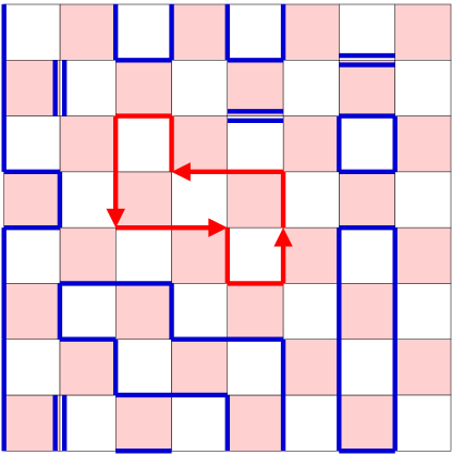
Figure 1: An example of a dimer-baryonloop configuration.

III.2 Updating Algorithms

Given the set $\{K\}$ of dimer-baryonloop configurations described above, eq. (1) can be rewritten as Klatke:1989xy ,

$$Z=\sum_{\{K\}}\quad\exp\left(\sum_{x}\Bigg{\{}\Big{(}k_{t}(x)+|b_{t}(x)|\Big{)}\log(T)+\frac{2\mu b_{t}(x)}{\sqrt{T}}\Bigg{\}}\right).$$ (13)

Since the partition function is written as a sum over positive definite terms, a Monte-Carlo algorithm can in principle be designed to the study this system. However, the algorithm needs to preserve many constrains. A method to do this was developed in Syl02 in the context of quantum spin models and later extended to dimer models in Adams:2003cc . We will now discuss an extension of these ideas to update the configurations $K$. In particular we consider three types of updates: a dimer-baryon loop flip update, a dimer update and a baryon update. Below, we discuss each of these updates in detail. Remember that we assume $k_{\alpha}(x)=k_{-\alpha}(x+\hat{\alpha})$. The dimer update and baryon updates have been described such that this redundant information also gets updated automatically.

III.2.1 Dimer-baryon loop flip update

This update is based on the observation that every baryon loop’s orientation can be flipped without violating any constraints. Further a baryonloop can be converted into a dimer-loop and vice-versa. Thus, every loop can be in one of three states: a dimer-loop or a baryonloop with two different orientations. Let $Y$ be the subset of lattice sites that are connected to either a dimer-loop or a baryonloop. $V_{Y}$ will be the number of these sites. We pick a site from $Y$ at random and change the state of the loop ${\cal C}$ connected to that site to one of the three allowed states. The change can be accomplished using a heat-bath (or similar) update if we assign the following weights to the three states: a dimer-loop carries a weight $1$ while the baryonloop (in either orientation) carries the weight $\exp[2\mu W_{t}({\cal C})]$, where

$$W_{t}({\cal C})=\sum_{x\in{\cal C}}b_{t}(x)$$ (14)

Note that $W_{t}({\cal C})$ changes sign if its orientation is flipped.

III.2.2 The Dimer Update

Let $D$ be the set of sites connected by $k_{\alpha}(x)=1,2$ and $V_{D}$ be the number of such sites. The dimer update changes the configuration on a subset of $D$. The update is as follows:

1. A lattice site $x\in D$ is selected randomly

2. If the site $x$ lies on a dimer-loop, then there will be two different directions $\hat{\alpha}$ such that $k_{\alpha}(x)=1$. One of these two directions is picked at random. Else there will be one direction $\hat{\alpha}$ such that $k_{\alpha}(x)=2$. In that case this direction is picked.

3. If the update just started and $x$ is the first site, a virtual monomer is created at $x$. If not one is added to $k_{\alpha^{\prime}}(x)$ where $\alpha^{\prime}$ is the direction from which $x$ was reached. One is subtracted from $k_{\alpha}(x)$ and the update moves to the neighboring site $y=x+\hat{\alpha}$. We will call $x$ as an “active site” and $y$ as a “passive site” in the notation of Adams:2003cc . See next subsection for more details.

4. With all the neighboring sites $y+\hat{\alpha^{\prime}}$ that belong to $D$ a non-zero weight $W_{\alpha^{\prime}}$ is associated. If $\hat{\alpha^{\prime}}$ is a temporal direction then $W_{\alpha^{\prime}}=T$, otherwise $W_{\alpha^{\prime}}=1$. If the neighboring site does not belong to $D$ then the weight is zero. For future reference we define the total dimer weight on the site $y$ as $W_{D}(y)=\sum_{\alpha^{\prime}}W_{\alpha^{\prime}}$. Now based on the weights $W_{\alpha^{\prime}}$ a heat-bath (or similar) procedure is used to pick a new direction $\hat{\alpha^{\prime}}$. One is subtracted from $k_{\alpha}(y)$ and one is added to $k_{\alpha^{\prime}}(y)$. The update then moves to the neighboring site $x=y+\hat{\alpha^{\prime}}$.

5. If the site $x$ is not the site which was picked in step 1, the update moves to step 2. Otherwise the site $x$ will contain one virtual monomer and one direction $\hat{\alpha}$ such that $k_{\alpha}(x)=1$. With probability half the direction $\hat{\alpha}$ is picked and the update moves to step 3 and with the remaining probability half the virtual monomer on the site is removed and the update ends.

III.2.3 The Baryon Update

The third update is just a minor modification of the dimer update. Let $B$ be the set of sites connected to $k_{\alpha}(x)=2$ or containing a baryonloop and $V_{B}$ the number of such sites. The baryon update changes the configuration on a subset of $B$. The update is as follows:

1. A lattice site $x$ in $B$ is selected randomly.

2. If the site $x$ lies on a baryonloop, then there will be one direction $\hat{\alpha}$ such that $b_{\alpha}(x)=-1$. This direction is picked. On the other hand if $x$ is not on a baryonloop then there will be one direction $\hat{\alpha}$ such that $k_{\alpha}(x)=2$. In that case this direction is picked.

3. If the update just started and $x$ is the first site, a virtual “diquark” is created at $x$. Otherwise, one is subtracted from $b_{\alpha^{\prime}}(x)$, where $\alpha^{\prime}$ is the direction from which $x$ was reached. If $b_{\alpha^{\prime}}(x)=0$ after the subtraction then $k_{\alpha^{\prime}}$ is set to 2. One is added to $b_{\alpha}(x)$ and if $k_{\alpha}(x)=2$ then it is set to zero. The update moves to the neighboring site $y=x+\hat{\alpha}$. We will call $x$ as an “active site” and $y$ as a “passive site” in the notation of Adams:2003cc . See next subsection for more details.

4. With all the neighboring sites $y+\hat{\alpha^{\prime}}$ that belong to $B$ a non-zero weight $W_{\alpha^{\prime}}$ is associated. If $\hat{\alpha^{\prime}}$ is the positive temporal direction then $W_{\alpha^{\prime}}=T\exp(2\mu a_{t})$, if it is along the negative temporal direction then $W_{\alpha^{\prime}}=T\exp(-2\mu a_{t})$, otherwise $W_{\alpha^{\prime}}=1$. If the neighboring site does not belong to $B$ then its weight is zero. For future reference we define the total baryon weight on the site $y$ as $W_{B}(y)=\sum_{\alpha^{\prime}}W_{\alpha^{\prime}}$. Now based on the weights $W_{\alpha^{\prime}}$ an over-relaxation procedure is used to pick a new direction $\hat{\alpha^{\prime}}$. One is subtracted from $b_{\alpha}(x)$ and if $k_{\alpha}(x)=2$ then $k_{\alpha}(x)$ is set to zero. One is added to $b_{\alpha^{\prime}}(x)$ and if $b_{\alpha^{\prime}}(x)=0$ after the addition then $k_{\alpha^{\prime}}(x)$ is set to two. The update then moves to the site $x=y+\hat{\alpha^{\prime}}$.

5. If the site $x$ is not the site which was picked in step 1, the update moves to step 2. Otherwise the site $x$ will contain one virtual diquark and it would have been reached from the direction $\hat{\alpha^{\prime}}$. One is subtracted from $b_{\alpha^{\prime}}(x)$ and if $b_{\alpha^{\prime}}(x)=0$ after the subtraction then $k_{\alpha^{\prime}}$ is set to 2. The virtual diquark on the site is removed and the update ends.

III.3 Active versus Passive Sites

In the definition of the dimer and baryon updates we have defined active and passive sites. The passive sites play an important role during the measurement of observables. Hence we clarify these two class of sites further. Both the dimer and baryon updates are directed loop updates. They start on a site $x$, which is called an active site. Then they go through a series of sites which are referred to as passive and active alternately. Thus the second site is a passive site, the third is an active site and so on. If the first site is such that $\varepsilon(x)=1$ then all passive sites $y$, visited during the update, have $\varepsilon(y)=-1$ and vice-versa. The weights $W_{D}(y)$ and $W_{B}(y)$ for passive sites encountered during the updates will play an special role in the measurement of correlation functions as discussed below.

III.4 Detailed Balance and Ergodicity

Each of the three updates satisfy detailed balance. The proof of detailed balance for the the dimer-baryon loop flip update is straight forward and conventional. On the other hand the proofs for the dimer and baryon updates need some understanding of directed loop algorithms. Once this is clear, the proof is essentially straight forward. We refer the reader to Adams:2003cc ; Syl02 and do not prove detailed balance of these two algorithms in this article. The combination of the three updates makes the algorithm ergodic. To see this we note that there is always possible to flip all the baryonloops into dimer-loops. Once this is done one can use the proof given in Adams:2003cc to show that dimer updates are ergodic in the space of configurations that purely consist of dimers.

IV Observables

A variety of observables can be measured with our algorithm. We will focus on the following:

• The chiral two point function is given by

  $$G_{C}(z,z^{\prime})=\Bigg{\langle}\bar{\chi}(z)\chi(z)\bar{\chi}(z^{\prime})\chi(z^{\prime})\Bigg{\rangle}$$ (15)

  and the chiral susceptibility $\chi_{C}$ is

  $$\chi_{C}\equiv\frac{1}{V}\sum_{z^{\prime}}G_{C}(z,z^{\prime})$$ (16)

  where $V=L^{3}L_{t}$. Both these observables can be measured easily during the dimer update. It is possible to show that Adams:2003cc

  $$G_{C}(z,z^{\prime})=\Bigg{\langle}\sum_{y}\frac{V_{D}\delta_{x,z}\delta_{y,z^{\prime}}}{W_{D}(y)}\Bigg{\rangle}$$ (17)

  where $x$ is the first site of the dimer update and the sum is over all the passive sites $y$ encountered during the update. $V_{D}$ and $W_{D}(y)$ were defined in the previous section.

• The diquark two point function is given by

  $$G_{B}(z,z^{\prime})=\Bigg{\langle}\chi_{1}(z)\chi_{2}(z)\bar{\chi}_{2}(z^{\prime})\bar{\chi}_{1}(z^{\prime})\Bigg{\rangle}$$ (18)

  and the diquark susceptibility $\chi_{B}$ is given by

  $$\chi_{B}\equiv\frac{1}{V}\sum_{z^{\prime}}G_{B}(z,z^{\prime})$$ (19)

  These can be computed during the baryon update by using

  $$G_{B}(z,z^{\prime})=\Bigg{\langle}\sum_{y}\frac{V_{B}\delta_{x,z}\delta_{y,z^{\prime}}}{W_{B}(y)}\Bigg{\rangle}$$ (20)

  where $x$ is the first site picked during the update and the sum is over all the passive sites $y$ encountered during the baryon update. $V_{B}$ and $W_{B}(y)$ were defined in the previous section.

• Baryon density $n_{B}$ is defined as

  $$n_{B}\equiv\frac{1}{2V}\frac{\partial\ln Z}{\partial\mu}$$ (21)

  and in the dimer-baryon loop flip update it can be measured by the formula

  $$n_{B}=\Bigg{\langle}\frac{V_{Y}}{V}\frac{W_{t}({\cal C})}{S({\cal C})}\frac{\sinh(2\mu W_{t}({\cal C}))}{1+2\cosh(2\mu W_{t}({\cal C}))}\Bigg{\rangle}$$ (22)

  where ${\cal C}$ is the dimer-baryon loop picked, $V_{Y}/V$ is the fraction of the lattice sites that contain dimer-baryon loops, $S({\cal C})$ is the size of the loop and $W_{t}({\cal C})$(defined earlier) is the temporal winding of the baryon loop.

• The helicity modulus associated with the $U(1)$ chiral symmetry $Y_{C}$

  $$Y_{C}\equiv\frac{1}{3V_{s}}\sum_{\mu=1,2,3}\Bigg{\langle}\Bigg{(}\sum_{x}A_{\mu}(x)\Bigg{)}^{2}\Bigg{\rangle}$$ (23)

  where

  $$A_{\mu}(x)=\varepsilon(x)\Big{(}|b_{\mu}(x)|+k_{\mu}(x)\Big{)}$$ (24)

  and $V_{s}=L^{3}$.

• The helicity modulus associated with the $U(1)$ baryon number symmetry $Y_{B}$

  $$Y_{B}\equiv\frac{1}{3V_{s}}\sum_{\mu=1,2,3}\Bigg{\langle}\Bigg{(}\sum_{x}B_{\mu}(x)\Bigg{)}^{2}\Bigg{\rangle}$$ (25)

  where

  $$B_{\mu}(x)=\left[b_{\mu}(x)\right]$$ (26)

Both $Y_{C}$ and $Y_{B}$ are observables that can be calculated easily for each configuration $K$ and averaged. Note also that our definitions of $Y_{C}$ and $Y_{B}$ are natural at finite temperatures.

V Results

V.1 Zero Chemical Potential

In a finite volume there is no spontaneous symmetry breaking. However, the effects of symmetry breaking can still be studied by examining the large volume limit of $\chi_{C}$ and $\chi_{B}$; if the symmetry is broken in the infinite volume limit, we expect these susceptibilities to grow with the volume of the system. From symmetry considerations at $\mu=0$ it is possible to show that $G_{C}(z,z^{\prime})=2G_{B}(z,z^{\prime})$ which implies $\chi_{C}=2\chi_{B}$. Symmetry breaking can also be observed through the helicity modulus $Y_{C}$ and $Y_{B}$; both must reach a non-zero constant if the symmetry breaking pattern is as expected. All these can be understood quantitatively using the low energy effective action

$$S_{\rm eff}=\int d^{d}x\ \Big{\{}\frac{B^{2}}{2}(\partial_{\mu}\vec{S})\cdot(\partial_{\mu}\vec{S})+\frac{F^{2}}{2}(\partial_{\mu}\vec{u})\cdot(\partial_{\mu}\vec{u})\Big{\}}$$ (27)

where $\vec{S}(x)$ and $\vec{u}(x)$ are unit three and two vector fields respectively. Finite size scaling formula for various quantities can be obtained following the discussion in Hasenfratz:1989pk . We note that this approach to low energy physics is equivalent to others found in the literature Kogut:1999iv ; Kogut:2000ek ; Kogut:2003ju .

At a fixed value of $L_{t}$ the parameter $T$ can be increased to induce a phase transition between a low temperature phase with spontaneous symmetry breaking and a high temperature symmetric phase. In order to study this phase transition we have performed extensive calculations at a fixed $L_{t}=4$ for different spatial lattice sizes $L$ varying from $16$ to $256$ and for many different values of $T$. The low energy effective theory introduced in eq. (27) with $d=3$ can then be used to predict the signatures of the broken phase. We have studied two such signatures: (1) $Y_{C}$ and $Y_{B}$ go to non-zero constants at large $L$. Extending the calculations of Hasenfratz:1989pk one can show Error

$$Y_{C}=F^{2}+\frac{b}{L}+\frac{c}{L^{2}}+...;\qquad Y_{B}=\frac{2B^{2}}{3}+\frac{b^{\prime}}{L}+\frac{c^{\prime}}{L^{2}}+....$$ (28)

(2) The finite size scaling of the chiral susceptibility is given by Error

$$\chi_{C}=\frac{\Sigma^{2}}{6}\Big{\{}L^{3}+\beta_{1}(\frac{2}{B^{2}}+\frac{1}{F^{2}})L^{2}\Big{\}}+aL$$ (29)

where $\beta_{1}=0.226$ is the shape coefficient for cubic boxes Hasenfratz:1989pk and $\Sigma/\sqrt{L_{t}}=\langle\overline{\chi}\chi\rangle$. Figure 2 gives our results at $T=2.918$ which is a value of $T$ in the broken phase. The graph shows that the above expectations are satisfied well.

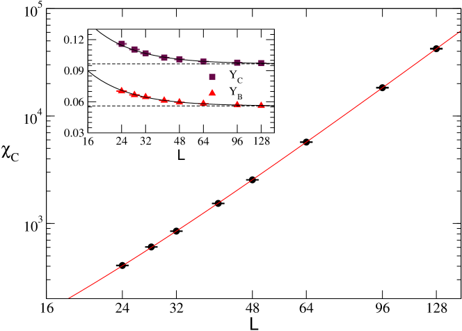
Figure 2: The inset shows the data for $Y_{C}$ and $Y_{B}$ as a function of $L$. The lines shown are fits to eq. (28) which yields $F^{2}=0.0965(5)$ and $B^{2}=0.0839(6)$. The main figure shows the plot of $\chi_{C}$ versus $L$ for $T=2.918$. The solid line is a fit to eq. (29) with $F^{2}$ and $B^{2}$ fixed to the values quoted above. The fit yields $\Sigma=0.3364(7)$ and $a=2.6(1)$ with a $\chi^{2}/DOF=0.5$.

Figure 3 shows the dependence of $\chi_{C}$ as a function of $L$ for different temperatures. Using the data for $L\leq 256$ we find that $\chi_{C}$ increases as $L^{3}$ for $T\leq 2.9275$, but saturates for $T\geq 2.9285$ as $L$ becomes large. Thus, we think $T_{c}$ is between these two temperatures. For a second order transition, close to $T_{c}$, one expects

$$\chi_{C}L^{\eta-2} = [g_{0}+g_{1}(T/T_{c}-1)L^{1/\nu}+...],$$ (30a)

$$Y_{C}L = [f_{0}+f_{1}(T/T_{c}-1)L^{1/\nu}+....],$$ (30b)

which was recently observed in other strong coupling theories Chandrasekharan:2003im ; Chandrasekharan:2003qv ; Chandrasekharan:2004uw . Our data does not fit well to this form. Clearly, the data for $\chi_{C}$ shows more structure than can be captured by the above relations. We have also verified that $Y_{C}L$ does not seem to scale as a constant for large $L$ anywhere in the range $T=2.928\pm 0.002$. Hence we think that the transition is not second order. Interestingly, we are able to fit the non-monotonic behavior in $\chi_{C}$ at $T=2.9285$ and $2.9292$ using the relation

$$\chi_{C}=\frac{\tilde{a}+\tilde{b}L^{3}\exp(-\Delta{\cal F}L^{3})}{1+\tilde{c}\exp(-\Delta{\cal F}L^{3})}$$ (31)

as long as we use data for $L\geq 48$. This form is natural in the presence of two phases (one broken and one symmetric) whose free energy densities differ by $\Delta{\cal F}$. This leads us to conclude that the phase transition is indeed first order.

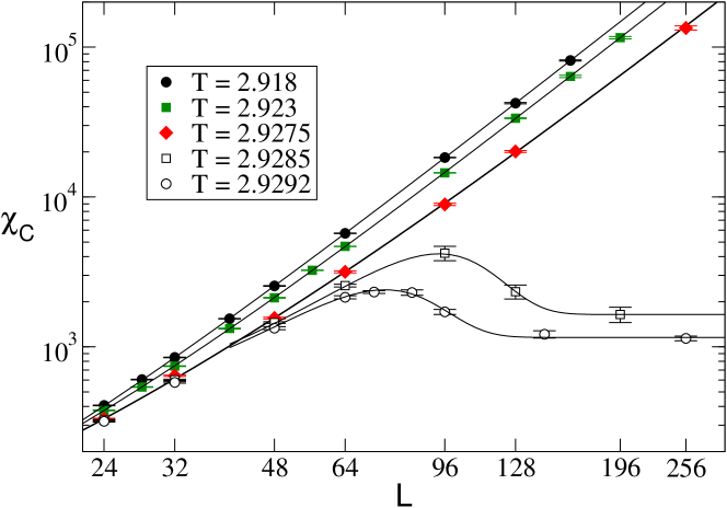
Figure 3: This figure shows the plot of $\chi_{C}$ versus $L$ for different values of $T$ across the phase transition. The solid lines for $T\leq 2.9275$ are fits to eq. (29) while those for $T=2.9285$ and $T=2.9292$ are fits to eq. (31). We find $\tilde{a}=1650(200),1150(50)$, $\tilde{b}=0.030(5),0.027(4)$, $\tilde{c}=2.5(5),2.0(4)$ and $\Delta F=2\times 10^{-6},4\times 10^{-6}$ for the two temperatures. All the fits have $\chi^{2}/DOF$ less than $1$.

The existence of a first order transition implies that the correlation lengths at the critical point do not diverge. In that case how big are these lengths at the transition? In the high temperature phase one can compute screening masses $M_{\pi}$, $M_{B}$ from the exponential decay of $G_{c}(z,z^{\prime})$ and $G_{B}(z,z^{\prime})$ respectively, for large spatial separations between $z$ and $z^{\prime}$. At $\mu=0$ we expect $M_{\pi}=M_{B}$. In the broken phase $F^{2}$ and $B^{2}$ have dimensions of mass and are the relevant physical scales in the problem. In figure 4 we show the behavior of $M_{B}$, $F^{2}$ and $B^{2}$ which have been obtained after extrapolations to infinite volumes. As can be seen, the correlation lengths close to the transition are extremely large, about $40-50$ lattice units, indicating that the transition is a weak order transition. If the transition was second order, we would have expected $F^{2}=a_{0}(T_{c}-T)^{\nu}$, $B^{2}=b_{0}(T_{c}-T)^{\nu}$ and $M_{B}=c_{0}(T-T_{c})^{\nu}$. Interestingly, these relations describe the data reasonably well, but with different $T_{c}$ and $\nu$ in the two phases. In the low temperature phase a combined fit of $F^{2}$ and $B^{2}$ gives $a_{0}=0.562(3)$, $b_{0}=0.488(3)$, $T_{c}=2.92856(4)$ and $\nu=0.387(2)$ with a $\chi^{2}/DOF=1.5$. On the other hand the fit of $M_{B}$ gives $c_{0}=0.64(5)$, $T_{c}=2.9266(6)$ and $\nu=0.50(3)$ with a $\chi^{2}/DOF=2.2$. A combined fit of all the data on both sides of the transition with a single $T_{c}$ and $\nu$ does not fit well confirming our claim that the transition is first order.

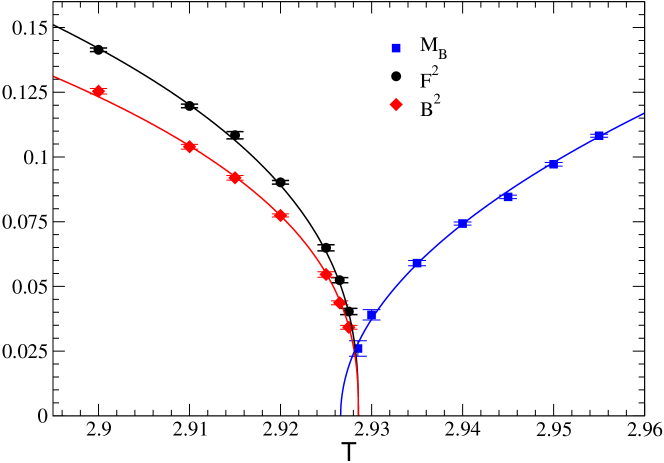
Figure 4: This figure shows the plot of $M_{B}$, $F^{2}$ and $B^{2}$ as a function of $T$. The solid lines are fits to the data as discussed in the text.

V.2 Non-zero Chemical Potential

Having established a first order transition at zero chemical potential we next focus on the finite temperature transition at $\mu=0.3$ with $L_{t}=4$. The chemical potential reduces the symmetry of the theory to $U_{B}(1)\times U_{C}(1)$. At low temperatures both the $U(1)$ symmetries are broken leading to two Goldstone bosons. The two correlators $G_{C}(z,z^{\prime})$ and $G_{B}(z,z^{\prime})$ are no longer related: $G_{c}(z,z^{\prime})$ decays exponentially while $G_{B}(z,z^{\prime})$ remains non-zero for large $|z-z^{\prime}|$. This means $\chi_{C}$ saturates for large $L$ while $\chi_{B}$ grows with the volume and shows the presence of a diquark condensation and baryon superfluidity. $Y_{C}$ and $Y_{B}$ again go to non-zero constants at large $L$. In order to determine the finite size scaling formula, we use the same effective theory as given in eq. (27) except that now both $\vec{S}(x)$ and $\vec{u}(x)$ are unit two vectors. The large $L$ limits of $Y_{C}$ and $Y_{B}$ are now given by

$$Y_{C}=F^{2}+\frac{b}{L}+\frac{c}{L^{2}}+...;\qquad Y_{B}=B^{2}+\frac{b^{\prime}}{L}+\frac{c^{\prime}}{L^{2}}+....$$ (32)

The effective field theory also predicts that $\chi_{B}$ is given by

$$\chi_{B}=\frac{\Delta^{2}}{2}\Big{\{}L^{3}+\beta_{1}(\frac{1}{F^{2}}+\frac{1}{B^{2}})L^{2}\Big{\}}+aL.$$ (33)

where $\Delta/\sqrt{L_{t}}=\langle\chi_{1}\chi_{2}\rangle=\langle\overline{\chi}_{2}\overline{\chi}_{1}\rangle$.

Interestingly, we find that the values of $Y_{B}$ and $Y_{C}$ come together as we increase the chemical potential, although for small temperatures and small chemical potentials we can still distinguish between them. On the other hand close to the finite temperature phase transition they become indistinguishable. We note that the action in eq. (10) predicts $F^{2}=B^{2}$ close to the phase transition. The operator which splits them is irrelevant and goes to zero at the transition. However, this explanation does not explain why $Y_{C}$ and $Y_{B}$ come close to each other as a function of $\mu$. This behavior should be examined using effective field theory and may emerge naturally, but we have not attempted it so far. Figure 5 gives our results at $T=2.85$, a value of $T$ in the broken phase. The inset shows the behavior of $Y_{B}$ ($Y_{C}$ looks identical within errors). Fitting the data, we find $F^{2}=B^{2}=0.0378(11)$ with a $\chi^{2}/DOF$ of around $0.5$. Fixing $F^{2}$ and $B^{2}$ to these values, our data for $\chi_{B}$ fits well to eq. (33) as long as we use $L>24$. We get $\Delta=0.117(1)$ and $a=2.4(3)$ with $\chi^{2}/DOF=1$. The fit is shown as a solid line in the figure.

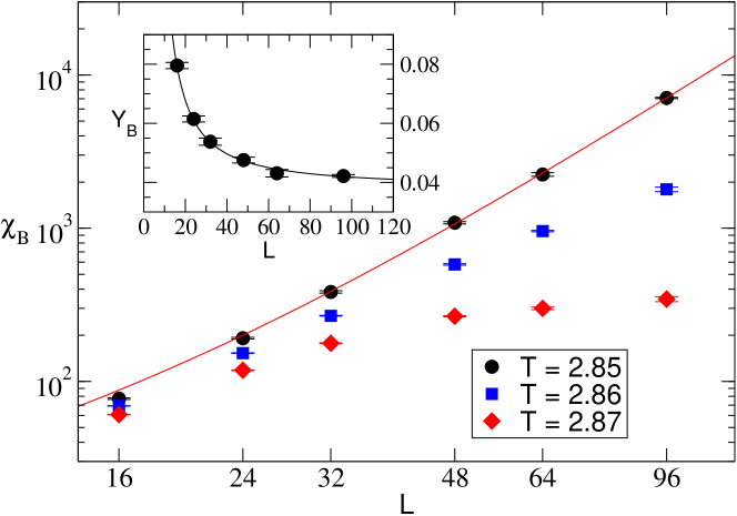
Figure 5: This figure shows $\chi_{B}$ as a function of $L$ at $\mu=0.3$ at three different temperatures close to the critical temperature. The inset shows that $Y_{B}$ goes to a constant as a function of $L$ at $T=2.85$. The solid line is a plot of eq. (33) with $\Delta=0.117$ and $a=2.4(3)$. Clearly, $\chi_{B}$ grows as $L^{3}$ at $T=2.85$ but begins to saturate at $T=2.87$ indicating that there is a transition between these two temperatures.

Figure 5 also shows $\chi_{B}$ at $T=2.86$ and $2.87$ as a function of $L$. Unlike the $\mu=0$ case, $\chi_{B}$ behaves monotonically suggesting that the transition could be second order. In order to check this we can verify if eq. (30b) is satisfied close to $T_{c}$. A fit of our data to this relation gives $T_{c}=2.85946(7)$, $\nu=0.60(2)$ $f_{0}=1.128(3)$ and $f_{1}=-0.161(3)$ with a $\chi^{2}/DOF=1$. In figure 6 (plot on the left), we show our data and the fit. In the inset of the figure we plot $\chi_{B}$ at $T=2.8594$. Since this value of $T$ is close to $T_{c}$ we expect $\chi_{B}=g_{0}L^{2-\eta}$ should describe the data reasonably well. Indeed a fit shows $g_{0}=0.306(8)$, $\eta=0.042(2)$ with a $\chi^{2}/DOF$ of $1.2$ and is shown as a solid line in the inset. The values of $F^{2}$, $\Delta^{2}$ and $M_{B}$ obtained from the infinite volume extrapolations must also satisfy

$$F^{2}=a_{0}(T_{c}-T)^{\nu},M_{B}=c_{0}(T-T_{c})\nu,\Delta^{2}=d_{0}(T_{c}-T)^{2\beta}.$$ (34)

Figure 6 (plot on the right) shows a combined fit of these three quantities as a function of $T$ using the value of $T_{c}$ obtained above. We find $\nu=0.610(6)$, $\beta=0.311(5)$, $a_{0}=0.70(1)$, $c_{0}=0.79(1)$ and $d_{0}=0.252(3)$ with a $\chi^{2}/DOF=1.3$. Note that these critical exponents do satisfy the hyper-scaling relation $\beta=(d-2+\eta)\nu/2$. Thus, our data strongly supports the existence of a second order transition.

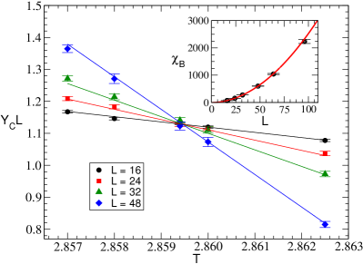
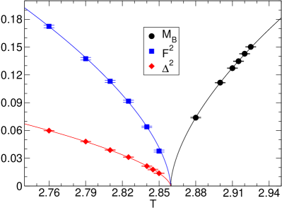
Figure 6: (Left) Plot of $Y_{C}L$ versus $T$ close to $T_{c}$ for various values of $L$. The solid lines are plots of $Y_{C}L=1.128-0.161(T-2.85946)L^{1/0.60}$. The inset shows $\chi_{B}$ as a function of $L$ at $T=2.8594$ and the solid line is a plot of $0.306L^{1.958}$. (Right) Plot of $M_{B}$, $F^{2}$,$\Delta^{2}$ versus $T$ close to $T_{c}$. The solid lines show the plots of eq. (34) with $a_{0}=0.70$, $c_{0}=0.79$,$d_{0}=0.252$, $\nu=0.610$, $\beta=0.311$ and $T_{c}=2.85946$.

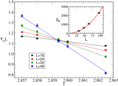
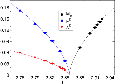
Figure 7: Same as figure 6 but now showing the solid lines show $O(2)$ scaling including corrections. (Left) The solid lines represent $Y_{C}L=2.321-1.26L^{-0.0218}-0.299(T-2.8590)L^{1/0.6715}$. The inset shows $\chi_{B}$ as a function of $L$ at $T=2.8590$ and the solid line is a plot of $0.302L^{1.962}$. (Right) The solid lines are plots to eqs.(35) with $a_{0}=4.8(5)$, $a^{\prime}_{0}=-0.8(1)$, $c_{0}=4.6(4)$, $c^{\prime}_{0}=-0.83(8)$, $d_{0}=2.1(1)$, $d^{\prime}_{0}=-0.89(5)$, $\nu=0.6715$, $\beta=0.3485$, $\omega=0.0218$.

Unfortunately, the above results are in contradiction with the expectation from section II.3, where it was argued that the critical behavior at $\mu\neq 0$ must be governed by three dimensional $XY$ universality class. This implies that we should have obtained $\nu=0.6715$, $\beta=0.3485$ and $\eta=0.0380$ Cam01 and not the exponents we found above. As discussed in section II.3, the problem is that in a model with $U(1)\times U(1)$ symmetry and collinear order, the corrections to the $XY$ scaling, due to the irrelevant direction in the $u,v$ plane (see section II.3), are rather large. Taking into account the leading corrections to scaling one expects $Y_{C}L=f_{0}+f^{\prime}_{0}L^{-\omega}+f_{1}(T-T_{c})L^{1/\nu}$ close to $T_{c}$ where $\omega=0.0218$ Vicari . The smallness of $\omega$ makes the corrections large for the lattice sizes we have explored. In fact we find that our data also fits well to this corrected form if we use the $XY$ critical exponents and the known value of $\omega$ in the fits. A combined four parameter fit of our data close to $T_{c}$ now yields $T_{c}=2.8590(3)$, $f_{0}=2.321(2)$, $f^{\prime}_{0}=-1.260(1)$, $f_{1}=-0.299(6)$ with a $\chi^{2}/DOF=1.6$. This fit is shown in figure 7 (the plot on the left). At $T=2.8590$, $\chi_{B}$ fits well to the form $g_{0}L^{2-\eta}$ when $\eta$ is fixed to $0.0380$. The fit gives $g_{0}=0.302(4)$ with a $\chi^{2}/DOF$ of $0.57$ (solid line in the inset of figure 7). When the scaling corrections are included in $F^{2}$, $\Delta^{2}$ and $M_{B}$ one gets

$$F = a_{0}(T_{c}-T)^{\nu}(1+a^{\prime}_{0}(T_{c}-T)^{\omega\nu}),\qquad$$ (35a)

$$M_{B} = c_{0}(T-T_{c})^{\nu}(1+c^{\prime}_{0}(T-T_{c})^{\omega\nu}),\qquad$$ (35b)

$$\Delta^{2} = d_{0}(T_{c}-T)^{2\beta}(1+d^{\prime}_{0}(T_{c}-T)^{\omega\nu}).$$ (35c)

Fixing $T_{c}=2.859$ and using the $XY$ critical exponents and $\omega$ as above, a combined fit again works very well and is shown in the plot on the right in figure 7. We get $a_{0}=4.8(5)$, $a^{\prime}_{0}=-0.8(1)$, $c_{0}=4.6(4)$, $c^{\prime}_{0}=-0.83(8)$, $d_{0}=2.1(1)$ and $d^{\prime}_{0}=-0.89(5)$ with a $\chi^{2}/DOF=1$.

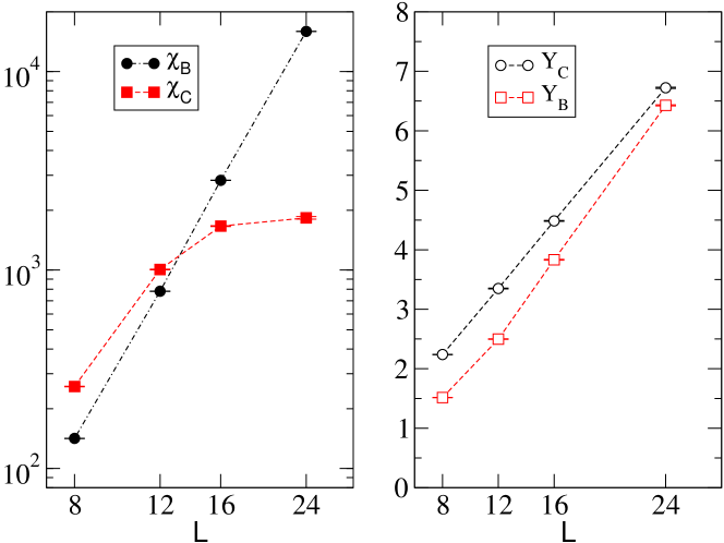
Figure 8: Results at $T=1.0$ and $\mu=0.01$. Note that $\chi_{B}$ grows with the volume while $\chi_{C}$ saturates. Both $Y_{C}$ and $Y_{B}$ grow linearly with $L$. The lines are drawn to guide the eye.

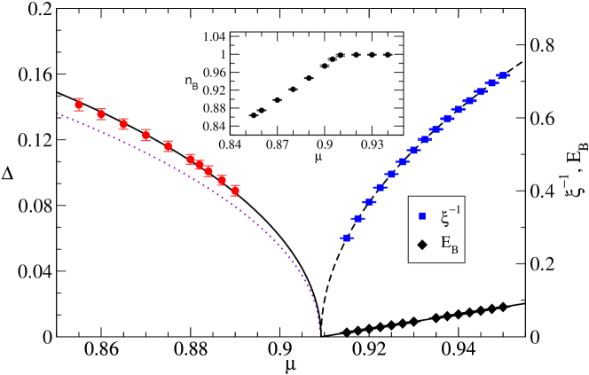
Figure 9: The figure shows our results for $\Delta$, $\xi^{-1}$ and $E_{B}$ as a function of $\mu$. For $\mu<\mu_{c}$ the dotted line is the mean field result for $\Delta$ given in eq. (37) and the solid line contains the one loop corrections. For $\mu>\mu_{c}$ the dashed line is the plot of $3.549\sqrt{\mu-\mu_{c}}$ and the solid line is the plot of $2(\mu-\mu_{c})$. We have used $\mu_{c}=0.90922$ here. The inset shows the baryon density $n_{B}$ as a function of $\mu$.

V.3 Zero Temperature

Next we turn to the physics at zero temperature. For this purpose we compute quantities with $L_{t}=L$ at $T=1.0$ for various values of $\mu$ and $L$. We now expect

$$\chi_{B}\sim\frac{\Delta^{2}}{2}L^{4}$$ (36)

where $\Delta=\langle\chi_{1}\chi_{2}\rangle=\langle\bar{\chi}_{2}\bar{\chi}_{1}\rangle\neq 0$. Note that since we use the same finite size scaling form in four and three dimensions, $\Delta$ is normalized differently here as compared to the finite temperature case. The chiral susceptibility $\chi_{C}$, must again saturate with $L$ at any non-zero value of $\mu$. Finally, due to our definitions (see eqs.(23), (25)) both the helicity modulus $Y_{C}$ and $Y_{B}$, grow linearly with $L$ for large $L$. These expectations emerge nicely in our calculations as can be seen in figure 8.

As the chemical potential increases the average number of baryons in the ground state increases. At some critical chemical potential $\mu_{c}$, the ground state has a baryon on every lattice site. Since the baryons behave as hard-core bosons, at $\mu_{c}$ there must be a phase transition to a phase where superfluidity is no longer present. We now focus on this phase transition. Renormalization group arguments show that this phase transition must be governed by mean field theory Fisher89 . A mean field analysis was performed recently in Nishida:2003uj and the critical chemical potential was found to be $\mu_{c}=0.5\cosh^{-1}(\sqrt{10})=0.909223..$. The diquark condensate was shown to be Comm1

$$\Delta=\sqrt{\frac{1}{18}\left(\sqrt{10}-\cosh(2\mu)\right)}$$ (37)

In order to check these results we have computed the diquark condensate $\Delta$ by fitting our $\chi_{B}$ data to the relation $\chi_{B}=\frac{\Delta^{2}}{2}[L^{4}+a^{\prime\prime}L^{2}+b^{\prime\prime}]$. Figure 9 shows our data along with the mean field result Nishida:2003uj and the result with one-loop corrections Jia06 . Clearly, the one-loop corrections are necessary before connection with mean field theory can be established.

The fact that this phase transition is driven due to the saturation of the lattice with baryons can be seen in the inset of figure 9, where the baryon density is plotted as a function of $\mu$. For $\mu>\mu_{c}$ it costs an energy $E_{B}$ to remove a baryon. This energy gap grows linearly as $(\mu-\mu_{c})$. Thus for $\mu>\mu_{c}$ one obtains a phase containing non-relativistic particles whose dispersion relation for small momenta looks like $E(p)=E_{B}+p^{2}/2M_{k}$ which leads to a spatial correlation length $\xi=1/\sqrt{2E_{B}M_{k}}$. Since we expect $\xi$ to scale as $1/\sqrt{(\mu-\mu_{c})}$ close to $\mu_{c}$ one expects the kinetic mass $M_{k}$ to be a constant. Figure 9 shows the plot of $E_{g}$ and $\xi^{-1}$ as a function of $\mu$. We find $\xi^{-1}=3.549(4)\sqrt{(\mu-0.90920(3))}$ with a $\chi^{2}/DOF=0.26$ and $E_{B}=2.000(2)(\mu-0.90922(1))$ with a $\chi^{2}/DOF=0.35$. Again $\mu_{c}$ is in excellent agreement with the mean field result which provides strong evidence that the phase transition is second order and belongs to the mean field universality class. From the behavior of $E_{B}$ and $\xi$ we find $M_{k}=3.12(5)$.

VI Discussion and Conclusions

In this work we constructed an efficient cluster algorithm and studied the phase structure of two color lattice QCD with massless staggered fermions in the strong coupling limit. We found that the finite temperature phase transition at zero chemical potential is weakly first order, while the same transition at an intermediate value of the chemical potential was second order. This second order transition was found to be in the universality class of the three dimensional $XY$ model as expected from theoretical arguments. However, in order to show this we needed to include the large corrections to scaling expected in the theory. The quantum phase transition at zero temperature between a baryon superfluid phase and a normal phase was also found to be second order in the mean field universality class. The physics in the normal phase was that of interacting non-relativistic particles. Based on these observations, we can attempt to draw the full diagram of two color QCD in the strong coupling limit. Our proposal is shown in figure 10.

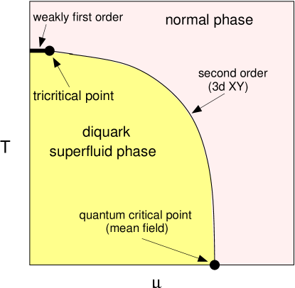
Figure 10: The phase diagram of two-color lattice QCD with staggered fermions at strong couplings.

It is important to understand how this phase diagram will change as we go to weaker couplings and towards the continuum limit. Clearly, when the four flavor nature of staggered fermions becomes important, it can begin to change significantly. However, for couplings that are currently explored, universality arguments suggest that the phase diagram will qualitatively remain the same although quantitatively the values of the critical points will mostlikely get affected. It is also interesting to ask why the transition at $\mu=0$ is so weak. As discussed in section II, renormalization group studies based on the $\epsilon$-expansion indicate that the transition will generically be a fluctuation driven first order transition Kawamura88 . Such a transition could be weak as we observe. On the other hand, recent work based on high order perturbation theory combined with resummation techniques do not rule out the possibility of a second order transition Prato . This means we are in the vicinity of a tricritical point and by changing some parameter in the theory we could change the transition to second order. When this occurs, it is likely that the weakly first order line in the above phase diagram will disappear. Such a scenario can in principle be investigated by introducing more tunable parameters within our model and by studying their effects on the order of the transition.

It is amusing to note that the above phase diagram is different from the standard phase diagram in QCD where the baryon chemical potential induces a first order transition instead of weakening it. This non-standard scenario was discussed in Philipsen:2005mj as a possibility in QCD and has also been seen in the potts model simulations Kim:2005ck . Finally, we note that the physics close to the quantum critical point is also interesting from the point of view of non-relativistic field theory. Since the model has a $U(1)\times U(1)$ symmetry, the low energy effective field theory here is richer than in a theory with a simple $U(1)$ particle number symmetry.

References

- (1) K. Rajagopal and F. Wilczek, arXiv:hep-ph/0011333.
- (2) T. Schafer, arXiv:hep-ph/0304281.
- (3) D. H. Rischke, Prog. Part. Nucl. Phys. 52, 197 (2004) [arXiv:nucl-th/0305030].
- (4) M. Alford, Prog. Theor. Phys. Suppl. 153, 1 (2004) [arXiv:nucl-th/0312007].
- (5) M. A. Stephanov, Prog. Theor. Phys. Suppl. 153, 139 (2004) [arXiv:hep-ph/0402115].
- (6) P. de Forcrand and O. Philipsen, Prog. Theor. Phys. Suppl. 153, 127 (2004).
- (7) M. P. Lombardo, Prog. Theor. Phys. Suppl. 153, 26 (2004) [arXiv:hep-lat/0401021].
- (8) C. R. Allton, S. Ejiri, S. J. Hands, O. Kaczmarek, F. Karsch, E. Laermann and C. Schmidt, Nucl. Phys. Proc. Suppl. 141, 186 (2005) [arXiv:hep-lat/0504011].
- (9) O. Philipsen, arXiv:hep-lat/0510077.
- (10) J. B. Kogut, M. A. Stephanov, D. Toublan, J. J. M. Verbaarschot and A. Zhitnitsky, Nucl. Phys. B 582, 477 (2000) [arXiv:hep-ph/0001171].
- (11) J. B. Kogut, M. A. Stephanov and D. Toublan, Phys. Lett. B 464, 183 (1999) [arXiv:hep-ph/9906346].
- (12) J. Wirstam, Phys. Rev. D 62, 045012 (2000) [arXiv:hep-ph/9912446].
- (13) C. Ratti and W. Weise, Phys. Rev. D 70, 054013 (2004) [arXiv:hep-ph/0406159].
- (14) J. T. Lenaghan, F. Sannino and K. Splittorff, Phys. Rev. D 65, 054002 (2002) [arXiv:hep-ph/0107099].
- (15) J. B. Kogut, J. Polonyi, H. W. Wyld and D. K. Sinclair, Nucl. Phys. B 265, 293 (1986).
- (16) J. B. Kogut, Nucl. Phys. B 290, 1 (1987).
- (17) O. Kaczmarek, F. Karsch and E. Laermann, Nucl. Phys. Proc. Suppl. 73, 441 (1999) [arXiv:hep-lat/9809059].
- (18) S. Hands, J. B. Kogut, M. P. Lombardo and S. E. Morrison, Nucl. Phys. B 558, 327 (1999) [arXiv:hep-lat/9902034].
- (19) S. Hands, I. Montvay, S. Morrison, M. Oevers, L. Scorzato and J. Skullerud, Eur. Phys. J. C 17, 285 (2000) [arXiv:hep-lat/0006018].
- (20) J. B. Kogut, D. K. Sinclair, S. J. Hands and S. E. Morrison, Phys. Rev. D 64, 094505 (2001) [arXiv:hep-lat/0105026].
- (21) J. B. Kogut, D. Toublan and D. K. Sinclair, Phys. Rev. D 68, 054507 (2003) [arXiv:hep-lat/0305003].
- (22) J. I. Skullerud, S. Ejiri, S. Hands and L. Scorzato, Prog. Theor. Phys. Suppl. 153, 60 (2004) [arXiv:hep-lat/0312002].
- (23) H. Kawamura, Phys. Rev. B38, 4916 (1988); erratum B42, 2610 (1990).
- (24) Y. Zhang, E. Demler and S. Sachdev, Phys. Rev. B66, 094501 (2002).
- (25) D.R.T. Jones, A. Love and M.A. Moore, J. Phys. C9, 743 (1976).
- (26) M. De Prato, A. Pelissetto, and E. Vicari, Phys. Rev. B 70, 214519 (2004).
- (27) D. H. Adams and S. Chandrasekharan, Nucl. Phys. B 662, 220 (2003) [arXiv:hep-lat/0303003].
- (28) J. M. Blairon, R. Brout, F. Englert and J. Greensite, Nucl. Phys. B 180, 439 (1981).
- (29) N. Kawamoto and J. Smit, Nucl. Phys. B 192, 100 (1981).
- (30) H. Kluberg-Stern, A. Morel and B. Petersson, Nucl. Phys. B 215, 527 (1983).
- (31) O. Martin and B. Siu, Phys. Lett. B 131, 419 (1983).
- (32) P. Rossi and U. Wolff, Nucl. Phys. B 248, 105 (1984).
- (33) U. Wolff, Phys. Lett. B 153, 92 (1985).
- (34) E. Dagotto, A. Moreo and U. Wolff, Phys. Rev. Lett. 57, 1292 (1986).
- (35) E. Dagotto, F. Karsch and A. Moreo, Phys. Lett. B 169, 421 (1986).
- (36) E. Dagotto, A. Moreo and U. Wolff, Phys. Lett. B 186, 395 (1987).
- (37) F. Karsch and K. H. Mutter, Nucl. Phys. B 313 (1989) 541.
- (38) J. U. Klatke and K. H. Mutter, Nucl. Phys. B 342, 764 (1990).
- (39) G. Boyd, J. Fingberg, F. Karsch, L. Karkkainen and B. Petersson, Nucl. Phys. B 376, 199 (1992).
- (40) B. Bringoltz and B. Svetitsky, Phys. Rev. D 68, 034501 (2003) [arXiv:hep-lat/0211018].
- (41) B. Bringoltz and B. Svetitsky, Phys. Rev. D 69, 014502 (2004) [arXiv:hep-lat/0310032].
- (42) B. Bringoltz, arXiv:hep-lat/0511058.
- (43) Y. Nishida, K. Fukushima and T. Hatsuda, Phys. Rept. 398, 281 (2004) [arXiv:hep-ph/0306066].
- (44) S. Chandrasekharan and F. J. Jiang, PoS LAT2005, 198 (2005) [arXiv:hep-lat/0509117].
- (45) M.P.A. Fisher, P.B. Weichman, G. Grinstein and D.S. Fisher, Phys. Rev. B40, 546 (1989).
- (46) P. Bak and D. Mukamel, Phys. Rev. B13, 5086 (1976).
- (47) A. Aharony, in: C. Domb, M.S. Green (Eds.), Phase Transitions and Critical Phenomena, Vol. 6, Academic Press, New York, p. 357 (1976).
- (48) A. Pelissetto and E. Vicari, Physics Reports 368 (2002) 549 727
- (49) E. Vicari, private communication.
- (50) O.F. Syljuasen and A.W. Sandvik, Phys. Rev. E 66 046701 (2002).
- (51) P. Hasenfratz and H. Leutwyler, Nucl. Phys. B 343, 241 (1990).
- (52) In the conference proceedings Chandrasekharan:2005dn , eq. (28) and eq. (29) were incorrect leading to the wrong normalization of . The correct normalization improves some of the fits.
- (53) S. Chandrasekharan and F. J. Jiang, Phys. Rev. D 68, 091501 (2003) [arXiv:hep-lat/0309025].
- (54) S. Chandrasekharan and C. G. Strouthos, Phys. Rev. D 68, 091502 (2003) [arXiv:hep-lat/0306034].
- (55) S. Chandrasekharan and C. G. Strouthos, Phys. Rev. Lett. 94, 061601 (2005) [arXiv:hep-lat/0410036].
- (56) M. Campostrini, M. Hasenbusch, A. Pelissetto, P. Rossi and E. Vicari, Phys. Rev. B63, 214503 (2001).
- (57) There is a factor of two mismatch in the formula quoted here and the one in Nishida:2003uj . The origin of this mismatch is the normalization of our kinetic term in eq. (1) as compared to the one in Nishida:2003uj .
- (58) F.-J. Jiang, under preparation for publication.
- (59) S. Kim, P. de Forcrand, S. Kratochvila and T. Takaishi, PoS LAT2005, 166 (2005) [arXiv:hep-lat/0510069].