Extracting $F_{\pi}$ from small lattices: unquenched results

Abstract

We calculate the response of the microscopic Dirac spectrum to an imaginary isospin chemical potential for QCD with two dynamical flavors in the chiral limit. This extends our previous calculation from the quenched to the unquenched theory. The resulting spectral correlation function in the $\epsilon$-regime provides here, too, a new and efficient way to measure $F_{\pi}$ on the lattice. We test the method in a hybrid Monte Carlo simulation of the theory with two staggered quarks.

I Introduction

A primary challenge for lattice gauge theory is the numerical determination of the low-energy constants of QCD with nearly massless $u$ and $d$ quarks. The chiral limit is a notoriously difficult problem on the lattice. Furthermore, one also has to face the issue of finite-volume effects, a problem that is compounded by the light quarks. A situation like this is best tackled head-on by means of finite-size scaling techniques, as is routinely done when the correlation length becomes comparable to the system size (such as near continuous phase transitions). Unfortunately, exact finite-size scaling functions for the chiral limit are not easy to come by. One notable exception is the so-called $\epsilon$-regime of QCD LS . It has been known for more than a decade Jac that this makes possible precise measurements of the infinite-volume chiral condensate $\Sigma=\langle\bar{\psi}\psi\rangle$ from simulations on small lattices. By definition, in the $\epsilon$-regime the linear extent $L$ of the box is smaller than the Compton wavelength $1/m_{\pi}$ of the pions, but much larger than $1/\Lambda_{\rm QCD}$. It is in this sense that the lattice required is small: Rather than demanding that the pion be contained by the lattice, one requires precisely that the lattice be too small for the pion.

In the $\epsilon$-regime the leading term of the effective partition function is a known function that is determined uniquely by the flavor symmetries and their spontaneous breaking. While this leads to an equally computable analytical expression for the condensate $\langle\bar{\psi}\psi\rangle$ that can be compared to lattice measurements Jac1 , a far more precise estimate comes from extracting $\Sigma$ from the analytical expressions for the distributions and correlations of the smallest eigenvalues of the Dirac operator. The universal predictions for different eigenvalue distributions according to the topological index $\nu$ and gauge group representation of the quarks DN have been checked in detail for both staggered and overlap fermions in a variety of studies with different color representations, mainly in quenched calculations (see, e. g., Refs. BB ; Jac for a partial list), but also with dynamical fermions BB1 ; DHNR .

Here we will consider the computation of the low-energy constant $F_{\pi}$, associated with the decay of pions. In the conventional approach $F_{\pi}$ is measured in a regime where the Compton wavelength of the pion is much smaller than the lattice size (see Fpi-quen for some recent quenched and Fpi-dyn for some recent dynamical calculations of $F_{\pi}$). We have recently presented a new method for extracting the pion decay constant $F_{\pi}$ from Dirac operator eigenvalues in the $\epsilon$-regime DHSS . In our first paper the focus was on quenched QCD. In this article, we extend this method to QCD with two dynamical light flavors, the physical $u$ and $d$ quarks.

In principle, all low-energy constants of QCD can be determined numerically from the spectrum of the Dirac operator. To leading order the spectrum depends only on the infinite-volume chiral condensate $\Sigma$, but higher order terms (in the counting of the $\epsilon$-expansion for the chiral Lagrangian LS ) give rise to measurable deviations. The idea of the improved method proposed in Ref. DHSS is to make use of an enlarged set of couplings provided by external fields. In particular we introduce a constant Abelian field that couples with opposite sign to the $u$ and $d$ quarks. This can be interpreted as an imaginary isospin chemical potential MT . Such a source turns out to have a dramatic effect on a certain spectral correlation function of the Dirac operator. It is this effect which allows for a very precise determination of $F_{\pi}$.

An alternative method is to use a real baryon chemical potential to extract the $F_{\pi}$-dependence of the microscopic spectral density. Recently quenched results based on this method have been reported OW . The analytical predictions for this method were derived in Ref. baryon ; SplitVerb2 . The advantage of our method is that the Dirac operator eigenvalues remain real, while a baryon chemical potential makes them (and the determinant) complex. The pion decay constant has also been measured from meson correlation functions in the $\epsilon$-regime (see $e.g.$ Fpi-ep ).

The outline of the paper is as follows. We first present the analytical result for the spectral correlation function whose dependence on $F_{\pi}$ is the backbone of our method. We then compare this prediction to the results of numerical simulations of QCD with two dynamical flavors, and use this to extract the value for $F_{\pi}$.

II Two Light Flavors: The Analytical Result

An imaginary isospin chemical potential leads us to consider two distinct Dirac operators and their eigenvalues for a given gauge potential $A$:

$$D_{+}\psi_{+}^{(n)} \equiv (\hbox to0.0pt{\raisebox{0.6458pt}{$\mskip 4.0mu/$}\hss}D(A)+i\mu_{\rm iso}\gamma_{0})\psi_{+}^{(n)}=i\lambda_{+}^{(n)}\psi_{+}^{(n)},$$ (1)

$$D_{-}\psi_{-}^{(n)} \equiv (\hbox to0.0pt{\raisebox{0.6458pt}{$\mskip 4.0mu/$}\hss}D(A)-i\mu_{\rm iso}\gamma_{0})\psi_{-}^{(n)}=i\lambda_{-}^{(n)}\psi_{-}^{(n)}.$$ (2)

Since the operators $D_{\pm}$ are anti-hermitian, the eigenvalues $\lambda_{+}^{(n)}$ and $\lambda_{-}^{(n)}$ lie on the real axis. This justifies the otherwise artificial use of an imaginary isospin chemical potential. Viewed in terms of external gauge potentials it is actually the natural choice, corresponding to a constant real Abelian gauge potential $A_{0}=\mu_{\rm iso}$.

We consider the mixed two-point spectral correlation function of the Dirac operators $D_{\pm}$. The formulae for the quenched theory were given in Ref. DHSS ; here we briefly present the corresponding expressions for two dynamical flavors. The mixed two-point function, which depends on the two light masses $m_{u}$ and $m_{d}$ and on $\mu_{\rm iso}$, is defined as

$$\rho^{(2)}(\lambda_{+},\lambda_{-},m_{u},m_{d};i\mu_{\rm iso})\equiv\Bigl{\langle}\sum_{n}\delta(\lambda_{+}-\lambda_{+}^{(n)})\sum_{l}\delta(\lambda_{-}-\lambda_{-}^{(l)})\Bigr{\rangle}-\Bigl{\langle}\sum_{n}\delta(\lambda_{+}-\lambda_{+}^{(n)})\Bigr{\rangle}\Bigl{\langle}\sum_{l}\delta(\lambda_{-}-\lambda_{-}^{(l)})\Bigr{\rangle},$$ (3)

where the brackets denote the average over the QCD partition function with two flavors and $\mu_{\rm iso}\neq 0$,

$${Z}_{2}(m_{u},m_{d};i\mu_{\rm iso}) = \int[{\rm d}A]_{\nu}\det(D_{+}+m_{u})\det(D_{-}+m_{d})\,e^{-S_{\rm YM}(A)}.$$ (4)

The index $\nu$ on the measure indicates that this is the partition function in a sector where the gauge fields have topological charge $\nu$. Keeping fixed the scaling variables

$$\xi_{\pm}=\lambda_{\pm}\Sigma V,\quad\hat{m}_{u,d}=m_{u,d}\Sigma V,\quad\hat{\mu}_{\rm iso}=\mu_{\rm iso}F_{\pi}\sqrt{V},$$ (5)

as $V\rightarrow\infty$, we define the microscopic two point correlation function

$$\rho^{(2)}_{s}(\xi_{+},\xi_{-},\hat{m}_{u},\hat{m}_{d};i\hat{\mu}_{\rm iso})\equiv\lim\frac{1}{\Sigma^{2}V^{2}}\,\rho^{(2)}\Big{(}\frac{\xi_{+}}{\Sigma V},\frac{\xi_{-}}{\Sigma V},\frac{\hat{m}_{u}}{\Sigma V},\frac{\hat{m}_{d}}{\Sigma V};i\frac{\hat{\mu}_{\rm iso}}{F_{\pi}\sqrt{V}}\Big{)}.$$ (6)

This spectral correlation function $\rho^{(2)}$ can be obtained from the mixed “partially quenched” scalar susceptibility,

$$\chi(m_{+},m_{-},m_{u},m_{d};i\mu_{\rm iso})\equiv\left\langle\,{\rm tr}\,\frac{1}{D_{+}+m_{+}}\,{\rm tr}\,\frac{1}{D_{-}+m_{-}}\right\rangle-\left\langle\,{\rm tr}\,\frac{1}{D_{+}+m_{+}}\right\rangle\left\langle\,{\rm tr}\,\frac{1}{D_{-}+m_{-}}\right\rangle,$$ (7)

which possesses the spectral representation

$$\chi(m_{+},m_{-},m_{u},m_{d};i\mu_{\rm iso})=\left\langle\sum_{n}\frac{1}{i\lambda_{+}^{(n)}+m_{+}}\sum_{l}\frac{1}{i\lambda_{-}^{(l)}+m_{-}}\right\rangle-\left\langle\sum_{n}\frac{1}{i\lambda_{+}^{(n)}+m_{+}}\right\rangle\left\langle\sum_{l}\frac{1}{i\lambda_{-}^{(l)}+m_{-}}\right\rangle.$$ (8)

The desired correlation function follows from the double discontinuity across the imaginary axis DOTV ,

$$\rho^{(2)}(\lambda_{+},\lambda_{-},m_{u},m_{d};i\mu_{\rm iso}) = \frac{1}{4\pi^{2}}{\rm Disc}\,\chi(m_{+},m_{-},m_{u},m_{d};i\mu_{\rm iso})|_{m_{+}=i\lambda_{+}\atop m_{-}=i\lambda_{-}}$$ (10)

$$= \frac{1}{4\pi^{2}}\lim_{\epsilon\rightarrow 0^{+}}[\chi(i\lambda_{+}+\epsilon,i\lambda_{-}+\epsilon,m_{u},m_{d};i\mu_{\rm iso})-\chi(i\lambda_{+}-\epsilon,i\lambda_{-}+\epsilon,m_{u},m_{d};i\mu_{\rm iso})$$

$$\qquad-\chi(i\lambda_{+}+\epsilon,i\lambda_{-}-\epsilon,m_{u},m_{d};i\mu_{\rm iso})+\chi(i\lambda_{+}-\epsilon,i\lambda_{-}-\epsilon,m_{u},m_{d};i\mu_{\rm iso})].$$

The power of the $\epsilon$-regime is that this function, $\rho^{(2)}$, can be expressed in closed analytical form.

The mixed scalar susceptibility (7) involves two additional fermion species, with mass $m_{+}$ and $m_{-}$, coupled as well to the external field $\mu_{\rm iso}$. This quantity thus has to be evaluated in a theory with four fermion species, of which only two become physical (the $u$ and $d$ quarks), while the remaining two are quenched away and serve as sources for the two eigenvalues involved in the two-point correlation function. In order to do this we will use the replica method (see, e.g., DS ). We have

$$\chi(m_{+},m_{-},m_{u},m_{d};i\mu_{\rm iso}) = \lim_{n\rightarrow 0}\frac{1}{n^{2}}\partial_{m_{+}}\partial_{m_{-}}\log Z_{2n,2}(m_{+},m_{-},m_{u},m_{d};i\mu_{\rm iso}),$$ (11)

where the generating functionals $Z_{2n,2}$ have $2n$ replica flavors besides the two flavors of mass $m_{u}$ and $m_{d}$,

$${Z}_{2n,2}(m_{+},m_{-},m_{u},m_{d};i\mu_{\rm iso}) = \int[{\rm d}A]_{\nu}\left[\det(D_{+}+m_{+})\det(D_{-}+m_{-})\right]^{n}$$ (12)

$$\quad\times\det(D_{+}+m_{u})\det(D_{-}+m_{d})\,e^{-S_{\rm YM}(A)}.$$

Half of the replica flavors have mass $m_{+}$ and chemical potential $+i\mu_{\rm iso}$ while the other half have mass $m_{-}$ and chemical potential $-i\mu_{\rm iso}$.

In the $\epsilon$-regime the leading terms of the effective partition functions satisfy a string of Toda lattice equations which can be used to extract the replica limit K ; SplitVerb1 . Specifically SplitVerb2 ,

$$\hat{m}_{+}\partial_{\hat{m}_{+}}\hat{m}_{-}\partial_{\hat{m}_{-}}\log Z_{2n,2}(\hat{m}_{+},\hat{m}_{-},\hat{m}_{u},\hat{m}_{d};i\hat{\mu}_{\rm iso})$$ (13)

$$=4n^{2}(\hat{m}_{+}\hat{m}_{-})^{2}\frac{Z_{2n+2,2}(\hat{m}_{+},\hat{m}_{-},\hat{m}_{u},\hat{m}_{d};i\hat{\mu}_{\rm iso})Z_{2n-2,2}(\hat{m}_{+},\hat{m}_{-},\hat{m}_{u},\hat{m}_{d};i\hat{\mu}_{\rm iso})}{[Z_{2n,2}(\hat{m}_{+},\hat{m}_{-},\hat{m}_{u},\hat{m}_{d};i\hat{\mu}_{\rm iso})]^{2}}.$$

Taking the replica limit (11) of this Toda lattice equation we get

$$\chi(\hat{m}_{+},\hat{m}_{-},\hat{m}_{u},\hat{m}_{d};i\hat{\mu}_{\rm iso})=4\hat{m}_{+}\hat{m}_{-}\frac{Z_{2,2}(\hat{m}_{+},\hat{m}_{-},\hat{m}_{u},\hat{m}_{d};i\hat{\mu}_{\rm iso})Z_{2,-2}(\hat{m}_{u},\hat{m}_{d}|\hat{m}_{+},\hat{m}_{-};i\hat{\mu}_{\rm iso})}{[Z_{2}(\hat{m}_{u},\hat{m}_{d};i\hat{\mu}_{\rm iso})]^{2}}.$$ (14)

We need three different effective partition functions to evaluate the right hand side of this equation. Of these, the two that involve only positive numbers of flavors are of the form

$$Z_{2n,2}(\hat{m}_{+},\hat{m}_{-},\hat{m}_{u},\hat{m}_{d};i\hat{\mu}_{\rm iso})=\int_{U\in U(2n+2)}dU\det(U)^{\nu}e^{\frac{1}{4}VF_{\pi}^{2}\mu_{\rm iso}^{2}{\rm Tr}[U,B][U^{\dagger},B]+\frac{1}{2}\Sigma V{\rm Tr}(M^{\dagger}U+MU^{\dagger})}\,,$$ (15)

where $B={\rm diag}(1_{n+1},-1_{n+1})$ and $M={\rm diag}(m_{+},\ldots,m_{+},m_{u},m_{-},\ldots,m_{-},m_{d})$. In particular,

$$Z_{2}(\hat{m}_{+},\hat{m}_{-};i\hat{\mu}_{\rm iso}) = e^{-2\hat{\mu}_{\rm iso}^{2}}\int_{0}^{1}dt\,te^{2\hat{\mu}_{\rm iso}^{2}t^{2}}I_{\nu}(t\hat{m}_{+})I_{\nu}(t\hat{m}_{-}),$$ (16)

where we have defined $\hat{m}_{\pm}=m_{\pm}\Sigma V$, while an explicit analytical expression for $Z_{2,2}$ can be obtained from Ref. AFV ,

$$Z_{2,2}(\hat{m}_{+},\hat{m}_{-},\hat{m}_{u},\hat{m}_{d};i\hat{\mu}_{\rm iso})=\frac{1}{(\hat{m}_{+}^{2}-\hat{m}_{u}^{2})(\hat{m}_{-}^{2}-\hat{m}_{d}^{2})}\,\left|\begin{array}[]{cc}Z_{2}(\hat{m}_{+},\hat{m}_{-};i\hat{\mu}_{\rm iso})&Z_{2}(\hat{m}_{+},\hat{m}_{d};i\hat{\mu}_{\rm iso})\\[2.0pt] Z_{2}(\hat{m}_{u},\hat{m}_{-};i\hat{\mu}_{\rm iso})&Z_{2}(\hat{m}_{u},\hat{m}_{d};i\hat{\mu}_{\rm iso})\end{array}\right|.$$ (19)

The remaining partition function $Z_{2,-2}$ on the right hand side of Eq. (14) is the most difficult part. It involves two fermion species (the two physical $u$ and $d$ quarks) and in addition $-2$ flavors, i.e., two bosons. The resulting effective partition function is an integral over a graded group. Deferring the technical discussion of this to a forthcoming paper nextpaper , we quote the final result,

$$Z_{2,-2}(\hat{m}_{u},\hat{m}_{d}|\hat{m}_{+},\hat{m}_{-};i\hat{\mu}_{\rm iso})=\left|\begin{array}[]{cc}(\hat{m}_{u}^{2}-\hat{m}_{+}^{2})Z_{2}(\hat{m}_{u},\hat{m}_{d};i\hat{\mu}_{\rm iso})&Z_{1,-1}(\hat{m}_{d}|\hat{m}_{-})\\[2.0pt] -Z_{1,-1}(\hat{m}_{u}|\hat{m}_{+})&(\hat{m}_{d}^{2}-\hat{m}_{-}^{2})Z_{-2}(\hat{m}_{+},\hat{m}_{-};i\hat{\mu}_{\rm iso})\end{array}\right|.$$ (22)

In Eq. (22) the ($\mu$-independent) partition function with one fermion and one boson is given by

$$Z_{1,-1}(\hat{x}|\hat{y})=\hat{x}I_{1}(\hat{x})K_{0}(\hat{y})+\hat{y}K_{1}(\hat{y})I_{0}(\hat{x}),$$ (23)

and the partition function with two bosons is

$$Z_{-2}(\hat{x},\hat{y};i\hat{\mu}_{\rm iso})=e^{2\hat{\mu_{\rm iso}}^{2}}\int_{1}^{\infty}dt\,te^{-2\hat{\mu}_{\rm iso}^{2}t^{2}}K_{\nu}(t\hat{x})K_{\nu}(t\hat{y}).$$ (24)

where $\hat{x}=x\Sigma V$ and $\hat{y}=y\Sigma V$.

We can finally compute the required two-point correlation function (6) by means of the discontinuity (10). The result is

$$\rho^{(2)}_{s}(\xi_{+},\xi_{-},\hat{m}_{u},\hat{m}_{d};i\hat{\mu}_{\rm iso}) = \xi_{+}\xi_{-}\left[\int_{0}^{1}dt\,te^{2\hat{\mu}_{\rm iso}^{2}t^{2}}I_{\nu}(t\hat{m}_{u})I_{\nu}(t\hat{m}_{d})\right]^{-2}$$

$$\times\left[\int_{0}^{1}dt\,te^{2\hat{\mu}_{\rm iso}^{2}t^{2}}J_{\nu}(t\xi_{+})J_{\nu}(t\xi_{-})\int_{0}^{1}dt\,te^{2\hat{\mu}_{\rm iso}^{2}t^{2}}I_{\nu}(t\hat{m}_{u})I_{\nu}(t\hat{m}_{d})\right.$$

$$\qquad-\left.\int_{0}^{1}dt\,te^{2\hat{\mu}_{\rm iso}^{2}t^{2}}I_{\nu}(t\hat{m}_{u})J_{\nu}(t\xi_{-})\int_{0}^{1}dt\,te^{2\hat{\mu}_{\rm iso}^{2}t^{2}}J_{\nu}(t\xi_{+})I_{\nu}(t\hat{m}_{d})\right]$$

$$\times\left[\int_{0}^{1}dt\,te^{2\hat{\mu}_{\rm iso}^{2}t^{2}}I_{\nu}(t\hat{m}_{u})I_{\nu}(t\hat{m}_{d})\int_{1}^{\infty}dt\,te^{-2\hat{\mu}_{\rm iso}^{2}t^{2}}J_{\nu}(t\xi_{+})J_{\nu}(t\xi_{-})\right.$$

$$\left.+\frac{[\hat{m}_{u}I_{\nu+1}(\hat{m}_{u})J_{\nu}(\xi_{+})+\xi_{+}J_{\nu+1}(\xi_{+})I_{\nu}(\hat{m}_{u})]\,[\hat{m}_{d}I_{\nu+1}(\hat{m}_{d})J_{\nu}(\xi_{-})+\xi_{-}J_{\nu+1}(\xi_{-})I_{\nu}(\hat{m}_{d})]}{(\xi_{+}^{2}+\hat{m}_{u}^{2})(\xi_{-}^{2}+\hat{m}_{d}^{2})}\right].$$

For a numerical evaluation it is advantageous to rewrite the improper integral appearing in the fourth line as

$$\int_{1}^{\infty}dt\,te^{-2\hat{\mu}_{\rm iso}^{2}t^{2}}J_{\nu}(t\xi_{+})J_{\nu}(t\xi_{-})=\frac{1}{4\hat{\mu}_{\rm iso}^{2}}\exp\left(-\frac{\xi_{+}^{2}+\xi_{-}^{2}}{8\hat{\mu}_{\rm iso}^{2}}\right)I_{\nu}\left(\frac{\xi_{+}\xi_{-}}{4\hat{\mu}_{\rm iso}^{2}}\right)-\int_{0}^{1}dt\,te^{-2\hat{\mu}_{\rm iso}^{2}t^{2}}J_{\nu}(t\xi_{+})J_{\nu}(t\xi_{-}).$$ (26)

In exact analogy to the quenched case DHSS , the correlation function (II) changes dramatically when $\mu_{\rm iso}$ is made non-zero. A fit to Monte Carlo data with $\mu_{\rm iso}\not=0$ using Eq. (II) will then readily produce a measurement of $F_{\pi}$.

III Numerical Results

We demonstrate our method by applying it to the eigenvalue correlation function calculated for SU(3) lattice gauge theory with two staggered fermions of equal mass $m_{u}=m_{d}\equiv m$. The gauge action is the standard plaquette action and unimproved staggered operators are used throughout. This theory has an exact U(2)$\times$U(2) symmetry; while it represents eight tastes in the continuum limit, we work far from the continuum limit, at a strong coupling $\beta=4.2$, in order to stay on the confining side of bulk and finite-temperature phase transitions 8flavors . In addition, and since we only aim at illustrating the method here, this rather strong coupling provides us with an unambiguous number of pseudo-Goldstone modes. At the coupling considered, two staggered fermions give rise to spontaneous chiral symmetry breaking of the form U(2)$\times$U(2)$\rightarrow$U(2). The staggered theory at this coupling thus appears to be “insensitive” to gauge field topology (see for instance DHNR_topo ): The additional U(1) factor in the coset dictates that we must compare our numerical results with $\nu=0$ in Eq. (II).

We ran the exact Hybrid Monte Carlo algorithm HMC on lattices with volume $V=4^{4}$ and $6^{4}$, setting $\mu_{\rm iso}=0.0125$ and 0.0055, respectively, in order to keep constant the scaling variable $\hat{\mu}_{\rm iso}$. We studied the cases $m=0.01$ and 0.025 for the smaller volume, and correspondingly $m=0.002$ and 0.005 in the larger volume. Note that the scaling variable $\hat{m}=m\Sigma V$ is fixed and $m_{\pi}L\lesssim 1$ (cf. table 2). An idea of the size of the simulation can be gotten from the run parameters listed in Table 1. We note that our method requires very small quark masses and hence many CG iterations (typically $10^{4}$ for the smaller mass in $V=6^{4}$, restarting every 500) for inverting the fermion matrix; the restriction to small volume, while allowing easy replication of the simulation for many processors, precludes gaining any advantage from true parallel computation.

$V$	${\it m}$	trajectories	$dt$	steps/trajectory	trajectories/measurement
$4^{4}$	$0.01$	$4000$	$0.0067$	150	1
$4^{4}$	$0.025$	$4000$	$0.0125$	80	1
$6^{4}$	$0.002$	$27960$	$0.001$	100	5
$6^{4}$	$0.005$	$5135$	$0.001$	200	5

Table 1: Run parameters for the Hybrid Monte Carlo simulations.

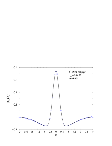
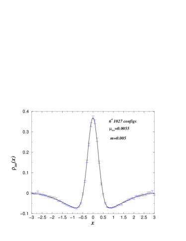
Figure 1: The integrated correlation function (27) with $\tilde{\xi}_{\rm min}=5$ and $\tilde{\xi}_{\rm max}=55$ for the ensembles with $V=6^{4}$ and $\mu_{\rm iso}=0.0055$. Left: $m=0.002$. The curve is the result of a fit with $\Sigma=0.3200\pm 0.0005$ and $F_{\pi}=0.3379\pm 0.0018$, with $\chi^{2}/\textit{dof}=1.33$. Right: $m=0.005$. The fit parameters are $\Sigma=0.3212\pm 0.0012$ and $F_{\pi}=0.3384\pm 0.0025$, with $\chi^{2}/\textit{dof}=1.13$.

As discussed in DHSS , when extracting physical observables we must keep in mind that the continuum theory describes 4 tastes of quark. Therefore, to determine the values of $F_{\pi}$ and $\Sigma$ from the staggered eigenvalue spectrum we must replace $V$ in the analytical predictions by 4$V$.

We begin with our main numerical result, the pion decay constant $F_{\pi}$. In order to improve the statistics we consider the integrated correlation function

$$\rho^{(2)}_{\rm int}(x)\equiv\int_{\xi_{\rm min}}^{\xi_{\rm max}}{\rm d}\xi\,\rho^{(2)}_{s}(\xi+x,\xi,\hat{m}_{u},\hat{m}_{d};i\hat{\mu}_{\rm iso}).$$ (27)

In Fig. 1 we show this integrated correlation function as measured on our $6^{4}$ ensemble, for both masses. The curves are fits to Eq. (27) via Eq. (II), see Table 2. The weighted averages of the fit parameters for the two data sets are $\Sigma=0.3204\pm 0.0004$ and $F_{\pi}=0.3381\pm 0.0010$, in lattice units. There are a number of other ways to determine $\Sigma$ from the eigenvalue densities and correlations; we will see that the value just obtained is consistent with other features of the spectra.

We now proceed to study the sensitivity of the correlation function to the mass. Since the mass affects mainly low-lying eigenvalues, this sensitivity is greatest when the correlation function is not integrated. We show in Fig. 2 the measured correlation function with one eigenvalue fixed at $\xi_{-}=4$. For each data set we compare to theoretical curves [Eq. (II)] with masses corresponding to the two chosen values of $m$ in the simulation, as well as to infinitely high mass (the quenched theory). We set $\Sigma$ and $F_{\pi}$ to the values obtained in the fits shown in Fig. 1, for each mass separately. It is clear that the effect of the mass in the analytical prediction is consistent with the data and inconsistent with the quenched result. It would take, however, a somewhat greater number of configurations to get a precise test of the mass dependence.

$V$	$m$	$F_{\pi}$	$\Sigma$	$m_{\pi}/F_{\pi}$	$m_{\pi}L$
$6^{4}$	0.002	$0.3379\pm 0.0018$	$0.3200\pm 0.0005$	$0.3133$	0.6354
$6^{4}$	0.005	$0.3384\pm 0.0025$	$0.3212\pm 0.0012$	$0.4949$	1.005

Table 2: Results of the data analysis. To extract the ratio $m_{\pi}/F_{\pi}$ we used the GOR-relation $m_{\pi}^{2}F_{\pi}^{2}=2m\Sigma$.

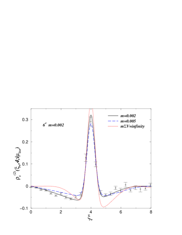
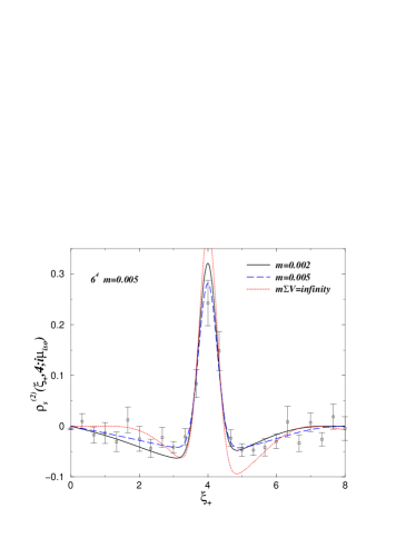
Figure 2: The correlation function (6), with $\xi_{-}$ fixed at 4, measured in the ensembles with $V=6^{4}$. Left: $m=0.002$. Right: $m=0.005$. The curves are Eq. (II) with $m=0.002$ (solid), 0.005 (dashed), and $\infty$ (dotted).

The scaling properties of the $\epsilon$ regime can be studied by comparing distributions for the two volumes. We begin with the eigenvalue density shown in Fig. 3. For the larger volume (right hand figure) the density as expected rises to a constant level (by convention the value reached should be $1/\pi$ as indicated by the horizontal line). The fall-off around the value $\xi=80$ occurs since only the lowest 24 eigenvalues have been computed. On the other hand the eigenvalue density in the smaller volume (left hand figure) only briefly remains at the plateau of height $1/\pi$. Thus it is not advisable to consider the integrated correlation function over the entire range of the 24 eigenvalues computed. In Fig. 4 we consider rather the correlation function with $\xi_{-}$ fixed at the value 4. Since we have chosen the quark masses such that $mV$ is fixed, the analytical curves shown are identical to those in Fig. 2. The general agreement confirms the expected scaling behavior.

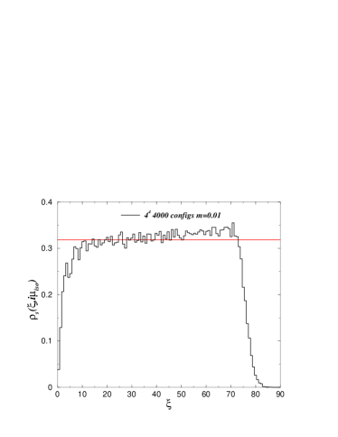
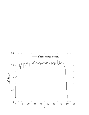
Figure 3: The eigenvalue density of the 24 lowest eigenvalues measured for the smaller scaled mass: $V=4^{4}$, $m=0.01$ (left) and $V=6^{4}$, $m=0.002$ (right). The horizontal line in each case is at $\rho_{s}=1/\pi$. For $V=4^{4}$ the eigenvalue density only remains briefly at the height $1/\pi$ whereas for $V=6^{4}$ all of the first 24 eigenvalues are within this plateau.

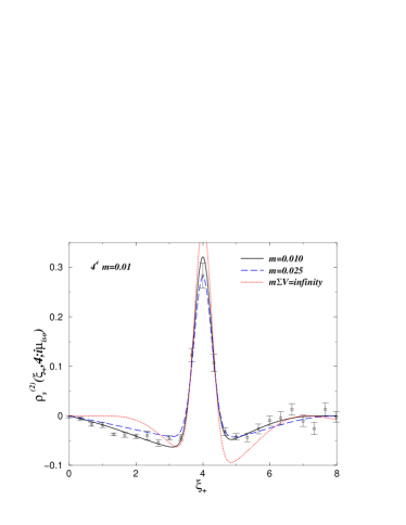
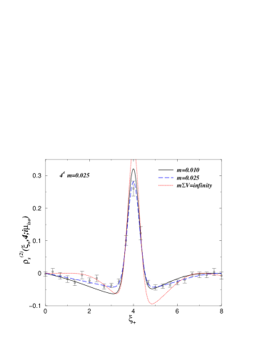
Figure 4: The correlation function (3), with $\xi_{-}$ fixed at 4, for $V=4^{4}$; $m=0.01$ (left) to be compared with the full curve and $m=0.025$ (right) to be compared with the dashed curve. The curves are obtained from (II) with $\Sigma$ and $F_{\pi}$ as determined in Fig. 1. The dotted curve indicates the quenched result.

Finally we take a brief look at the case where $\mu=0$. In this case the operators $D_{+}$ and $D_{-}$ are identical and the correlation function consequently has a delta-function peak at equal arguments. In Fig. 5 we show the integrated correlation function at $\mu_{\rm iso}=0$ as obtained on the $6^{4}$ lattice at mass $m=0.002$ along with the analytical prediction, using the value of $\Sigma$ determined in Fig. 1. The consistency with the data is a non-trivial cross check of the value of $\Sigma$ obtained in Fig. 1. The delta-function at $\xi_{+}=\xi_{-}$ is not shown. As $\mu_{\rm iso}$ is turned to a non-zero value the delta function peak gets smeared into a broader peak around zero as in Fig. 1. It is the fit to the shape of this broader peak that allows us to determine $F_{\pi}$.

Figure 5: The integrated correlation function at $\mu_{\rm iso}=0$, for $V=6^{4}$; $m=0.002$. The delta function at $x=0$ is not shown. The comparison with the analytic curve uses the value of $\Sigma$ determined in Fig. 1.

IV Summary

We have demonstrated that $F_{\pi}$ can be extracted with high precision from small lattices in unquenched lattice QCD. The approach exploits the dramatic dependence of the universal microscopic correlation functions on $F_{\pi}$. This dependence enters through the coupling to an external vector field in form of an imaginary isospin chemical potential. The derivation of the analytical results used here is quite involved and will be presented in nextpaper . We have performed appropriate two flavor lattice simulations, and the numerical results have been shown to agree with our analytical predictions. This agreement has allowed us to extract $F_{\pi}$ in lattice units. See Table 2 for a summary.

In this first study of the method with dynamical fermions we have worked with an unimproved staggered action. It would be of great interest to perform a simulation with actions suffering less severely from scaling violations, thus allowing to quote a result for $F_{\pi}$ in physical units.