DFUP-TH/2006-3, GEF-TH-2006-03

TOPOLOGY ON THE LATTICE

We review the method developed in Pisa to determine the topological susceptibility in lattice QCD and present a collection of new and old results obtained by the method.

1 Introduction

This article is dedicated to the study of topological properties of QCD on the lattice. We will describe the method developed in Pisa to measure the topological susceptibility on the lattice which is usually known as field–theoretical method and we will review results obtained by the method together with some recent applications.

Topology is a difficult subject to be studied on the lattice because from a strictly mathematical point of view it cannot be defined on a discrete space. Its meaning is recovered in the continuum limit, where the physical scale gets well separated from the ultraviolet (UV) one. The topological susceptibility enters in many contexts of QCD phenomenology $\!{}^{{\bf?},{\bf?},{\bf?},{\bf?},{\bf?}}$. It can be treated as usual expectation values of field operators in Quantum Field Theory. In this approach one does not try to assign a definite topological sector to each gauge field configuration. Instead appropriate renormalization constants are used to relate the lattice averages to the corresponding continuum ones. The method developed in Pisa consists in defining the renormalizations and in giving a prescription to compute them on the lattice, as one would do for any other field–theoretical expectation value. We will review this method in Section 2.

In Section 3 we collect some results obtained in the past by using the field–theoretical method in QCD at zero and finite temperature, with and without dynamical quarks. In Section 4 we present new results concerning the application of the method at finite temperature on anisotropic lattices and at finite density. A feature of these last results is that several determinations of the topological susceptibility are obtained with a fixed UV cutoff and this fact greatly reduces the number of renormalization constants required in the computation and makes the method even more practical and beautiful.

We have written this article to celebrate the 70th birthday of Adriano Di Giacomo: the study of topology on the lattice is surely one of the leading interests in his research activity, an interest which both of the authors have been lucky enough to share with him.

2 The topological susceptibility

The topological susceptibility $\chi$ is defined as the zero momentum two–point function of the topological charge density operator $q(x)$

$$\chi \equiv \frac{\langle Q^{2}\rangle}{V}=\int\hbox{d}^{4}x\;\langle q(x)q(0)\rangle\;,\;\;\;\;\;Q=\int\hbox{d}^{4}x\;q(x)\;,$$ (1)

$$q(x) = {g^{2}\over 64\pi^{2}}\epsilon_{\mu\nu\rho\sigma}F_{\mu\nu}^{a}(x)F_{\rho\sigma}^{a}(x)\;\;.$$ (2)

It contains information about the dependence of the QCD free energy on the topological $\theta$ parameter around $\theta=0$,

$$\chi=-\frac{1}{V}\frac{d^{2}}{d\theta^{2}}\ln Z(\theta)|_{\theta=0}\;,\;\;\;\;\;Z(\theta)=\int[dA]\;e^{-\int d^{4}x{\cal L_{QCD}}(x)}\;e^{i\theta\,Q}$$ (3)

and it enters in various aspects of QCD phenomenology by regulating the realization of the $U(1)_{A}$ axial symmetry. For instance, its value in the pure gauge theory is directly related, at the leading order in $1/N_{c}$ ($N_{c}$ is the number of colours), to the mass of the $\eta^{\prime}$ meson by the Witten–Veneziano mechanism $\!{}^{{\bf?},{\bf?}}$, which predicts $\chi\approx(180\,{\rm MeV})^{4}$.

Topological properties of QCD are of non–perturbative nature: lattice simulations are therefore the natural tool to investigate them. On the lattice a discretized gauge invariant topological charge density operator $q_{L}(x)$ can be defined, and a related topological charge $Q_{L}=\sum_{x}q_{L}(x)$, with the only requirement about the formal continuum limit $\lim_{a\to 0}q_{L}(x)=a^{4}q(x)$ where $a$ is the lattice spacing. A commonly used definition is $\!{}^{{\bf?}}$

$$q_{L}(x)={{-1}\over{2^{9}\pi^{2}}}\sum_{\mu\nu\rho\sigma=\pm 1}^{\pm 4}{\widetilde{\epsilon}}_{\mu\nu\rho\sigma}\hbox{Tr}\left(\Pi_{\mu\nu}(x)\Pi_{\rho\sigma}(x)\right)\;,$$ (4)

where $\Pi_{\mu\nu}(x)$ is the plaquette operator in the $\mu\nu$ plane, ${\widetilde{\epsilon}}_{\mu\nu\rho\sigma}$ is the Levi–Civita tensor for positive directions and is otherwise defined by the rule ${\widetilde{\epsilon}}_{\mu\nu\rho\sigma}=-{\widetilde{\epsilon}}_{(-\mu)\nu\rho\sigma}$.

A proper renormalization must be performed when going towards the continuum limit. In spite of the formal limit, the discretized topological charge density renormalizes multiplicatively $\!{}^{{\bf?},{\bf?}}$ (in presence of dynamical fermions also additive renormalizations can be present, see next Section)

$$q_{L}(x)=Z(\beta)a^{4}(\beta)q(x)+O(a^{6})\;,$$ (5)

with a renormalization constant $Z(\beta)$ which is a finite function of the lattice bare coupling $\beta=2N_{c}/g_{0}^{2}$, approaching 1 as $\beta\to\infty$.

When defining the topological susceptibility, further renormalizations can appear. Indeed, already the continuum definition of Eq. (2) involves the product of two operators $q(x)$ at the same point. Part of this contact term is necessary to make $\chi$ a positive quantity as required by phenomenology because $\langle q(x)q(0)\rangle$ is negative for $x\neq 0$ by reflection positivity $\!{}^{{\bf?},{\bf?},{\bf?},{\bf?},{\bf?},{\bf?}}$. Such a term is divergent, so that an appropriate prescription must be assigned to define it. This is easily done by making reference to Eq. (3), and it corresponds to fixing $\chi=0$ in the sector of zero topological charge.

The lattice definition of the topological susceptibility

$$\chi_{L}=\sum_{x}\langle q_{L}(x)q_{L}(0)\rangle=\frac{\langle Q_{L}^{2}\rangle}{V}$$ (6)

does not generally meet the continuum prescription, leading to the appearance of an additive renormalization $M$

$$\chi_{L}=Z(\beta)^{2}a^{4}(\beta)\chi+M(\beta)\;.$$ (7)

The quantity $M(\beta)$ contains the mixing with all local scalar operators appearing in the operator product expansion (OPE) of $q_{L}(x)q_{L}(0)$ as $x\sim 0$ in Eq. (6).

The first lattice determinations $\!{}^{{\bf?}}$ of $\chi$ took account of the mixing with the identity operator (which gives the main contribution to $M$), but missed the multiplicative renormalization, so that $Z^{2}\chi$ was measured, obtaining a value quite smaller than predicted by the Witten–Veneziano mechanism. Based on that, the idea was put forward that the field–theoretical discretization of the topological charge might not be correct and the geometric method $\!{}^{{\bf?},{\bf?}}$, the cooling method $\!{}^{{\bf?},{\bf?}}$ and Atiyah–Singer based methods $\!{}^{{\bf?}}$ were developed. The field–theoretical method was then corrected by introducing $Z$ and a correct subtraction $M$ $\!{}^{{\bf?},{\bf?}}$. The development of a non–perturbative technique, known as the heating method, for the numerical determination of these constants $\!{}^{{\bf?},{\bf?}}$ finally brought about a reliable determination of $\chi$, free from the uncontrolled approximations involved in perturbation theory.

The idea behind the heating method is that the UV fluctuations in $q_{L}(x)$, which are responsible for renormalizations, are effectively decoupled from the background topological signal so that, starting from a classical configuration of fixed topological content, it is possible, by applying a few updating (heating) steps at the corresponding value of $\beta$, to thermalize the UV fluctuations without altering the background topological content. This is surely true for high enough $\beta$, i.e. approaching the continuum limit; in practice it turns out to be already true for the values of $\beta$ usually chosen in Monte Carlo simulations of gauge theories, being also favoured by the fact that topological modes have very large autocorrelation times, as compared to other non–topological observables (this autocorrelation time is particularly long in the case of full QCD $\!{}^{{\bf?},{\bf?}}$).

One can thus create samples of configurations with a fixed topological content $Q$ where the UV fluctuations are thermalized. Measurements of topological quantities on those samples can yield information about the renormalizations. For instance

$$\langle Q_{L}\rangle_{Q}=Z(\beta)\;Q\;,$$ (8)

from which the value of $Z(\beta)$ can be inferred, while the expectation value of $Q_{L}^{2}$ gives

$$\langle Q_{L}^{2}\rangle_{Q}=Z(\beta)^{2}\;Q^{2}+V\;M(\beta)\;,$$ (9)

where by $V$ we intend now the four dimensional volume in lattice units and $\langle\cdot\rangle_{Q}$ stands for the average within the given topological sector.

To check that UV fluctuations have been thermalized, one looks for plateaux in quantities like $\langle Q_{L}\rangle_{Q}$ or $\langle Q_{L}^{2}\rangle_{Q}$ as a function of the heating steps performed: only configurations obtained after the plateau has been reached are included in the sample. Special care has to be paid to verify that during the heating procedure the background topological charge is left unchanged. This is usually done by performing a few cooling steps on a copy of the heated configuration and configurations where the background topological content has changed are discarded from the sample $\!{}^{{\bf?}}$. Checks with other methods to measure the background topological charge (for instance based on operators that satisfy the Ginsparg–Wilson condition $\!{}^{{\bf?},{\bf?},{\bf?}}$) lead to perfectly consistent results $\!{}^{{\bf?}}$.

A sample with $Q=1$ can be used to measure $Z$ and a sample with $Q=0$ (typically thermalized around the zero field configuration) can be used to determine $M$. Crosschecks can then be performed, using samples obtained starting from various configurations with the same or different values of $Q$, to test the validity of the method $\!{}^{{\bf?},{\bf?}}$. Once the renormalizations have been computed and the expectation value $\chi_{L}$ over the equilibrium ensemble has been measured, the physical topological susceptibility $\chi$ is extracted

$$\chi=\frac{\chi_{L}-M(\beta)}{a^{4}(\beta)Z(\beta)^{2}}\;.$$ (10)

An analogous analysis and a similar method to compute the renormalization constants can be developed also for higher moments of the topological charge distribution $\!{}^{{\bf?}}$.

If renormalizations are large, i.e. if $Z~{}\ll~{}1$ and if $M$ brings a good fraction of the whole signal $\chi_{L}$, the determination of $\chi$ via Eq. (10) can be affected by large statistical errors. A considerable improvement of the method is thus obtained by using operators for which the renormalization effects are reduced. This is the idea behind the definition of smeared operators $\!{}^{{\bf?}}$, $q_{L}^{(i)}(x)$, which are constructed as in Eq. (4) but using, instead of the original links, the $i$–times smeared links $U_{\mu}^{(i)}(x)$ defined as

$$U^{(0)}_{\mu}(x) = U_{\mu}(x)\;,$$

$${\overline{U}}^{(i)}_{\mu}(x) = (1-c)U^{(i-1)}_{\mu}(x)+{c\over 6}\sum_{{\scriptstyle\alpha=\pm 1}\atop{\scriptstyle|\alpha|\not=\mu}}^{\pm 4}U^{(i-1)}_{\alpha}(x)U^{(i-1)}_{\mu}(x+\hat{\alpha})U^{(i-1)}_{\alpha}(x+\hat{\mu})^{{\dagger}},$$

$$U^{(i)}_{\mu}(x) = {{{\overline{U}}^{(i)}_{\mu}(x)}\over{\left({1\over N_{c}}\hbox{Tr}{\overline{U}}^{(i)}_{\mu}(x)^{{\dagger}}{\overline{U}}^{(i)}_{\mu}(x)\right)^{1/2}}}\;,$$ (11)

where $c$ is a free parameter which can be tuned to optimize the improvement.

3 Topology at zero and finite temperature in QCD

The method described in Section 2 has been used in the past in various applications; here we will briefly review the main results. The use of improved smeared operators has been essential to obtain high precision measurements, especially in the high temperature phase where the vanishing signal for $\chi$ can get completely lost in Eq. (10) if renormalizations are large. Actually previous attempts to determine $\chi$ across the transition have failed because the errors involved in the determination were too large with respect to the physical signal. The second smearing level has revealed to be enough both in $SU(2)$ $\!{}^{{\bf?}}$ (with $c=0.85$) and $SU(3)$ $\!{}^{{\bf?}}$ (with $c=0.9$) gauge theories.

In Fig. 1 we display $\chi$ at zero temperature in $SU(3)$ pure gauge theory $\!{}^{{\bf?}}$ as obtained from the measurements on 0–, 1– and 2–smeared operators at three different values of the inverse gauge coupling $\beta$. The agreement among different operators (universality) and the good scaling to the continuum are apparent. From the 2–smeared operator the result $\chi=(170(7)\hbox{ MeV})^{4}$ is obtained if the value $\sqrt{\sigma}=420$ MeV is considered together with the ratio $\!{}^{{\bf?}}$ $T_{c}/\sqrt{\sigma}=0.629(3)$. If instead the ratio $T_{c}/\sqrt{\sigma}=0.646(7)$ is taken $\!{}^{{\bf?}}$ then the result is $\chi=(174(7)\hbox{ MeV})^{4}$.

The behaviour of $\chi$ across the finite temperature transition is an important ingredient to understand the fate of the singlet axial symmetry at deconfinement and/or chiral $SU(N_{f})$ restoration$\!{}^{{\bf?},{\bf?}}$. The behaviour of $\chi$ across the transition has been obtained $\!{}^{{\bf?}}$ and it is shown in Fig. 2. The susceptibility stays constant until the deconfinement temperature $T_{c}$ and then it undergoes an abrupt drop as shown in the Figure. Similar results are obtained in $SU(2)$ pure gauge theory $\!{}^{{\bf?}}$ and for the unquenched theory $\!{}^{{\bf?}}$ with 2 and 4 staggered quarks. In Fig. 2 the behaviours of the quenched, $N_{f}=2$ and $N_{f}=4$ theories with gauge group $SU(3)$ are put together for comparison. In the unquenched calculation one has to take into account that the topological charge can also mix with other operators related to the anomaly $\!{}^{{\bf?}}$. Usually we neglect this mixing because it is rather small and surely smaller than the error bars from the simulation $\!{}^{{\bf?}}$.

Another problem that has been studied by using the field–theoretical method is the possible spontaneous breaking of parity in Yang–Mills theory. An old theorem by Vafa and Witten precluded such a possibility $\!{}^{{\bf?}}$. However the authors implicitly assumed the breaking to be absent when they imposed that the derivative of the free energy with respect to $\theta$ is zero at the minimum of the function $-\ln Z(\theta)$. Our goal was to obtain a bound from lattice on the parity breaking effects, in particular to the electric dipole moment of neutral baryons: that was done by looking at a possible volume dependence of the topological susceptibility. After a thorough simulation on rather large volumes (up to $48^{4}$) and huge statistics the following bound on the neutron electric dipole moment was obtained $\!{}^{{\bf?}}$ (although it is still almost 5 orders of magnitude less precise than the corresponding experimental limit): $d_{e}<3.5\;10^{-21}\;e\cdot{\rm cm}\;.$ It must be stressed that the field–theoretical method enabled us to use such a large statistics and lattice sizes, a goal that would be hard to reproduce with other methods.

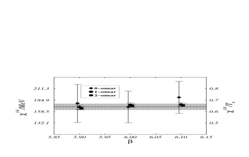
Figure 1: Topological susceptibility in $SU(3)$ pure gauge theory calculated by using 0–, 1– and 2–smeared lattice topological charge operators (see text). The central band indicates the average result and its error bar. Left and right scales are shown in units of MeV and $T_{c}$.

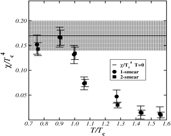
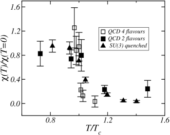
Figure 2: Topological susceptibility in $SU(3)$ pure gauge theory (left) calculated by using 1– and 2–smeared lattice topological charge operators (see text) at finite temperature across the transition at $T_{c}$. The central band indicates the average result at zero temperature as obtained in Fig. 1. A comparison is also made (right) with similar results obtained in full QCD with $N_{f}=2$ and $N_{f}=4$.

4 Recent applications of the field–theoretical method

In the applications of the Pisa method that we have reviewed in Section 3, a determination of $\chi$ was usually needed at several values of the inverse gauge coupling $\beta$, involving several different determinations of the renormalization constants $Z(\beta)$ and $M(\beta)$.

Suppose now that we want to study the behaviour of $\chi(\alpha)$ on some parameter $\alpha$, which does not affect the UV behaviour of the theory, while $\beta$ and other bare parameters (like the masses of dynamical fermions, if present) are kept fixed. This happens in some interesting cases: we will consider the study of the behaviour of $\chi$ across the finite temperature deconfining transition on anisotropic lattices at fixed $\beta$ and variable temporal extension (in this case $\alpha$ is the temporal extent $N_{t}$ of the lattice) and the determination of $\chi$ across the finite density deconfining transition at fixed temperature (in this case $\alpha$ is the chemical potential $\mu$). Renormalization constants are generated by quantum fluctuations at the UV scale, therefore they are independent of $\alpha$ and we can write:

$$\chi(\alpha)=\frac{\chi_{L}(\alpha,\beta)-M(\beta)}{a^{4}(\beta)Z(\beta)^{2}}\;.$$ (12)

In the right hand side of Eq. (12) $\chi_{L}$ is the only quantity which depends on $\alpha$: if one is not interested in an overall multiplicative factor, which is the case when studying the critical behaviour across a phase transition, the determination of a single additive renormalization constant is all that is needed to study the dependence of $\chi$ on $\alpha$. In those cases the field–theoretical method is much simpler and less computer–time consuming than other methods.

4.1 Topology on anisotropic lattices

In the path integral approach to Quantum Field Theory, a finite temperature can be introduced by fixing a finite temporal extent $\tau$ in the Euclidean space–time with (anti)–periodic boundary conditions for (fermionic) bosonic fields, the temperature being $T=1/\tau$. On a lattice this expression becomes $T=1/(N_{t}a(\beta))$. The temperature can thus be varied by changing either the number of lattice sites in the temporal direction or the lattice spacing, hence $\beta$ (we are considering the pure gauge case, otherwise $a$ would depend on the bare quark masses as well). Usually the second option is chosen: indeed for $T$ near the QCD phase transition ($T_{c}\sim 200$ MeV) and for the lattice spacings affordable by present computers ($a^{-1}\sim 1-2$ GeV) typical values of $N_{t}$ are too small to allow a fine tuning of $T$ around $T_{c}$ by only varying the temporal length.

The situation changes when using anisotropic lattices $\!{}^{{\bf?}}$, where different bare couplings are used in temporal and spatial planes, leading to different lattice spacings $a_{s}$ and $a_{t}$. One can thus use a very fine temporal spacing while leaving the spatial ones coarse, with an affordable computer time cost. Anisotropic lattices have been originally introduced to tackle problems related to heavy quarks, glueballs and high temperature thermodynamics which are not easily manageable otherwise. Here we will exploit the possibility of fine tuning $T$ around $T_{c}$ by simply changing $N_{t}$ and leaving $a_{s}$ and $a_{t}$ fixed.

We will consider the pure gauge plaquette action for $N_{c}=3$,

$$S_{G}={\beta\over N_{c}}{1\over\gamma}\sum_{x,i<j\leq 3}\mbox{Re}\mbox{Tr}\left(1-\Pi_{ij}(x)\right)+{\beta\over N_{c}}\gamma\sum_{x,i\leq 3}\mbox{Re}\mbox{Tr}\left(1-\Pi_{i4}(x)\right)\;.$$ (13)

Both $a_{s}$ and $a_{t}$, as well as the renormalized anisotropy $\xi=a_{s}/a_{t}$, are functions of $\beta$ and of the bare anisotropy $\gamma$. Several determinations of those parameters can be found in the literature, we will refer to the following values $\!{}^{{\bf?},{\bf?}}$: $\beta=6.25$, $\gamma=3.2552$, which leads to $\xi=4$ and $a_{s}\approx 0.021$ fm. The critical temperature is reached for $N_{t,c}\approx 35$, so that simulating at a different $N_{t}$ corresponds to $T/T_{c}=N_{t,c}/N_{t}$. We have chosen a spatial lattice size $N_{s}=24$ which corresponds to a spatial extent of about 2 fm.

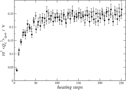
Figure 3: Comparison of the results obtained for $\langle Q_{L}^{2}\rangle_{Q=0}/V$ as a function of the heating steps performed for the operator at the second smearing level on anisotropic lattices of two different temporal extensions: $N_{t}=20$ (circles) and $N_{t}=40$ (triangles) .

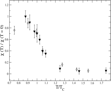
Figure 4: Topological susceptibility as a function of $T/T_{c}$ as obtained on anisotropic lattices by using the operator at the second smearing level (triangles) compared with previous results $\!{}^{{\bf?}}$ obtained using the same operator on isotropic lattice (circles).

We have determined $\chi(T)/\chi(0)$ using the topological charge operator at the second smearing level and compared with previous results obtained on isotropic lattices. As a first step we have checked that the additive renormalization constant is indeed independent of the temporal extent $N_{t}$. We have computed $M$ for two different temporal extensions, $N_{t}=20$ and $N_{t}=40$, corresponding respectively to $T/T_{c}\approx 1.75$ and $T/T_{c}\approx 0.875$. We have obtained $M=(0.249\pm 0.010)\cdot 10^{-5}$ for $N_{t}=20$ and $M=(0.242\pm 0.009)\cdot 10^{-5}$ for $N_{t}=40$, i.e. a very good agreement which is also apparent directly from Fig. 3, where we report $\langle Q^{2}_{L}\rangle_{0}/V$ as a function of the heating step. An average of the two determinations of $M$ has been used for other values of $N_{t}$.

In Fig. 4 we report the quantity $\chi(T)/\chi(0)=(\chi_{L}(T)-M)/(\chi_{L}(0)-M)$ obtained for the 2–smeared operator and compare it with the same quantity determined on isotropic lattices $\!{}^{{\bf?}}$. In the present case $\chi(0)$ is not available and it has been fixed to the value obtained at the lowest available temperature, $T=0.875T_{c}$. A quite good agreement is visible.

4.2 Topology at finite density

An analogous situation is met when varying the chemical potential $\mu$ at constant temperature, which means at fixed $\beta$, $N_{t}$ and quark mass values: indeed a finite $\mu$ does not affect the dynamics at the UV scale, at least until $\mu$ is small with respect to the UV cutoff (for very large values of $\mu$ Pauli blocking sets up with a consequent quenching of fermion dynamics at all scales). We report in this Section results obtained $\!{}^{{\bf?}}$ for the theory with $N_{c}=2$, which is the only case where the sign problem does not make Monte Carlo simulations at finite $\mu$ unfeasible. A lattice of spatial size $N_{s}=14$ and temporal size $N_{t}=6$ has been used, with dynamical staggered fermions corresponding to 8 continuum degenerate flavours of bare mass $am=0.07$ and an inverse coupling $\beta=1.5$, corresponding to a temperature well below $T_{c}$: a phase transition to deconfined matter is therefore expected after increasing $\mu$ beyond some critical value $\mu_{c}$. The aim was to investigate the fate of topological excitations, hence of $\chi$, across the finite density phase transition.

In the l.h.s. of Fig. 5 the estimates of $M$ obtained for four different values of $\mu$ are shown. They look compatible within errors as they should be if the renormalization procedure is correct and no density effects are introduced into the subtractions. Hence also in this case a single renormalization constant is enough to determine the ratio $\chi(\mu)/\chi(0)=(\chi_{L}(\mu)-M)/(\chi_{L}(0)-M)$ which is displayed in the r.h.s. of Fig. 5. It shows a clear drop at a critical value $\mu_{c}$, analogously to what happens for the finite temperature phase transition.

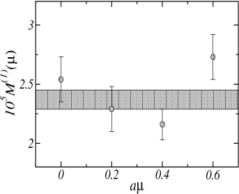
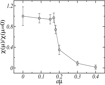
Figure 5: Additive renormalization (left) and $\chi(\mu)/\chi(0)$ (right) as a function of $a\mu$ for the theory at finite density with 2 colours and 8 continuum dynamical flavours.

References

References

- [1] E. Witten, Nucl. Phys. B 156, 269 (1979).
- [2] G. Veneziano, Nucl. Phys. B 159, 213 (1979).
- [3] E. Shuryak, Comments Nucl. Part. Phys. 21, 235 (1994).
- [4] M. Marchi and E. Meggiolaro, Nucl. Phys. B 665, 425 (2003).
- [5] P. Costa et al., Phys. Rev. D 70, 116013 (2004).
- [6] P. Di Vecchia, K. Fabricius, G. C. Rossi, and G. Veneziano, Nucl. Phys. B 192, 392 (1981).
- [7] M. Campostrini, A. Di Giacomo and H. Panagopoulos, Phys. Lett. B 212, 206 (1988).
- [8] B. Allés and E. Vicari, Phys. Lett. B 268, 241 (1991).
- [9] E. Seiler and I. O. Stamatescu, preprint MPI–PAE/PTh 10/87 (1987), unpublished.
- [10] K. Osterwalder in “Constructive Field Theory”, Lecture Notes in Physics, no 25 (1973), edited by G. Velo and A. S. Wightman.
- [11] P. Menotti and A. Pelissetto, Nucl. Phys. Proc. Suppl. 4, 644 (1988).
- [12] B. Allés, M. D’Elia, A. Di Giacomo and R. Kirchner, Phys. Rev. D 58, 114506 (1998).
- [13] I. Horváth et al., Phys. Lett. B 617, 49 (2005).
- [14] E.–M. Ilgenfritz, K. Koller, Y. Koma, G. Schierholz, T. Streuer and V. Weinberg, hep–lat/0512005.
- [15] M. Lüscher, Comm. Math. Phys. 85, 39 (1982).
- [16] P. Woit, Phys. Rev. Lett. 51, 638 (1983).
- [17] E.–M. Ilgenfritz, M. L. Laursen, G. Schierholz, M. Müller–Preussker and H. Schiller, Nucl. Phys. B 268, 693 (1986).
- [18] M. Teper, Phys. Lett. B 171, 86 (1986).
- [19] J. Smit and C. Vink, Nucl. Phys. B 286, 485 (1987).
- [20] M. Campostrini, A. Di Giacomo H. Panagopoulos and E. Vicari, Nucl. Phys. B 329, 683 (1990).
- [21] A. Di Giacomo and E. Vicari, Phys. Lett. B 275, 429 (1992).
- [22] B. Allés, M. Campostrini, A. Di Giacomo, Y. Gündüç and E. Vicari, Phys. Rev. D 48, 2284 (1993).
- [23] B. Allés, G. Boyd, M. D’Elia, A. Di Giacomo and E. Vicari, Phys. Lett. B 389, 107 (1996).
- [24] B. Allés et al., Phys. Rev. D 58, 071503 (1998).
- [25] F. Farchioni and A. Papa, Nucl. Phys. B 431, 686 (1994).
- [26] P. H. Ginsparg and K. G. Wilson, Phys. Rev. D 25, 2649 (1982).
- [27] H. Neuberger, Phys. Lett. B 417, 141 (1998).
- [28] M. Lüscher, Phys. Lett. B 428, 342 (1998).
- [29] B. Allés, M. D’Elia, A. Di Giacomo and C. Pica, Pro. Sci. LAT2005, 316 (2005), hep–lat/0509024 and work in progress.
- [30] M. D’Elia, Nucl. Phys. B 661, 139 (2003).
- [31] C. Christou, A. Di Giacomo, H. Panagopoulos and E. Vicari, Phys. Rev. D 53, 2619 (1996).
- [32] B. Allés, M. D’Elia and A. Di Giacomo, Phys. Lett. B 412, 119 (1997).
- [33] B. Allés, M. D’Elia and A. Di Giacomo, Nucl. Phys. B 494, 281 (1997).
- [34] G. Boyd et al., Nucl. Phys. B 469, 419 (1996).
- [35] B. Lucini, M. Teper and U. Wenger, JHEP 0401:061 (2004).
- [36] B. Allés, M. D’Elia and A. Di Giacomo, Phys. Lett. B 483, 139 (2000).
- [37] D. Espriu and R. Tarrach, Z. Phys. C 16, 77 (1982).
- [38] B. Allés, A. Di Giacomo, H. Panagopoulos and E. Vicari, Phys. Lett. B 350, 70 (1995).
- [39] C. Vafa and E. Witten, Phys. Rev. Lett. 53, 535 (1984).
- [40] B. Allés, M. D’Elia and A. Di Giacomo, Phys. Rev. D 71, 034503 (2005).
- [41] T.R. Klassen, Nucl. Phys. B 533, 557 (1998).
- [42] N. Ishii, H. Suganuma and H. Matsufuru, Phys. Rev. D 66, 114507 (2002).
- [43] B. Allés, M. D’Elia, M.P. Lombardo and M. Pepe, Nucl. Phys. Proc. Suppl. 94, 441 (2001); B. Allés, M. D’Elia and M.P. Lombardo, hep–lat/0602022.