MPP-2006-1

January 2006

Repairing Stevenson’s step in the $4d$ Ising model

Janos Balog

Research Institute for Particle and Nuclear Physics

1525 Budapest 114, Pf. 49, Hungary

Ferenc Niedermayer^∗

Institute for Theoretical Physics, University of Bern

CH-3012 Bern, Switzerland

Peter Weisz

Max-Planck-Institut für Physik

Föhringer Ring 6, D-80805 München, Germany

Abstract

In a recent paper Stevenson claimed that analysis of the data on the wave function renormalization constant near the critical point of the $4d$ Ising model is not consistent with analytical expectations. Here we present data with improved statistics and show that the results are indeed consistent with conventional wisdom once one takes into account the uncertainty of lattice artifacts in the analytical computations.

—————
^∗On leave from Eötvös University, HAS Research Group, Budapest, Hungary

1 Introduction

One of the apparently simplest quantum field theories in four dimensions is the $\phi^{4}$ theory with $n$ components. Conventional wisdom (CW) holds that the theory is trivial for all $n\geq 1$ . Unfortunately there is presently no rigorous proof. One relies heavily on the validity of renormalization group (RG) equations for physical quantities [?] together with boundary conditions at finite cutoff provided by non-perturbative methods [?,?].

Apart from its purely theoretical interest it is of phenomenological relevance since for the case $n=4$ it constitutes the pure Higgs sector of the Minimal Standard Model (MSM). The fact that $\phi^{4}_{4}$ is (probably) trivial does not invalidate (renormalized) perturbative computations for amplitudes at energies well below the physical cutoff where the MSM may be a good effective theory.

In the past triviality has been invoked to propose upper bounds on the mass of the Higgs boson (see e.g. refs. [?–?]). It must be stressed that these bounds are non-universal, they depend on the particular regularization. But for a given regularization it is conventionally accepted that such a bound can be given a precise meaning. In recent papers Cea, Cosmai, and Consoli (CCC) [?,?] claim that triviality itself cannot be used to place upper bounds on the Higgs mass even for a given regularization. They assert that standard predictions of the RG analysis for the behavior of some quantities near the critical line are not valid. If true this would indeed be rather important because it would reveal a serious flaw in our conventional theoretical understanding of the pure $\phi^{4}_{4}$!

In ref. [?] Duncan, Willey and the present authors explained why critiques of the standard picture raised in ref. [?] were not relevant. Nevertheless one must admit that the unconventional picture of CCC cannot be ruled out by present numerical simulations. Recently two papers appeared, the first by CCC [?] and the second by Stevenson [?], again claiming finer but significant discrepancies between quantitative (standard) analytic predictions and numerical data in the $4d$ Ising model.

It is the purpose of this paper to reply to these challenges and to demonstrate that they are too weak to seriously cast doubt on CW. The main objection by CCC and one by Stevenson are rather easy to dismiss. A second objection by Stevenson is more difficult. It concerns a certain difference $\triangle$ between the wave function renormalization constants below and above the critical point

$$\triangle=\widehat{Z_{{\hbox{\sixrm R}}}}(\kappa=0.074)-\widehat{Z_{{\hbox{\sixrm R}}}}(\kappa=0.0751)\,,$$ (1.1)

which we have called “Stevenson’s step” in the title. The $\kappa$ values chosen here are about the closest to the critical point where one can presently obtain good statistics with some (but not unreasonable) computational effort . Stevenson claims that “theoretical predictions for $\triangle$ cannot be pushed above $0.05$ well short of the “experimental” value $\triangle_{\rm MC}=0.071(6)$”. It is of course debatable whether such a small discrepancy indicates a potential problem, however we decided it merited more careful investigation.

It is however clear that one is here addressing few percent effects, and to clarify the situation we need both data and analyses which are precise to this level. The main analytic sources of error concern the treatment of higher order cutoff effects in the framework of renormalized PT. The main sources of error in the numerical side are the determinations of the zero momentum mass $m_{{\hbox{\sixrm R}}}$; apart from the statistical errors one has the systematic errors in the procedures to extract $m_{{\hbox{\sixrm R}}}$ from the (finite volume) data particularly in the symmetry broken phase.

In the next section we present a summary of the available raw data in both the symmetric and broken phases. We have performed simulations in both phases and in particular increased the statistics at previously measured $\kappa$ values in the broken phase by a factor of $\sim 10$.

We then discuss various determinations of $\widehat{Z_{{\hbox{\sixrm R}}}}$ from the data and compare with theoretical expectations. Next we show that these data are not in contradiction with conventional wisdom. The reason for this conclusion differing from that of Stevenson has two main origins. Firstly unfortunately our central value of $\widehat{Z_{{\hbox{\sixrm R}}}}$ at $\kappa=0.0751$ in [?] is about one standard deviation lower than that obtained from the present run. In this connection we remark that in those runs we were not aiming at high precision but only sufficient to reach our goal to present evidence that $\widehat{Z_{{\hbox{\sixrm R}}}}$ is not increasing logarithmically as one approaches $\kappa_{\rm c}$. Secondly we point out that there is a quantitative uncertainty on the ${\rm O}(a^{2})$ lattice artifacts which are of course increasingly relevant as one goes away from the critical point. This is of course not at all new, however sometimes forgotten and perhaps underestimated in standard RG analyses.

2 Ising MC simulation and results

We work on hypercubic lattices of volume $L^{4}$ with periodic boundary conditions in each direction and with standard action. In this paper we adopt the notations and definitions in ref. [?], and will generally not repeat them here.

If one just wanted to obtain Stevenson’s step, measurements at only two $\kappa$ values are required. However precise simulations at these points are CPU expensive and hence it is useful to compute also at points with smaller correlation length to observe the approach to Stevenson’s chosen points which hopefully also reflects the approach to the critical point. As mentioned above we have simulated in both phases. In the symmetric phase this served as a check with respect to previous simulation results by other authors. In Table 1 we collect the (to our knowledge) best data for observables in the symmetric phase, which are obtained without a fitting procedure; by “best” we mean data with the largest statistics and for lattices with large physical volumes $mL\gtrsim 6$. (Our tables can be found in Appendix B.) All the values in this table are from the present simulation except those for $\kappa=0.07102$ which come from ref. [?]. The previous results of Montvay, Münster and Wolff [?] for their lattices A,C ($\kappa=0.071,L=12$ and $\kappa=0.0732,L=20$) are in complete agreement with ours, but have larger errors. Note that we have also measured at a new point $\kappa=0.07436$ slightly closer to $\kappa_{\rm c}$ than previous ones.

Also included in Table 1 is the quantity

$$m_{{\hbox{\sixrm R}}}^{\rm naive}\equiv\sqrt{\frac{\widehat{k_{0}}^{2}\widetilde{G}(k_{0})}{\widetilde{G}(0)-\widetilde{G}(k_{0})}}\,,\,\,\,\,k_{0}=\left(\frac{2\pi}{L},0,0,0\right)\,,$$ (2.2)

where $\widetilde{G}$ is the Fourier transform of the (connected) two–point function. $m_{{\hbox{\sixrm R}}}^{\rm naive}$ tends to the desired zero momentum mass in the infinite volume limit .

In Table 2 we present a similar data collection for the broken phase. This is an update of Table 3 in [?]; here we have increased our statistics by a factor of $\sim 10$. In these runs we also measured the connected 3–point function $\chi_{3}$ (except for one lattice). For a large subset of the runs in the broken phase we also measured the correlation matrix of the time slice field $\varphi(t)$ with the composite field

$$\varphi_{2}(t)\propto\varphi(t)^{2}\,,\,\,\,\,\varphi(t)=\sum_{\bf x}\phi(t,{\bf x})\,.$$ (2.3)

3 Determination of $m_{{\hbox{\sixrm R}}}$ and derived quantities

The usual expressions for the wave function renormalization constant and renormalized couplings involve the infinite volume zero momentum mass. In particular a precise determination of $\widehat{Z_{{\hbox{\sixrm R}}}}$ (as required to discuss Stevenson’s step) requires an equally reliable determination of $m_{{\hbox{\sixrm R}}}$. Firstly in considering the $r$–point functions one can verify using the formulae given in ref. [?] that finite volume effects coming from tunneling are negligible for our lattices. We then adopted two fitting procedures.

In the first we made fits of $\widetilde{G}(k)^{-1}$ for $k=\left(2\pi s/L,0,0,0)\right)$ for small values of $s$ ($s\leq 3$ in the symmetric phase and $s\leq 4$ in the broken phase) to polynomials in $\widehat{k}^{2}$ and just recorded good fits with $\chi^{2}/{\rm dof}<1$.

Due to the discreteness of available values of $k$ the determination of the slope at $k=0$ is prone to discretization error. A removal of this deficit is attempted in a second procedure where we performed fits of the connected (time slice) correlation function $S(t)$ to obtain the physical mass $m$. Relying on the expectation that finite volume effects on $m$ are extremely small in this model when $mL>7$, we obtain an estimate for the infinite volume $m_{{\hbox{\sixrm R}}}$ by computing the second moment with the data in a large portion of the lattice volume and then computing the contribution from the rest of the (infinite) volume using the measurement of $m$.

Our fits of $S(t)$ were in terms of one and two mass cosh functions; for the $1-$mass case we fitted only distances $t>1/m$ and for the $2-$mass case $t\gtrsim 2/3m$. The $2-$mass fits were constrained to have the second mass fixed to $3m$ for the symmetric phase and $2m$ for the broken phase. The $2-$mass fits give (as expected) a slightly lower central value of $m$ but a slightly larger error than the $1-$mass fit. This is again reflected in the resulting values for $m_{{\hbox{\sixrm R}}}$ and $\widehat{Z_{{\hbox{\sixrm R}}}}$. Figs. 1, 2 are typical examples in the symmetric and broken phases respectively, which illustrate the good quality of the fits and the relatively very small contribution of the higher particle states.

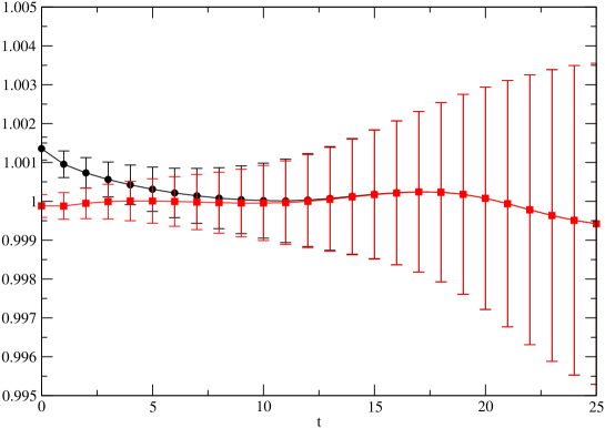
Figure 1: Ratio of the measured $S(t)$ to the $1-$ and $2-$mass contributions (filled circles and squares respectively) to the $2-$mass fit for the $\kappa=0.0744,L=52$ lattice.

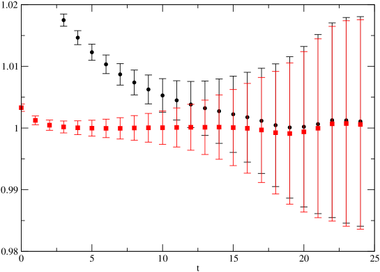
Figure 2: As for Fig. 1 but for the $\kappa=0.0751,L=48$ lattice.

For the subset of data in the broken phase where we had the full correlation matrix mentioned above we found that the two operators $\varphi,\varphi_{2}$ were nearly parallel, both coupling very weakly to the 2–particle state, and thus this did not help to significantly reduce the errors on $m$.

In Tables 3 and 4 we give results for $m$ and quantities derived from various estimates of $m_{{\hbox{\sixrm R}}}$ in the symmetric and broken phase respectively. In practically all cases all methods to determine $m_{{\hbox{\sixrm R}}}$ gave compatible results .

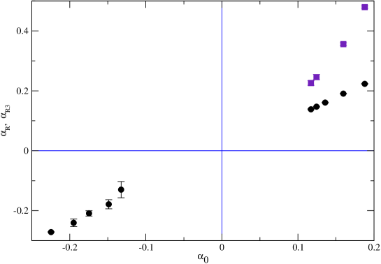
Figure 3: Renormalized couplings versus $\alpha_{0}$; $\alpha_{0}<0$ corresponds to the symmetric phase and $\alpha_{0}>0$ to the broken phase. Full circles and squares represent $\alpha_{{\hbox{\sixrm R}}}$ and ${\alpha_{{\hbox{\sixrm R}}}}_{3}$, respectively. For $\alpha_{0}<0$ we have plotted $-\alpha_{{\hbox{\sixrm R}}}$.

In Fig. 3 we plot renormalized couplings ($\alpha_{{\hbox{\sixrm R}}}=g_{{\hbox{\sixrm R}}}/(16\pi^{2})$) in the symmetric and broken phases using $m_{{\hbox{\sixrm R}}}=m_{{\hbox{\sixrm R}}}^{\rm naive}$ versus

$$\alpha_{0}(\kappa)\equiv\frac{2\,{\rm sign}(\tau)}{3\ln|\tau|}\,,\,\,\,\,\,\,\,\,\tau=1-\frac{\kappa}{\kappa_{\rm c}}\,,$$ (3.4)

with the presently best estimate of $\kappa_{\rm c}=0.074848$ from ref. [?]. In the symmetric phase the coupling is defined through the connected 4–point function. In the broken phase we have included the renormalized coupling $g_{{\hbox{\sixrm R}}}$ defined through the vacuum expectation value and another coupling $g_{{\hbox{\sixrm R}}3}$ defined through the connected 3–point function. According to standard RG analysis these should behave as $16\pi^{2}|\alpha_{0}|$ as $\tau\to 0$. Note that the relations of the measured values for $g_{{\hbox{\sixrm R}}}$ and $g_{{\hbox{\sixrm R}}3}$ are quite consistent with those obtained in renormalized perturbation theory:

$$g_{{\hbox{\sixrm R}}3}=g_{{\hbox{\sixrm R}}}\left(1+3\alpha_{{\hbox{\sixrm R}}}+3.75\alpha_{{\hbox{\sixrm R}}}^{2}+\dots\right)\,.$$ (3.5)

3.1 Stevenson’s step

Stevenson presents plots with respect to $\kappa$ whereas we prefer to present plots wrt $\alpha_{0}$ since dependence of quantities of interest on this variable are expected to be smoother. In Fig. 4 we plot $\widehat{Z_{{\hbox{\sixrm R}}}}$ obtained using $m_{{\hbox{\sixrm R}}}$ values obtained from the 1-mass fit method. Using $m_{{\hbox{\sixrm R}}}=m_{{\hbox{\sixrm R}}}^{\rm naive}$ or $m_{{\hbox{\sixrm R}}}$ corresponding to the 2-mass fit method would result in very similar plots, with somewhat larger errors for the latter case. (The same applies also to Fig. 5.) Here one certainly does not see any signal of a discontinuity at the critical point.

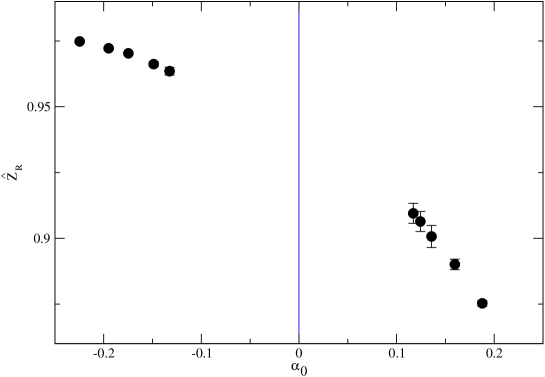
Figure 4: Measured values of $\widehat{Z_{{\hbox{\sixrm R}}}}$ using $m_{{\hbox{\sixrm R}}}$ obtained by the 1-mass fit method.

As mentioned above the value of $\widehat{Z_{{\hbox{\sixrm R}}}}(\kappa=0.0751)$ cited in [?] is over one standard deviation away from our present value . For Stevenson’s step we would now quote a measured value of

$$\triangle_{\rm MC}=0.057(6)\,.$$ (3.6)

Given the more precise value of $\widehat{Z_{{\hbox{\sixrm R}}}}$ at $\kappa=0.0751$ Stevenson may not have written his paper. On the other hand this new value for $\triangle$ is still bigger than what Stevenson calls analytically feasible. We however disagree with this opinion. The problem is that our quantitative control of ${\rm O}(a^{2})$ effects in the RG equations is not sufficient. Although these are rather small at the values of $\kappa$ used in the definition of $\triangle$, they are still not negligible when discussing possible discrepancies between theory and “experiment”. In refs. [?,?] some such effects were taken into account by including the $m_{{\hbox{\sixrm R}}}$ dependence of perturbative RG coefficients appearing at low orders of perturbation theory. This procedure was also adopted by Stevenson [?]. It is however just a pragmatic procedure (i.e. practically the best one could quantitatively do at the time), but it is not a quantitatively systematic prescription. Firstly it is not consistent to include ${\rm O}(a^{2})$ effects while ignoring higher perturbative effects . Secondly even if one disregards this, the leading ${\rm O}(m_{{\hbox{\sixrm R}}}^{2})$ effects at $r$–loop order are of generically of the form $g_{{\hbox{\sixrm R}}}^{c+r}m_{{\hbox{\sixrm R}}}^{2}|\ln m_{{\hbox{\sixrm R}}}|^{r}$ and hence all quantitatively of the same order since the RG equations predict $g_{{\hbox{\sixrm R}}}\sim 1/\ln m_{{\hbox{\sixrm R}}}$.

To obtain the leading cutoff effects one must follow the method of Symanzik [?]. The analysis shows that the leading artifacts for the correlation functions (for the case $n=1$) are of the form

$$\Gamma\sim\Gamma^{(0)}+{\rm O}\left(m_{{\hbox{\sixrm R}}}^{2}|\ln m_{{\hbox{\sixrm R}}}|^{1/3}\right).$$ (3.7)

Here $\Gamma^{(0)}$ is the formal perturbative sum; in the process of defining this non-perturbatively it could be that renormalon-type effects would lead to cutoff effects of the same form as the leading operator insertion. But even though the form of the leading cutoff corrections may be known the amplitude is undetermined.

Another simple exercise to appreciate this point is to compute in the leading order of the $1/n$ expansion. In that limit the cutoff effects are of the order $m_{{\hbox{\sixrm R}}}^{2}$ however these are not given by taking the limit $n\to\infty$ of the first perturbative contributions. Some illustrations are given in Appendix A.

Having realized that we have unfortunately insufficient quantitative knowledge of $m_{{\hbox{\sixrm R}}}^{2}$–effects it is still legitimate to ask if the numerically found value of $\triangle$ looks inconsistent with the conventional theoretical expectation that $\widehat{Z_{{\hbox{\sixrm R}}}}$ approaches the same value $\widehat{C}_{2}$ coming from both sides of the critical point:

$${\rm CW}:\,\,\,\,\,\lim_{\kappa\to\kappa_{\rm c}^{+}}\widehat{Z_{{\hbox{\sixrm R}}}}=\widehat{C}_{2}=\lim_{\kappa\to\kappa_{\rm c}^{-}}\widehat{Z_{{\hbox{\sixrm R}}}}\,,\,\,\,\,\widehat{C}_{2}=2\kappa_{\rm c}C_{2}\,.$$ (3.8)

To illustrate the situation we consider two expressions $\widehat{C}_{2}^{(I)}$ and $\widehat{C}_{2}^{(II)}$ which we would eventually expect to approach $\widehat{C}_{2}$ faster than $\widehat{Z_{{\hbox{\sixrm R}}}}$. The first, which arises in the renormalization scheme of [?] is defined by dividing $\widehat{Z_{{\hbox{\sixrm R}}}}$ by its perturbative expansion truncated at 2–loops:

$$\widehat{C}_{2}^{(I)}\equiv\left\{\begin{split}&\widehat{Z_{{\hbox{\sixrm R}}}}\left(1+\frac{1}{18}\alpha_{{\hbox{\sixrm R}}}+0.100896\alpha_{{\hbox{\sixrm R}}}^{2}\right)^{-1}\,,\,\,\,\,\,\,{\rm for}\,\,\kappa<\kappa_{\rm c}\,,\\ &\widehat{Z_{{\hbox{\sixrm R}}}}\left(1-\frac{7}{36}\alpha_{{\hbox{\sixrm R}}}-0.538874\alpha_{{\hbox{\sixrm R}}}^{2}\right)^{-1}\,,\,\,\,\,\,\,{\rm for}\,\,\kappa>\kappa_{\rm c}\,.\\ \end{split}\right.$$ (3.9)

The second, which is a natural choice in a field theoretical context, is merely defined from the first by

$$\widehat{C}_{2}^{(II)}\equiv\frac{\kappa}{\kappa_{\rm c}}\widehat{C}_{2}^{(I)}\,.$$ (3.10)

The difference between the two functions is just an order $m_{{\hbox{\sixrm R}}}^{2}$ cutoff effect [?,?]:

$$\kappa_{\rm c}-\kappa = \phantom{\frac{1}{2}}C_{3}m_{{\hbox{\sixrm R}}}^{2}g_{{\hbox{\sixrm R}}}^{-1/3}\left\{1+{\rm O}(g_{{\hbox{\sixrm R}}})\right\}\,,\,\,\,\,{\rm for}\,\,\kappa<\kappa_{\rm c}\,,$$ (3.11)

$$\kappa-\kappa_{\rm c} = \frac{1}{2}C^{\prime}_{3}m_{{\hbox{\sixrm R}}}^{2}g_{{\hbox{\sixrm R}}}^{-1/3}\left\{1+{\rm O}(g_{{\hbox{\sixrm R}}})\right\}\,,\,\,\,\,{\rm for}\,\,\kappa>\kappa_{\rm c}\,,$$ (3.12)

which incidentally has the same cutoff effects as in (3.7). In Fig. 5 we plot them together to give an idea on the importance of the ${\rm O}(m_{{\hbox{\sixrm R}}}^{2})$ effects. Both are certainly not inconsistent with the expectation that the limits are the same on both sides (note the difference in scales on the vertical axis). Indeed if one allowed to naively

Figure 5: Top, $C_{2}^{(I)}$ (renormalization scheme of refs. [2,3]). Bottom, $C_{2}^{(II)}$ (field theoretical renormalization scheme). Note the different vertical scales.

extrapolate the curves by eye one would probably infer a different sign for the difference of the limiting values from the two plots.

If one had much more precise data one could attempt constrained fits to the CW but this is not warranted with the present data. Assuming CW we would now quote $\widehat{C}_{2}=0.95(1)$ which corresponds to $\ln C_{2}=1.85(1)$ to be compared with the result $\ln C_{2}=1.87(1)$ in [?].

4 Reply to some other critiques

In ref. [?] the authors reconsider the quantity $v^{2}\chi$ in the broken phase which according to CW behaves as

$$v^{2}\chi=a_{1}\left(\ell-\frac{25}{27}\ln\ell\right)+a_{2}+\dots\,,$$ (4.13)

where $\ell\equiv|\ln(\kappa-\kappa_{\rm c})|$ with

$$a_{1} = \frac{9C_{2}^{2}}{32\pi^{2}}\,,$$ (4.14)

$$\frac{a_{2}}{a_{1}} = \ln C^{\prime}_{3}+2\ln C^{\prime}_{1}-1.6317\,.$$ (4.15)

A fit of the expression (4.13) to the data gave [?] $a_{1}=1.267(14)$ and $a_{2}=-2.89(8)$ whereas the theoretical prediction based on the results quoted in [?] for the values of the non-perturbative constants $C_{1}$, $C_{2}$ and $C_{3}$ is $a_{1}=1.20(3)$ and $a_{2}=-1.6(5)$. The authors of  [?] claim that such a comparison “shows that the quality of the 2-loop fit is poor”. How they can reach such a conclusion is surprising to us. Firstly the values $a_{1}$ agree within one standard deviation. Secondly the value of $a_{2}$ from the fits can only be regarded as effective. Higher order terms e.g. of the form $1/\ell$ are completely neglected in the fit.

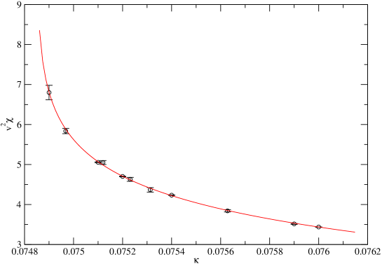
Figure 6: 2-parameter fit of the expression (4.13) to the data from Table 2.

We have made new fits including all data from Table 2, omitting only the $\kappa>0.076$ lattices and the one corresponding to $\kappa=0.07504$ (because of its too small physical volume). Our first fit, which is shown in Fig. 6, has an acceptable $\chi^{2}/{\rm dof}=1.2$ and yields

$$a_{1}=1.224(6)\qquad\qquad{\rm and}\qquad\qquad a_{2}=-2.68(3).$$ (4.16)

As discussed at the end of the previous section, our $\widehat{Z_{{\hbox{\sixrm R}}}}$ data prefer a slightly smaller $C_{2}$ value corresponding to $\ln C_{2}=1.85(1)$. This changes the theoretical prediction to $a_{1}=1.15(3)$. We have made a second two-parameter fit with a third term of the form $a_{3}/\ell$ added but where the first coefficient was kept fixed at $a_{1}=1.15$. The result of this fit is

$$a_{1}=1.15,\qquad a_{2}=-1.80(3),\qquad a_{3}=-3.5(2),\qquad\chi^{2}/{\rm dof}=1.0.$$ (4.17)

The fact that it is impossible to distinguish between (4.16) and (4.17) illustrates the point we made in the previous paragraph. Taking into account all the uncertainties we find the agreement between theory and MC ‘experiment’ satisfactory.

We completely disagree with the implications of Section 5 in ref. [?]. Here Stevenson proposes that a proper extraction of $m_{{\hbox{\sixrm R}}}$ is obtained by globally fitting the data for $\widetilde{G}(k)^{-1}$ in the whole available momentum range to the form of the free lattice propagator with standard (nearest neighbor) action. But this is an a priori incorrect procedure since $m_{{\hbox{\sixrm R}}}$ must be extracted from data including only low momenta. Accepting this fact it is then a rather surprising “experimental” finding that the numerically measured propagator is so extremely close to the naive propagator; only a detailed look reveals that there is some significant deviation at larger momenta. It is a bit easier to see the deviation in coordinate space e.g. in Fig. 7 we plot the effective masses at $\kappa=0.0751$. The effective mass $m_{\mathrm{eff}}(t+0.5)$ is defined for the 1–mass case by $m_{1}$ in the ansatz $B\left[\exp(-m_{1}t^{\prime})+\exp(-m_{1}(L-t^{\prime}))\right]$ with the parameters defined from $S(t^{\prime})$ at $t^{\prime}=t,t+1$. This would be constant for a free standard lattice propagator, but the data shows clear $t$-dependence. For the constrained 2–mass fit $\sum_{i=1}^{2}B_{i}\left[\exp(-m_{i}t^{\prime})+\exp(-m_{i}(L-t^{\prime}))\right]$ with $m_{2}=2m_{1}$, $m_{\mathrm{eff}}(t)=m_{1}$ from the correlation function at $t^{\prime}=t-1,t,t+1$.

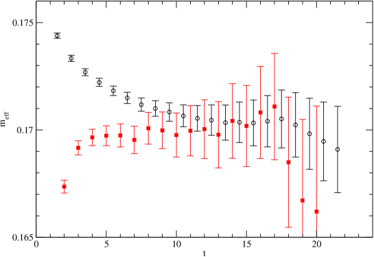
Figure 7: Effective masses for the $\kappa=0.0751,L=48$ lattice. The circles are from the 1-mass definition, and the squares from the 2-mass fit definition as described in the text.

5 Conclusions

An experimental observation contradicting a prediction of an until then accepted theory is always an exciting event. It invalidates the theory as it stands and inevitably leads to progress in our understanding. Similarly finding mismatches between theoretical predictions and numerical simulations in the $\phi^{4}_{4}$ theory as claimed in refs. [?,?] would be a serious blow if they withheld scrutiny. We hope to have convinced the reader in this paper that conventional wisdom concerning this structurally simple theory is still alive. Although present numerical simulations support CW, the scenario can unfortunately only be “nailed down” by analytic proofs.

5.1 Acknowledgments

We thank the Leibniz-Rechenzentrum where part of the computations were carried out. This investigation was supported in part by the Hungarian National Science Fund OTKA (under T049495 and T043159) and by the Schweizerischer Nationalfonds.

Appendix Appendix A: leading order $1/n$ expansion

For the $n$-component model we take over the notations of ref. [?]. In the $1/n$ expansion one takes $n\to\infty$ with

$${\widehat{\lambda}}\equiv n\lambda$$ (A.18)

held fixed.

In the symmetric phase in leading order we have

$$\widehat{Z_{{\hbox{\sixrm R}}}}=1\,,$$ (A.19)

and given ${\widehat{\lambda}},\kappa<\kappa_{\rm c}=\frac{1}{2}J_{1}(0)$ the renormalized zero momentum mass $m_{{\hbox{\sixrm R}}}$ is determined by

$$\frac{\kappa^{2}}{{\widehat{\lambda}}}\left(m_{{\hbox{\sixrm R}}}^{2}+8-\frac{1}{\kappa}\right)+2\kappa-J_{1}(m_{{\hbox{\sixrm R}}})=0\,,$$ (A.20)

where (see ref. [?])

$$J_{q}(m_{{\hbox{\sixrm R}}})=\int_{-\pi}^{\pi}\frac{{\rm d}^{4}k}{(2\pi)^{4}}\left(\hat{k}^{2}+m_{{\hbox{\sixrm R}}}^{2}\right)^{-q}\,.$$ (A.21)

The renormalized coupling $\widehat{g_{{\hbox{\sixrm R}}}}\equiv ng_{{\hbox{\sixrm R}}}$ is given by

$$\widehat{g_{{\hbox{\sixrm R}}}}=\frac{6}{\frac{\kappa^{2}}{{\widehat{\lambda}}}+J_{2}(m_{{\hbox{\sixrm R}}})}\,.$$ (A.22)

For ${\widehat{\lambda}}=\infty$ there is a simplification and

$$m_{{\hbox{\sixrm R}}}\frac{\partial\widehat{g_{{\hbox{\sixrm R}}}}}{\partial m_{{\hbox{\sixrm R}}}} = \frac{24m_{{\hbox{\sixrm R}}}^{2}J_{3}(m_{{\hbox{\sixrm R}}})}{J_{2}(m_{{\hbox{\sixrm R}}})^{2}}$$ (A.23)

$$= \frac{s_{1}}{3}\widehat{g_{{\hbox{\sixrm R}}}}^{2}+m_{{\hbox{\sixrm R}}}^{2}B_{1}(m_{{\hbox{\sixrm R}}})\,,$$ (A.24)

with $s_{1}=1/(16\pi^{2})$ and

$$B_{1}(m_{{\hbox{\sixrm R}}})=\frac{24\left(J_{3}(m_{{\hbox{\sixrm R}}})-\frac{s_{1}}{2m_{{\hbox{\sixrm R}}}^{2}}\right)}{J_{2}(m_{{\hbox{\sixrm R}}})^{2}}\,.$$ (A.25)

With the expansions of $J_{q}(m_{{\hbox{\sixrm R}}})$ in [?] for small $m_{{\hbox{\sixrm R}}}$ the non-scaling piece behaves as

$$B_{1}(m_{{\hbox{\sixrm R}}})\sim-\frac{3}{s_{1}\ln(m_{{\hbox{\sixrm R}}}^{2})}+\dots$$ (A.26)

In renormalized PT one obtains (in the limit $n\to\infty$):

$$m_{{\hbox{\sixrm R}}}\frac{\partial\widehat{g_{{\hbox{\sixrm R}}}}}{\partial m_{{\hbox{\sixrm R}}}}=\frac{4m_{{\hbox{\sixrm R}}}^{2}}{8+m_{{\hbox{\sixrm R}}}^{2}}\widehat{g_{{\hbox{\sixrm R}}}}+\widehat{g_{{\hbox{\sixrm R}}}}^{2}\left(\frac{s_{1}}{3}+\frac{2m_{{\hbox{\sixrm R}}}^{2}}{3}\left[J_{3}(m_{{\hbox{\sixrm R}}})-\frac{J_{1}(m_{{\hbox{\sixrm R}}})}{(8+m_{{\hbox{\sixrm R}}}^{2})^{2}}\right]\right)+{\rm O}(\widehat{g_{{\hbox{\sixrm R}}}}^{3}m_{{\hbox{\sixrm R}}}^{2})\,.$$ (A.27)

So including the leading non-scaling effects we write

$$m_{{\hbox{\sixrm R}}}\frac{\partial\widehat{g_{{\hbox{\sixrm R}}}}}{\partial m_{{\hbox{\sixrm R}}}}=\frac{s_{1}}{3}\widehat{g_{{\hbox{\sixrm R}}}}^{2}+\frac{m_{{\hbox{\sixrm R}}}^{2}}{\ln(m_{{\hbox{\sixrm R}}}^{2})}\sum_{s=0}f_{s}+{\rm O}(m_{{\hbox{\sixrm R}}}^{2}/\ln^{2}m_{{\hbox{\sixrm R}}}^{2})$$ (A.28)

where $f_{s}$ denotes the coefficient from the $s$ loops. For the first coefficients we have

$$f_{0}=-\frac{3}{s_{1}}\,,\,\,\,\,f_{1}=-\frac{3}{s_{1}}\,,$$ (A.29)

to be compared to the non-perturbative result in Eq. (A.26).

Although $\widehat{Z_{{\hbox{\sixrm R}}}}$ is so simple, the $\gamma$–function defined in [?] is not zero e.g. in the limit ${\widehat{\lambda}}\to\infty$:

$$v\equiv\frac{1}{2}m_{{\hbox{\sixrm R}}}\frac{\partial}{\partial m_{{\hbox{\sixrm R}}}}\ln Z_{{\hbox{\sixrm R}}}=m_{{\hbox{\sixrm R}}}^{2}\frac{J_{2}(m_{{\hbox{\sixrm R}}})}{J_{1}(m_{{\hbox{\sixrm R}}})}\,,\,\,\,\,\,\,\,\,\,({\widehat{\lambda}}=\infty)\,.$$ (A.30)

For small $m_{{\hbox{\sixrm R}}}$ we have

$$v\sim-\frac{s_{1}}{J_{1}(0)}m_{{\hbox{\sixrm R}}}^{2}\ln(m_{{\hbox{\sixrm R}}}^{2})+\dots$$ (A.31)

whereas in renormalized perturbation theory one obtains in the leading order $1/n$ expansion

$$v = \frac{m_{{\hbox{\sixrm R}}}^{2}}{8+m_{{\hbox{\sixrm R}}}^{2}}\left[1+\frac{1}{6}\left(J_{2}(m_{{\hbox{\sixrm R}}})-\frac{J_{1}(m_{{\hbox{\sixrm R}}})}{8+m_{{\hbox{\sixrm R}}}^{2}}\right)\widehat{g_{{\hbox{\sixrm R}}}}+{\rm O}(\widehat{g_{{\hbox{\sixrm R}}}}^{2})\right]$$ (A.32)

$$\sim \frac{m_{{\hbox{\sixrm R}}}^{2}}{8}\left[1+1+{\rm O}(\widehat{g_{{\hbox{\sixrm R}}}}^{2})\right]\,,$$ (A.33)

which has no $m_{{\hbox{\sixrm R}}}^{2}\ln(m_{{\hbox{\sixrm R}}})$ behavior at tree and 1-loop level whereas the full non-perturbative function does.

Similar features are found in the symmetry broken phase.

Appendix Appendix B: Tables

$\,\,\,\,\,\kappa$	$\,L$	$\,\,\,\,\,\,\,\,\,\,\,\chi$	$\,\,\,\,\,\,\,\,\,-\chi_{4}$	$\,\,m_{{\hbox{\sixrm R}}}^{\rm naive}$
$0.071$	$12$	$27.9884(29)$	$5.602(26)\cdot 10^{5}$	$0.49528(4)$
$0.071$	$18$	$28.0184(12)$	$5.606(26)\cdot 10^{5}$	$0.49500(2)$
$0.07102$	$12$	$28.20(3)$	$5.9(6)\cdot 10^{5}$	$0.4924(5)^{*}$
$0.0724$	$24$	$45.697(14)$	$3.68(19)\cdot 10^{6}$	$0.38330(14)$
$0.0732$	$20$	$69.991(21)$	$1.749(44)\cdot 10^{7}$	$0.30760(8)$
$0.0732$	$30$	$70.009(9)$	$1.768(50)\cdot 10^{7}$	$0.30764(4)$
$0.074$	$40$	$142.676(62)$	$2.74(23)\cdot 10^{8}$	$0.21392(9)$
$0.07436$	$52$	$257.27(19)$	$2.14(45)\cdot 10^{9}$	$0.15871(12)$

Table 1: Measured values of $\chi,\chi_{4},$ and $m_{{\hbox{\sixrm R}}}^{\rm naive}$ in the symmetric phase of the Ising model. The star indicates that for this entry $m_{{\hbox{\sixrm R}}}^{\rm naive}$ was not measured directly, but could be estimated from the published data.

$\,\,\,\,\,\kappa$	$L$	$\chi$	$\,\,\,\,\,\,\,\,v$	$\,\,\,m_{{\hbox{\sixrm R}}}^{\rm naive}$	$-\chi_{3}$	ref.
$\,\,\,\kappa_{0}$	$10$	$5.130(2)$	$0.571267(8)$	$1.0041(5)^{+}$		[?]
$0.077$	$16$	$18.196(9)$	$0.389500(9)$	$0.5595(5)$	$3.734(22)\cdot 10^{3}$
$0.077$	$32$	$18.21(4)$	$0.38951(1)$			[?]
$0.076$	$20$	$37.80(3)$	$0.301544(13)$	$0.3942(5)$	$1.942(14)\cdot 10^{4}$
$0.076$	$32$	$37.70(31)$	$0.3015(1)$	$0.428(5)^{*}$		[?]
$0.0759$	$32$	$41.71(13)$	$0.29030(2)$			[?]
$0.0759$	$48$	$41.95(93)$	$0.29028(5)$			[?]
$0.075628$	$48$	$58.70(42)$	$0.25580(2)$			[?]
$0.0754$	$32$	$87.08(13)$	$0.220488(14)$	$0.2622(6)$
$0.075313$	$48$	$104.2(1.3)$	$0.20477(4)$			[?]
$0.075231$	$60$	$130.8(1.4)$	$0.18812(3)$			[?]
$0.0752$	$36$	$142.1(8)$	$0.18138(5)$	$0.2054(16)^{+}$		[?]
$0.0752$	$40$	$143.03(28)$	$0.181291(14)$	$0.2054(6)$	$4.374(80)\cdot 10^{5}$
$0.0752$	$48$	$142.6(9)$	$0.18132(4)$	$0.2055(18)^{+}$		[?]
$0.07512$	$32$	$193.1(1.7)$	$0.1617(1)$	$0.206(4)^{*}$		[?]
$0.0751$	$48$	$206.32(40)$	$0.156532(12)$	$0.1715(5)$	$1.043(19)\cdot 10^{6}$
$0.0751$	$52$	$201.2(6.2)$	$0.15654(7)$			[?]
$0.0751$	$60$	$202.4(8.6)$	$0.15648(2)$			[?]
$0.07504$	$32$	$293.4(2.9)$	$0.13822(12)$	$0.172(3)^{*}$		[?]
$0.074968$	$68$	$460.2(4.9)$	$0.11261(5)$			[?]
$0.0749$	$68$	$1125(36)$	$0.07736(12)$			[?]
$0.0749$	$72$	$1141(39)$	$0.07752(21)$			[?]

Table 2: Measured values of $\chi,v$, $m_{{\hbox{\sixrm R}}}^{\rm naive}$ and $\chi_{3}$ from various Ising simulations; data from this investigation have no entry in the last column. $\kappa_{0}=0.080795$. In the $m_{{\hbox{\sixrm R}}}$ column ⁺ indicates that instead of the naive, the 1-mass fit method has been used and ^∗ indicates the $m_{latt}$ mass of ref. [16].

$\,\,\,\,\,\kappa$	$\,\,L$	$\,\,{\rm iter}$	$\,\,\,\,\,\,\,\,\,\,\,m$	$\,\,\,\,\,\,\,\,\,m_{{\hbox{\sixrm R}}}$	$\,\,\,\,\,\,\widehat{Z_{{\hbox{\sixrm R}}}}$	$\,\,\,\,\,g_{{\hbox{\sixrm R}}}$
$0.071$	$18$	$34M$	$0.49007(2)$	$0.49499(2)$	$0.9748(1)$	$42.87(20)$
				$0.49500(2)$	$0.9748(1)$
				$0.49499(2)$
$0.0724$	$24$	$2.1M$	$0.38100(18)$	$0.38331(14)$	$0.9722(7)$	$38.0(2.0)$
				$0.38330(14)$	$0.9722(5)$
				$0.38330(16)$
$0.0732$	$30$	$10.1M$	$0.30645(5)$	$0.30765(5)$	$0.9701(3)$	$32.3(9)$
				$0.30764(4)$	$0.9700(2)$
				$0.30757(4)$
$0.074$	$40$	$1.4M$	$0.21347(12)$	$0.21391(10)$	$0.9662(9)$	$28.2(2.4)$
				$0.21392(9)$	$0.9663(5)$
				$0.21395(8)$
$0.07436$	$52$	$615k$	$0.15850(16)$	$0.15869(13)$	$0.9635(15)$	$20.5(4.3)$
				$0.15871(12)$	$0.9638(9)$
				$0.15870(9)$

Table 3: Extracted values of $m,m_{{\hbox{\sixrm R}}},\widehat{Z_{{\hbox{\sixrm R}}}}$ and $g_{{\hbox{\sixrm R}}}$ for the Ising model in the symmetric phase. The various values for $m_{{\hbox{\sixrm R}}}$ and $\widehat{Z_{{\hbox{\sixrm R}}}}$ are given using the $x$-space 1–mass fit, naive and momentum space fit methods (in this order). ‘iter’ is the number of sweeps as described in Sect. 4.1 of ref. [11].

$\,\,\,\,\,\kappa$	$\,\,L$	$\,\,{\rm iter}$	$\,\,\,\,\,\,\,\,\,\,\,m$	$\,\,\,\,\,\,\,\,\,m_{{\hbox{\sixrm R}}}$	$\,\,\,\,\,\,\widehat{Z_{{\hbox{\sixrm R}}}}$	$\,\,\,\,\,g_{{\hbox{\sixrm R}}}$	$\,\,\,\,\,\,\,\,{g_{{\hbox{\sixrm R}}}}_{3}$
$0.077$	$16$	$31M$	$0.5506(6)$	$0.5589(5)$	$0.8753(11)$
			$0.5502(8)$	$0.5587(6)$	$0.8749(13)$
				$0.5595(5)$	$0.8772(12)$	$35.26(12)$	$75.7(6)$
				$0.5593(4)$	$0.8764(10)$
$0.076$	$20$	$14.4M$	$0.3902(7)$	$0.3936(6)$	$0.8901(20)$
			$0.3890(12)$	$0.3933(7)$	$0.8889(25)$
				$0.3942(5)$	$0.8927(17)$	$30.10(13)$	$56.2(7)$
				$0.3940(4)$	$0.8917(13)$
$0.0754$	$32$	$6.2M$	$0.2606(7)$	$0.2619(6)$	$0.9007(42)$
			$0.2594(14)$	$0.2616(8)$	$0.8988(79)$
				$0.2622(6)$	$0.9028(31)$	$25.40(20)$
				$0.2621(4)$	$0.9020(20)$
$0.0752$	$40$	$4.9M$	$0.2043(7)$	$0.2053(6)$	$0.9064(38)$
			$0.2030(13)$	$0.2049(8)$	$0.9027(56)$
				$0.2054(6)$	$0.9074(39)$	$23.23(24)$	$38.8(1.4)$
				$0.2076(4)$	$0.9192(16)$
$0.0751$	$48$	$6.3M$	$0.1707(6)$	$0.1713(5)$	$0.9095(38)$
			$0.1699(11)$	$0.1711(6)$	$0.9073(53)$
				$0.1715(5)$	$0.9112(39)$	$21.84(22)$	$35.7(1.2)$
				$0.1715(4)$	$0.9113(29)$

Table 4: Measured values of $m,m_{{\hbox{\sixrm R}}},\widehat{Z_{{\hbox{\sixrm R}}}}$, $g_{{\hbox{\sixrm R}}}$ and ${{g_{{\hbox{\sixrm R}}}}}_{3}$ for the Ising model in the broken phase. Values for $m,\,m_{{\hbox{\sixrm R}}}$ and $\widehat{Z_{{\hbox{\sixrm R}}}}$ are given using the $x$-space 1-mass fit, 2-mass fit, naive and momentum space fit methods (in this order). ‘iter’ is the number of sweeps as described in Sect. 4.1 of ref. [11].

References

- [1] E. Brézin, J. C. Le Guillou, J. Zinn-Justin, “Field theoretical approach to critical phenomena”, Vol.6, Eds. C. Domb and M. S. Green, Academic Press, London (1976)
- [2] M. Lüscher, P. Weisz, Nucl. Phys. B290 (1987) 25
- [3] M. Lüscher, P. Weisz, Nucl. Phys. B295 (1988) 65
- [4] A. Hasenfratz, K. Jansen, C. B. Lang, T. Neuhaus, H. Yoneyama, Phys. Lett. B199 (1987) 531
- [5] J. Kuti, L. Lin, Y. Shen, Phys. Rev. Lett 61 (1988) 678
- [6] P. Hasenfratz, Nucl. Phys. Proc. Suppl. 9 (1989) 3
- [7] M. Lüscher, P. Weisz, Nucl. Phys. B318 (1989) 705
- [8] U. M. Heller, M. Klomfass, H. Neuberger, P. M. Vranas, Nucl. Phys. B405 (1993) 555
- [9] P. Cea, M. Consoli, L. Cosmai, hep-lat/0407024
- [10] P. Cea, M. Consoli, L. Cosmai, hep-lat/0501013
- [11] J. Balog, A. Duncan, F. Niedermayer, P. Weisz, R. Willey, Nucl. Phys. B714 (2005) 256
- [12] P. M. Stevenson, Nucl. Phys. B729 (2005) 542
- [13] K. Symanzik, Nucl. Phys. B226 (1983) 187
- [14] I. Montvay, P. Weisz, Nucl. Phys. B290 (1987) 327
- [15] I. Montvay, G. Münster, U. Wolff, Nucl. Phys. B305 (1988) 143
- [16] P. Cea, M. Consoli, L. Cosmai, P. M. Stevenson, Mod. Phys. Lett. A14 (1999) 1673
- [17] K. Jansen, T. Trappenberg, I. Montvay, G. Münster, U. Wolff, Nucl. Phys. B322 (1989) 698
- [18] D. Stauffer, J. Adler, Int. J. Mod. Phys. C8 (1997) 263