Sign problem and MEM

Abstract

The sign problem is notorious in Monte Carlo simulations of lattice QCD with the finite density, lattice field theory (LFT) with a $\theta$ term and quantum spin models. In this report, to deal with the sign problem, we apply the maximum entropy method (MEM) to LFT with the $\theta$ term and investigate to what extent the MEM is applicable to this issue. Based on this study, we also make a brief comment about lattice QCD with the finite density in terms of the MEM.

1 Introduction

It is an important subject to reveal the phase structure of QCD in $\mu$-$T$ space, where $T$ and $\mu$ are temperature and quark chemical potential, respectively. This gives hints not only to understand the physics of the early universe and the neutron star, but also to analyze what happens in heavy ion collisions. The lattice simulation is one of the most reliable methods to comprehensively study the phase structure. However, Monte Carlo (MC) simulation based on the importance sampling method cannot directly apply to Lattice QCD at the finite density, because the fermion determinant with $\mu$ makes the Boltzmann weight complex. This is the notorious sign problem. Although various techniques to circumvent this problem have been proposed,[1] the sign problem has not been solved yet. In this report, the maximum entropy method (MEM)[2, 3] is introduced from a different viewpoint. By applying the MEM to lattice field theory (LFT) with a $\theta$ term, where it also suffers from the sign problem, we investigate to what extent the MEM is applicable to this issue. Based on this study, we make a brief comment about lattice QCD at the finite density in terms of the MEM.

2 Sign Problem in LFT with the $\theta$ Term

The partition function ${\cal Z}(\theta)$ in LFT with the $\theta$ term can be calculated by Fourier-transforming the topological charge distribution $P(Q)$:

$${\cal Z}(\theta)=\frac{\int[d{\bar{z}}dz]e^{-S({\bar{z}},z)+i\theta{\hat{Q}}({\bar{z}},z)}}{\int[d{\bar{z}}dz]e^{-S({\bar{z}},z)}}\equiv\sum_{Q}e^{i\theta Q}P(Q),$$ (1)

where $S(\bar{z},z)$ and ${\hat{Q}}(\bar{z},z)$ are the action and the topological charge as functions of lattice fields $\bar{z}$ and $z$, respectively. Note that $P(Q)$ is calculated with a real positive Boltzmann weight. We call this the Fourier transform method (FTM). Although this method works well for small volumes, it breaks down for large volumes. This is because the error in $P(Q)$ disturbs the behavior of the free energy density $f(\theta)\equiv-\frac{1}{V}\log{\cal Z}(\theta)$ ($V$ is a volume).

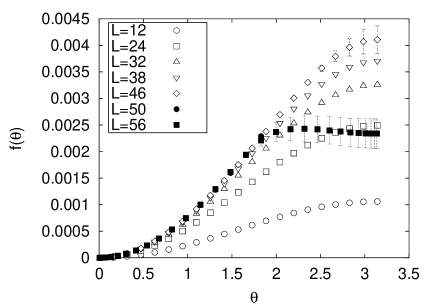
Figure 1: Free energy density $f(\theta)$ obtained from the MC data of the CP³ model. The coupling $\beta$ is fixed to 3.0 and lattice sizes $L$ are changed from 12 to 56. The number of measurements reaches several millions for each case.

Figure 1 displays $f(\theta)$ obtained from MC data of the CP³ model with the fixed point action. The coupling $\beta$ is fixed to 3.0 and various lattice sizes $L$ are employed. The number of measurements is several millions for each case. Although $f(\theta)$ for $L\leq 38$ behaves smoothly in the whole $\theta$ region, $f(\theta)$ for $L=50$ and 56 cannot be properly calculated for $\theta\hskip 3.00003pt\raisebox{1.72218pt}{$>$}\raisebox{-3.01385pt}{$\sim$}\hskip 3.00003pt2.0$. In the $L=56$ case, $f(\theta)$ becomes flat for $\theta\hskip 3.00003pt\raisebox{1.72218pt}{$>$}\raisebox{-3.01385pt}{$\sim$}\hskip 3.00003pt2.0$. This is called flattening. In the $L=50$ case, $f(\theta)$ cannot be obtained for $\theta\hskip 3.00003pt\raisebox{1.72218pt}{$>$}\raisebox{-3.01385pt}{$\sim$}\hskip 3.00003pt2.0$ due to negative values of ${\cal Z}(\theta)$. We also call it flattening, because the error in $P(Q)$ causes this behavior in the same way as the $L=56$ case. Flattening is originated from the sign problem. This is understood in the following way.[4, 5] The MC data of $P(Q)$ consists of the true value of $P(Q)$, ${\tilde{P}}(Q)$, and its error, $\Delta P(Q)$. When the error in $P(Q)$ at $Q=0$ dominates, $f(\theta)$ is approximated by $f(\theta)\simeq-\frac{1}{V}\log[e^{-V{\tilde{f}}(\theta)}+\Delta P(0)]$. Here, ${\tilde{f}}(\theta)$ denotes the true value of $f(\theta)$. Since $f(\theta)$ is an increasing function of $\theta$, $e^{V{\tilde{f}}(\theta)}\simeq|\Delta P(0)|$ could occur at $\theta=\theta_{\rm f}$ and $f(\theta)\simeq-\frac{1}{V}\log\delta P(0)$ for $\theta\hskip 3.00003pt\raisebox{1.72218pt}{$>$}\raisebox{-3.01385pt}{$\sim$}\hskip 3.00003pt\theta_{\rm f}$. To overcome this problem requires the number of measurements proportional to $e^{V}$.

3 MEM

The MEM is one of the parameter inference based on Bayes’ theorem and derives a unique solution by utilizing data and our knowledge about the parameters.[2, 3, 6] In our MEM analysis,[7, 8] the inverse Fourier transform

$$P(Q)=\int^{\pi}_{-\pi}d\theta\frac{e^{-i\theta Q}}{2\pi}{\cal Z}(\theta).$$ (2)

is used. The MEM involves to maximize the posterior probability ${\rm prob}({\cal Z}(\theta)|P(Q),I)$. Here,
${\rm prob}({\cal Z}(\theta)|P(Q),I)$ is the probability that ${\cal Z}(\theta)$ is realized when the MC data of $\{P(Q)\}$ and information $I$ are given. Information $I$ represents our state of knowledge about ${\cal Z}(\theta)$ and ${\cal Z}(\theta)>0$ is imposed. The probability is given by

$${\rm prob}({\cal Z}(\theta)|P(Q),I)\propto\exp\left[-\frac{1}{2}\chi^{2}+\alpha S\right]\equiv e^{W[{\cal Z}]},$$ (3)

where $\chi^{2}$, $\alpha$ and $S$ denote a standard $\chi^{2}$-function, a real positive parameter and an entropy, respectively. Conventionally, the Shannon-Jaynes entropy

$$S=\int_{-\pi}^{\pi}d\theta\left[{\cal Z}(\theta)-m(\theta)-{\cal Z}(\theta)\log\frac{{\cal Z}(\theta)}{m(\theta)}\right]$$ (4)

is employed. A function $m(\theta)$ is called default model and is chosen so as to be consistent with $I$. The most probable image ${\hat{\cal Z}}(\theta)$ is obtained according to the following procedures. (1) To obtain the most probable image for a given $\alpha$, ${\cal Z}^{(\alpha)}(\theta)$, by maximizing $W[{\cal Z}]$. (2) To obtain the $\alpha$-independent most probable image ${\hat{\cal Z}}(\theta)$ by averaging ${\cal Z}^{(\alpha)}(\theta)$ over $\alpha$; ${\hat{\cal Z}}(\theta)=\int d\alpha~{}P(\alpha){\cal Z}^{(\alpha)}(\theta)$. The probability $P(\alpha)$ represents the posterior probability of $\alpha$. (3) To estimate the error in ${\hat{\cal Z}}(\theta)$ as the uncertainty of ${\hat{\cal Z}}(\theta)$. The probability $P(\alpha)$ is given by $P(\alpha)\propto g(\alpha)e^{W(\alpha)+\Lambda(\alpha)}$. Here, $W(\alpha)\equiv W[{\cal Z}^{(\alpha)}]$, and $\Lambda(\alpha)$ represents contributions of fluctuations of ${\cal Z}(\theta)$ around ${\cal Z}^{(\alpha)}(\theta)$. The function $g(\alpha)$ is the prior probability of $\alpha$. Conventionally, two types of $g(\alpha)$ are used: $g_{\rm Lap}(\alpha)={\rm const}$ (Laplace’s rule) and $g_{\rm Jef}(\alpha)=1/\alpha$ (Jeffrey’s rule). Information about $\alpha$ before obtaining data does not play the conclusive role in the derivation of ${\hat{\cal Z}}(\theta)$. In the present study, the $g(\alpha)$-dependence of ${\hat{\cal Z}}(\theta)$ is estimated by the following quantity:

$$\Delta(\theta)\equiv\frac{|{\hat{\cal Z}}_{\rm Lap}(\theta)-{\hat{\cal Z}}_{\rm Jef}(\theta)|}{{\hat{\cal Z}}_{\rm Lap}(\theta)},$$ (5)

where ${\hat{\cal Z}}_{\rm Lap}(\theta)$ and ${\hat{\cal Z}}_{\rm Jef}(\theta)$ are the most probable images for Laplace’s and Jeffrey’s rules, respectively.

4 Numerical Results

We apply the MEM to the MC data with flattening as well as without flattening. The latter is the data for $L=38$ (data A) and the former is those for $L=50$ (data B). Here, two types of $m(\theta)$ are used: (i) Gaussian function $m_{\rm G}(\theta)=\exp[-\gamma\frac{\log 10}{\pi}\theta^{2}]$, where a parameter $\gamma$ is changed over a wide range, and (ii) $m(\theta)={\hat{\cal Z}}(\theta)$ for smaller volumes. In case (ii), to analyze the data for $L=L_{0}$, ${\hat{\cal Z}}(\theta)$ obtained by the MEM for smaller volumes are utilized as $m(\theta)$. For $L_{0}=50$, ${\hat{\cal Z}}(\theta)$ for $L=24$, 32 and 38 are used as $m(\theta)$, which are denoted as $m_{L/L_{0}}(\theta)=m_{L/50}(\theta)$. In this report, all results of the MEM with Laplace’s rule are shown except for $\Delta(\theta)$. In the analysis, the Newton method with quadruple precision is used.

4.1 Non Flattening Case

Figure 2 displays ${\hat{\cal Z}}(\theta)$ for data A. The Gaussian defaults $m_{\rm G}(\theta)$ with $\gamma=0.6$ and 1.0 are used. The partition function ${\cal Z}_{\rm Four}(\theta)$ obtained by the FTM is also plotted. Both the results of the MEM have no $m(\theta)$-dependence and are in agreement with the result of the FTM. The error of ${\hat{\cal Z}}(\theta)$, $\delta{\hat{\cal Z}}(\theta)$, are calculated according to the procedure (3). These errors are too small to be visible in Fig. 2.

Figure 2: The most probable images in the non flattening case ($L=38$). The result of the FTM is also plotted ($\times$).

4.2 Flattening Case

Let us turn to data B. Unlike data A, much care is needed in the analysis.[7] In order to properly evaluate ${\hat{\cal Z}}(\theta)$ as the final image, we investigate (i) the statistical fluctuation of ${\hat{\cal Z}}(\theta)$, (ii) $g(\alpha)$-dependence of ${\hat{\cal Z}}(\theta)$ and (iii) the relative error of ${\hat{\cal Z}}(\theta)$. In (i), it is found that the statistical fluctuation of ${\hat{\cal Z}}(\theta)$ becomes smaller with increasing the number of measurements and that ${\hat{\cal Z}}(\theta)$ with 20.0M/set is obtained with sufficiently small fluctuations except for near $\theta=\pi$. In (ii), we systematically investigate the $g(\alpha)$-dependence of ${\hat{\cal Z}}(\theta)$ by calculating $\Delta(\theta)$. The left panel of Fig. 3 displays $\Delta(\theta)$ at $\theta=2.60$, as a representative. Here, the Gaussian defaults are used, where $\gamma$ is changed from 3.0 to 13.5. The value of $\Delta(\theta)$ is the smallest for $\gamma=5.0$ and becomes larger as the value of $\gamma$ deviates from 5.0. Similar results are obtained in the whole $\theta$ region. This seems to indicate that $m_{\rm G}(\theta)$ with $\gamma=5.0$ is the most suitable as $m(\theta)$ among the defaults which we have chosen. Keeping in mind that $\Delta(\theta)$ includes an uncertainty originated from $\delta{\hat{\cal Z}}(\theta)$, we impose a constraint that the final images should satisfy $\Delta(\theta)<0.2$. Here, this value is chosen as a typical one of the uncertainty in $\Delta(\theta)$ coming from $\delta{\hat{\cal Z}}(\theta)$. Six images satisfy this constraint among those which we have obtained, and do not depend on $m(\theta)$ up to $\theta=3.0$. In (iii), we investigate how the MEM is applicable to our issue by calculating the relative error $|\delta{\hat{\cal Z}}(\theta)|/{\hat{\cal Z}}(\theta)$. Upon a constraint $|\delta{\hat{\cal Z}}(\theta)|/{\hat{\cal Z}}(\theta)<0.3$, the four most probable images ${\hat{\cal Z}}(\theta)$ satisfy the constraint up to $\theta=3.0$. This constraint is chosen from the fact that the error propagation of $P(Q)$ starts to strongly affect the behavior of ${\cal Z}_{\rm Four}(\theta)$ at $|\delta{\cal Z}_{\rm Four}(\theta)|/{\cal Z}_{\rm Four}(\theta)\simeq 0.3$ in the FTM (see the right panel of Fig. 4). Here, this value realizes at smaller value of $\theta$, $\theta=2.4$. These results are displayed in the right panel of Fig. 3.

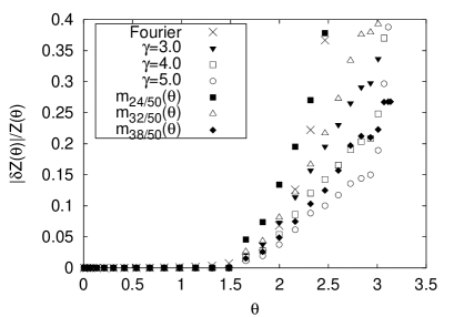
Figure 3: Values of $\Delta(\theta)$ at $\theta=2.60$ (left panel). The Gaussian defaults are used. Values of $|\delta{\hat{\cal Z}}(\theta)|/{\hat{\cal Z}}(\theta)$ for the selected 6 default models (right panel). The value of $|\delta{\cal Z}_{\rm Four}(\theta)|/{\cal Z}_{\rm Four}(\theta)$ is also plotted in the right panel.

In this analysis, we find that the four most probable images are obtained with reasonably small errors in a wide range of $\theta$, which is displayed in the left panel of Fig. 4. As a comparison, ${\cal Z}_{\rm Four}(\theta)$ is also shown in the right panel.

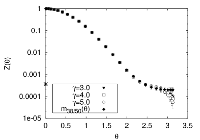
Figure 4: The most probable images for the selected $m(\theta)$ (left panel). As a comparison, ${\cal Z}_{\rm Four}(\theta)$ obtained by the FTM is also displayed in the right panel. The total number of measurements is 30.0M/set for both the cases.

5 Summary and Discussions

In this report, to deal with the sign problem in LFT with the $\theta$ term, we apply the MEM to the MC data of the CP³ model. In non flattening case, all results of the MEM agree with the one of the FTM within the errors. In the flattening case, obtained images depend on $m(\theta)$. By investigating whether they are adequate images, we have found that the MEM allows us to calculate ${\cal Z}(\theta)$ with small errors for large $\theta$ region. For the details, see Ref. [9]
Finally, let us make a brief comment about lattice QCD with the finite density in terms of the MEM. In lattice QCD with the finite chemical potential, MC simulation cannot be directly performed due to the complex phase of the fermion determinant. There are various techniques to avoid the sign problem and we concentrate on the canonical ensemble approach.[10, 11, 12, 13] By the fugacity expansion, ${\cal Z}(V,T,\mu)$ is written as

$${\cal Z}(V,T,\mu)=\sum_{n}Z(V,T,n)(e^{\mu/T})^{n},$$ (6)

where $n$ is the total quark number. Taking $\mu=i\phi T$, where $\phi$ is a real, ${\cal Z}(V,T,\mu=i\phi T)$ is free from the sign problem and ${\cal Z}(V,T,\mu=i\phi T)$, in principle, can be calculated with MC simulation. In this case, ${\cal Z}(V,T,\mu=i\mu T)=\sum_{n}Z(V,T,n)e^{in\phi}$. Comparing it with Eq. (2), we see the following correspondence:

$$\{P(Q)\leftrightarrow{\cal Z}(V,T,\mu=i\phi T),~{}e^{-i\theta Q}/2\pi\leftrightarrow e^{i\phi n},~{}{\cal Z}(\theta)\leftrightarrow Z(V,T,n)\}.$$ (7)

It may be worthwhile to study the theory in terms of the MEM.

References

- [1] C. Schmidt, hep-lat/0408047 and references in this paper.
- [2] R. K. Bryan, Eur. Biophys. J. 18 (1990), 165.
- [3] M. Jarrell and J. E. Gubarnatis, Phys. Rep. 269 (1996), 133.
- [4] J. C. Plefka and S. Samuel, Phys. Rev. D56 (1997), 44.
- [5] M. Imachi, S. Kanou and H. Yoneyama, Prog. Theor. Phys. 102 (1999), 653.
- [6] M. Asakawa, T. Hatsuda and Y. Nakahara, Prog. Part. Nucl. Phys. 46 (2001), 459.
- [7] M. Imachi, Y. Shinno and H. Yoneyama, Prog. Theor. Phys. 111 (2004), 387.
- [8] M. Imachi, Y. Shinno and H. Yoneyama, hep-lat/0506032
- [9] M. Imachi, Y. Shinno and H. Yoneyama, in progress.
- [10] A. Roberge and N. Weise, Nucl. Phys. B 275 (1986), 734.
- [11] A. Hasenfratz and D. Toussaint, Nucl. Phys. B 371 (1992), 539.
- [12] M. Alford, A. Kapustin and F. Wilzek, Phys. Rev. D 59 (1999), 05402.
- [13] A. Alexandru, N. Faber, I. Horváth and K.-F. Liu, hep-lat/0507020.