HU–EP–06/02
January 2006

Cooling, smearing and Dirac eigenmodes -
A comparison of filtering methods in lattice gauge theory

Starting from thermalized quenched SU(2) configurations we apply cooling or iterated smearing, respectively, to produce sequences of gauge configurations with less and less fluctuations. We compute the low lying spectrum and eigenmodes of the lattice Dirac operator and compare them for the two types of smoothing. Many characteristic properties of the eigensystem remain invariant for all configurations in our sequences. We also find that cooling and smearing produce surprisingly similar results. Both observations could be indications that the two filtering methods do not drastically alter the long range structures in the gauge field.

1 Introduction

An appealing feature of numerical lattice QCD is that it allows for a direct access to gluon field configurations as they appear in the fully quantized path integral. The motivation for their analysis is the hope to identify the key mechanisms giving rise to the characteristic features of confinement and chiral symmetry breaking. Unfortunately, a naive look at, e.g., the action density reveals only quantum fluctuations. However, it is widely believed that underneath these UV fluctuations long range structures are hidden which might be stabilized by topology.

When analyzing these infrared structures a filter for removing the quantum fluctuations is necessary. Three main approaches can be found in the literature. Cooling is essentially a Monte Carlo update which accepts only changes that lower the action, thus finally driving the configuration into a classical solution. Smearing is an operation which combines neighboring gauge variables to average out short distance fluctuations. Repeated application thus also gives rise to smoother and smoother gluon configurations. Both, cooling and smearing do actually change the gauge field to extract its IR content. Thus an obvious criticism of these two approaches is the uncertainty whether the filtering does not also destroy or at least considerably change the long range structures one is interested in.

An alternative which has become widely popular in the last few years $\!{}^{{\bf?}}$ is the analysis of low lying eigenmodes of the lattice Dirac operator and very recently also of the covariant Laplace operator $\!{}^{{\bf?}}$. It is expected that the low lying eigenmodes couple mainly to the infrared structures of the gauge field. Obviously the method leaves the gauge field untouched while exploring the long range structures. It is considered to be a particularly “physical” filter since the IR content of the gluon field is “seen through the eyes of the quarks”.

However, a big disadvantage of eigenmode filtering is that purely gluonic quantities such as the field strength, the action- and charge densities, or the Polyakov loop have to be reconstructed in a non-trivial way $\!{}^{{\bf?},{\bf?}}$, or are not accessible at all. Since these gluonic observables provide important information for many physical questions, it is desirable to have an alternative to the fermionic filter, which at the same time guarantees that the long range structures are not altered.

In this little study we address in a new way the question whether cooling $\!{}^{{\bf?},{\bf?}}$ or smearing $\!{}^{{\bf?}}$ alter the infrared content of the gauge field: We use observables based on the low lying Dirac eigenmodes and analyze how they change under cooling or repeated smearing. If such fermionic observables change considerably in a sequence of smoother and smoother configurations, this is a strong indication that the IR structures are altered by the smoothing method applied. Here we present evidence that for many steps of smoothing (cooling or smearing) the fermionic observables remain essentially invariant. Furthermore we find that the two smoothing methods we use, cooling and smearing, lead to very similar results.

2 Technicalities

Our study is based on quenched SU(2) configurations generated with the Lüscher-Weisz gauge action $\!{}^{{\bf?}}$ at $\beta=1.95$ on lattices of size $16^{4}$. We use periodic boundary conditions for the gauge fields. As outlined in the introduction, we generate from the original, thermalized configurations sequences of smoother and smoother configurations by applying either cooling or smearing.

In our cooling procedure we run the same single link Metropolis update used for generating the thermalized configurations but omit the conditional acceptance step for the case where the offered gauge configuration leads to an increased action. The offer is chosen relatively close to the old link variable (see also restricted cooling $\!{}^{{\bf?}}$). This implies that our cooling is very modest and we can produce sequences of cooled configurations with only small changes in each sweep. The number of cooling sweeps was chosen such that the average plaquette matches the value obtained by smearing (compare Table 1).

The 4-dimensional smearing of our Monte Carlo gauge field configurations has been performed in the standard way of sequential substitution sweeps:

$$U^{(j)}_{x,\mu}\to U^{(j+1)}_{x,\mu} = \mathrm{Proj}_{SU(2)}\bigg{[}\;\alpha\,U^{(j)}_{x,\mu}$$

$$+ \gamma\sum_{\nu\neq\mu}\left(U^{(j)}_{x,\nu}U^{(j)}_{x+\hat{\nu},\mu}U^{(j)\dagger}_{x+\hat{\mu},\nu}+U^{(j)\dagger}_{x-\hat{\nu},\nu}U^{(j)}_{x-\hat{\nu},\mu}U^{(j)}_{x-\hat{\nu}+\hat{\mu},\nu}\right)\bigg{]}\;,$$

with $\alpha=0.55$ and $\gamma=(1-\alpha)/6=0.075$. Obviously, this standard smearing is not adapted to any specific action that has been used for the generation of the Monte Carlo ensemble.

cooling		smearing
sweeps	$\langle U_{p}\rangle$	sweeps	$\langle U_{p}\rangle$
0	0.695165	0	0.695165
8	0.884064	1	0.885551
19	0.948482	2	0.949688
38	0.973993	3	0.974081
72	0.984799	4	0.984740
140	0.990499	5	0.990010
220	0.992822	6	0.992907
360	0.994559	7	0.994647
580	0.995730	8	0.995771
900	0.996520	9	0.996541
1360	0.997089	10	0.997093

Table 1: Comparison of key numbers for a cooling and a smearing sequence, both starting from the same thermalized configuration. We display the number of cooling- and smearing steps respectively and the corresponding value of the average plaquette. The number of cooling sweeps was chosen such that the cooled configuration matches the action of the corresponding smeared configuration as close as possible. ${}^{\;}$

We consider a total of 10 thermalized configurations and apply to each of them 10 sweeps of smearing, storing the configurations after each sweep. Starting from the same 10 thermalized configurations we also apply suitable numbers of cooling sweeps such that the action is as close as possible to the corresponding smeared configurations. Thus we end up with two times 10 sequences of configurations each consisting of the original gauge field and 10 increasingly smoothed configurations. For these sequences of cooled, respectively smeared configurations we calculate the lowest 30 eigenvalues and eigenvectors of the lattice Dirac operator with the Arnoldi method $\!{}^{{\bf?}}$. We use the chirally improved Dirac operator $\!{}^{{\bf?}}$, an approximate solution of the Ginsparg-Wilson equation $\!{}^{{\bf?}}$, which is the optimal implementation of chiral symmetry on the lattice.

Of the 10 thermalized configurations we analyze, 2 have topological charge $Q=0$, 6 have $|Q|=1$ and the remaining 2 are in the sector $|Q|=2$, with the topological charge determined via the index theorem through the number of left- or right-handed zero modes.

We compute the eigensystem for both, periodic and anti-periodic temporal boundary conditions, leaving the spatial boundary conditions periodic. The motivation for two different temporal boundary conditions is that for finite temperature it is known $\!{}^{{\bf?}}$ that the zero modes are localized on monopole-like constituents of so-called Kraan-van Baal calorons $\!{}^{{\bf?}}$ which may be located at different space-time positions. Also for configurations on the torus the corresponding hopping of the zero modes has been observed for gauge group SU(2) and SU(3) $\!{}^{{\bf?}}$. Here we want to probe the sequences of configurations with the eigensystem of the Dirac operator, and the hopping of the zero modes under a change of boundary conditions is highly welcome as an additional signature.

The base quantity for our fermionic observables is the scalar density

$$\rho(x)\;=\;\sum_{c,\alpha}|v_{c,\alpha}(x)|^{2}\;,$$ (2)

obtained by locally summing the absolute square for each entry of a Dirac eigenvector $v$ over its color and Dirac indices $c$ and $\alpha$. In order to determine the location of a mode we use the maximum of $\rho(x)$. Using 3-d plots of $\rho(x)$ over slices of the lattice (see Fig. 2) we can further analyze the eigenmodes. A quantity which condenses the localization properties of eigenmodes into a single number is the inverse participation ratio

$$IPR\;=\;V\sum_{x}\rho(x)^{2}\;.$$ (3)

Using the fact that $\sum_{x}\rho(x)=1$ (our eigenvectors are normalized to 1), it is easy to see that the inverse participation ratio reaches its maximum value $IPR=V$ for a density $\rho$ which is 1 for a single site and 0 everywhere else, while for a completely spread out eigenmode ($\rho(x)\equiv 1/V$) one finds $IPR=1$.

3 Results

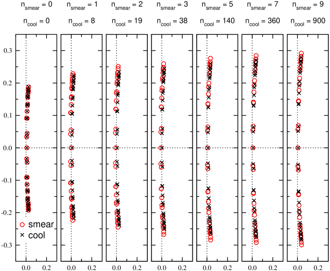
Figure 1: Spectra of the Dirac operator in the complex plane. The circles represent eigenvalues for the sequence of configurations obtained by smearing, the crosses are used for the cooled configurations. In each spectrum the 30 smallest eigenvalues for periodic boundary conditions are shown. ${}^{\;}$

3.1 Eigenvalues and topological charge

We begin the presentation of our results with the discussion of the eigenvalues and their change under the two smoothing procedures. Fig. 1 shows the 30 lowest lying eigenvalues of the Dirac operator in the complex plane for one pair of our sequences. The circles are used for the smeared configurations, while the crosses represent the results for cooling. The left-most spectrum is for the original, thermalized configuration and as one moves to the right the amount of smoothing increases. The corresponding numbers of cooling and smearing steps respectively are denoted at the top of each individual plot.

A feature, which is obvious from the plots, is that when smoothing the configurations, the spectrum becomes less dense and the eigenvalue density is reduced. Smearing stretches the spectrum slightly stronger, thus reducing the eigenvalue density by a few percent more than cooling. Otherwise the eigenvalues, in particular the lowest lying ones, behave almost identically under cooling and smearing, and the symbols lie nearly on top of each other. Also for the higher lying eigenvalues the characteristic patterns for their grouping are kept by both smoothing methods.

The configuration we have used for Fig. 1 has a single, left-handed zero mode and through the index theorem thus can be seen to have topological charge $Q=1$. The existence of this zero mode is not altered by the two smoothing procedures. This observation holds for all our 10 pairs of sequences: The topological charge as determined by the index theorem did never change under the cooling or smearing we applied. We should however remark that much longer sequences of cooling or smearing will certainly destroy the topological charge and thus lead to a vanishing of the corresponding zero mode.

We remark that for staggered fermions it was shown $\!{}^{{\bf?}}$ in a similar way that under smearing the spectral properties become more transparent then. A version of the index theorem, suitable for staggered fermions, can be established.

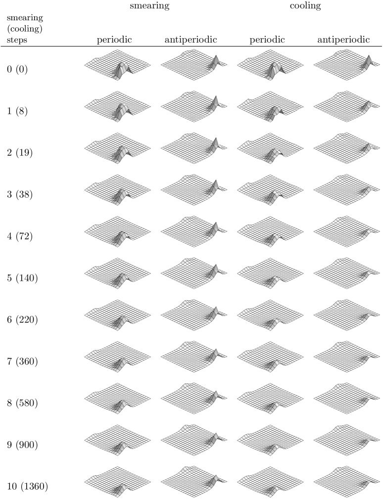
Figure 2: Scalar density of a zero mode for periodic and anti-periodic boundary conditions. The two columns on the left-hand side are for the sequence of configurations generated with smearing, while the two columns on the right-hand side are for the corresponding sequence from cooling. For both, periodic and anti-periodic boundary conditions we show the $xy$-slice through the respective maximum. ${}^{\;}$

3.2 Scalar density and the role of the boundary condition

Let us now address the behavior of the eigenmodes under smoothing. In particular we here focus on the 6 configurations with exactly one eigenvalue zero and present results for the corresponding zero modes. As announced, our basic observable is the scalar density $\rho(x)$, and in a first step we look for the lattice site where it assumes a maximum. Subsequently we study the scalar density over slices of the lattice cut through the maximum. For our 4-dimensional lattice we have 6 different slices and we typically find that the lumps in the scalar density are localized in all 4 directions. Thus defining the location of an infrared lump through the position of its maximum is a meaningful procedure.

In Fig. 2 we show 3-d plots of $\rho(x)$ over one of the slices and follow the evolution of the lump as we apply more and more filtering (top to bottom). The two columns on the left-hand side are for smearing, while the two right-hand side columns are for the corresponding cooled sequence. It is obvious from the plots that the position of the lump remains unchanged as the configurations become smoother and smoother. For both methods the height of the lumps decreases for the smoother configurations, but their width is not altered drastically. Cooling seems to have the tendency to remove spiky structures faster than smearing, which is on the other hand obvious since such spikes cost a lot of action which is systematically reduced by cooling.

For some of our configurations we find that the position of the lump in the zero mode changes when switching the temporal boundary condition from periodic to anti-periodic. Often the mode is then located at a completely different site of the lattice and the spot where $\rho(x)$ showed a peak before now has a flat distribution of $\rho(x)$. Thus for some of our $|Q|=1$ configurations we find two “hot spots” where the lump in the zero mode density is located. In Fig. 2 we use a configuration which shows hopping and show the slices through the respective maxima for both boundary conditions as indicated in the header for each column. We find that both, cooling and smearing, detect the same hot spots and thus also in this respect behave essentially identical.

We found that for some configurations the hopping can stop after a certain amount of smoothening and the zero mode settles at a single position. Also for such cases we established that cooling and smearing behave essentially identically, and for 5 of our 6 $|Q|=1$ configurations we found that the pattern for the hot spots agrees between the cooled sequence and its smeared counterpart.

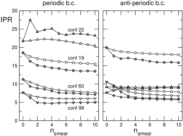
Figure 3: The inverse participation ratio of zero modes as a function of the number of smearing (cooling) steps. The open symbols are for smearing, while the filled symbols represent the results from configurations with an equivalent number of cooling steps (compare Table 1). The left-hand side plot is for periodic boundary conditions, the right-hand side plot for the anti-periodic case. ${}^{\;}$

Let us finally come to the comparison of the behavior of the inverse participation ratio $IPR$ under our two smoothing methods. In Fig. 3 we show the history of IPR under cooling (filled symbols) and smearing (open symbols). On the horizontal axis for simplicity we only display the number of smearing steps. The number of cooling steps, giving rise to configurations with equivalent action, is as listed in Table 1. The left-hand side plot is for periodic temporal boundary conditions, the right-hand side is for the anti-periodic case.

For all cases cooling and smearing give rise to similar histories for the inverse participation ratio. The values of $IPR$ remain in the same range, although cooling typically produces somewhat smaller numbers (except for one case). This is in agreement with the above observation, that cooling tends to cut spiky structures with their generically higher inverse participation ratio.

4 Summary and conclusions

In this contribution we present a comparison of smearing and cooling for the removal of short range ultraviolet fluctuations from quenched SU(2) configurations. The observables we use for this comparison are entirely based on the eigensystem of the Dirac operator. The low lying Dirac eigenmodes couple to the long range structures of the gluon field and allow to study them without any manipulation of the gauge configuration. Thus the fermionic observables are very suitable tools for comparing the different methods of smoothing.

We find that the two methods we apply, cooling and smearing, lead to surprisingly similar results: Patterns in the eigenvalue spectrum, characteristic for individual configurations are conserved to a large degree by both smoothing methods. Furthermore, the topological charge as determined by the index theorem remains unchanged in the range of smoothing we consider. When analyzing the eigenvectors, we find that the shapes of lumps in the scalar density change in the same way for cooling and smearing: The lumps essentially only decrease in height, but remain at their position. Also the hopping patterns of the zero modes under a change of the boundary conditions are essentially the same when applying cooling or smearing. A similar observation holds for the inverse participation ratio which expresses the localization properties of eigenmodes as a single number.

How should our findings be interpreted? We have motivated this study by the quest for the perfect filter for long range structures in lattice gauge configurations. Our results seem to indicate that, at least for fermionic observables, the two filtering methods applied, cooling and smearing, lead to a relatively similar outcome. This could imply that the smoothing methods are maybe less arbitrary than they seem at first glance and indeed leave the long range structures of the original configuration relatively unchanged, at least for the amount of smoothing considered here. Certainly, this interpretation needs to be further tested by analyzing more fermionic observables, as well as different gauge actions and the gauge group SU(3). Also the evaluation of gluonic observables on the sequences of configurations should be attempted. Both these issues will be addressed in an upcoming study.

References

References

- [1] T.L. Ivanenko and J.W. Negele, Nucl. Phys. Proc. Suppl. 63 (1998) 504; J.W. Negele, Nucl. Phys. A 670 (2000) 14; C. Gattringer and I. Hip, Nucl. Phys. B 536 (1998) 363, Nucl. Phys. B 541 (1999) 305, Nucl. Phys. Proc. Suppl. 73 (1999) 871; I. Horváth, N. Isgur, J. McCune, and H.B. Thacker, Phys. Rev. D 65 (2002) 014502; T. De Grand and A. Hasenfratz, Phys. Rev. D 65 (2002) 014503; I. Hip, Th. Lippert, H. Neff, K. Schilling, and W. Schroers, Phys. Rev. D 65 (2002) 014506; R.G. Edwards and U.M. Heller, Phys. Rev. D 65 (2002) 014505; T. Blum et al., Phys. Rev. D 65 (2002) 014504; C. Gattringer et al., Nucl. Phys. B 617 (2001) 101, Nucl. Phys. B 618 (2001) 205, Nucl. Phys. Proc. Suppl. 106 (2002) 551; I. Horvath et al., Phys. Rev. D 66 (2002) 034501, Phys. Rev. D 67 (2003) 011501, Phys. Rev. D 68 (2003) 114505, Nucl. Phys. B 710 (2005) 464 [Erratum-ibid. B 714 (2005) 175], Phys. Lett. B 612 (2005) 21 [arXiv:hep-lat/0501025]; C. Aubin et al. [MILC Collaboration], Nucl. Phys. Proc. Suppl. 140 (2005) 626; C. Bernard et al., PoS LAT2005 (2005) 299; J. Gattnar et al., Nucl. Phys. B 716 (2005) 105, PoS LAT2005 (2005) 301; F.V. Gubarev, S.M. Morozov, M.I. Polikarpov, and V.I. Zakharov, JETP Lett. 82 (2005) 343. V. Kovalenko, S.M. Morozov, M.I. Polikarpov, and V.I. Zakharov, arXiv:hep-lat/0512036; M.N. Chernodub and S.M. Morozov, arXiv:hep-lat/0512041.
- [2] J. Greensite, S. Olejnik, M. Polikarpov, S. Syritsyn, and V.I. Zakharov Phys. Rev. D71 (2005) 114507; F. Bruckmann and E.-M. Ilgenfritz, Phys. Rev. D 72 (2005) 114502; F. Bruckmann and E.-M. Ilgenfritz, PoS LAT2005 (2005) 305; F. Bruckmann and E.-M. Ilgenfritz, arXiv:hep-lat/0511030.
- [3] C. Gattringer, Phys. Rev. Lett. 88 (2002) 221601.
- [4] E.-M. Ilgenfritz, M.L. Laursen, G. Schierholz, M. Müller-Preussker, and H. Schiller, Nucl. Phys. B268 (1986) 693.
- [5] M. Campostrini, A. Di Giacomo, and H. Panagopoulos, Nucl. Phys. B329 (1990) 683; M. Campostrini, A. Di Giacomo, M. Maggiore, H. Panagopoulos, and E. Vicari, Phys. Lett. B225 (1989) 403.
- [6] T. DeGrand, A. Hasenfratz, and T.G. Kovacs, Nucl. Phys. B 520 (1998) 301.
- [7] M. Lüscher and P. Weisz, Commun. Math. Phys. 97 (1985) 59, Err.: 98 (1985) 433; G. Curci, P. Menotti, and G. Paffuti, Phys. Lett. B 130 (1983) 205, Err.: B 135 (1984) 516.
- [8] D.C. Sorensen, SIAM J. Matrix Anal. Appl. 13 (1992) 357; R.B. Lehoucq, D.C. Sorensen, and C. Yang, ARPACK User’s Guide, SIAM, New York, 1998.
- [9] C. Gattringer, Phys. Rev. D 63 (2001) 114501; C. Gattringer, I. Hip, and C.B. Lang, Nucl. Phys. B597 (2001) 451.
- [10] P.H. Ginsparg and K.G. Wilson, Phys. Rev. D 25 (1982) 2649.
- [11] E.-M. Ilgenfritz, B.V. Martemyanov, M. Müller-Preussker, S. Shcheredin, and A.I. Veselov, Phys. Rev. D 66 (2002) 074503; M. Garcia Pérez, A. González-Arroyo, C. Pena, and P. van Baal, Phys. Rev. D 60 (1999) 031901; M.N. Chernodub, T.C. Kraan, and P. van Baal, Nucl. Phys. Proc. Suppl. 83 (2000) 556; C. Gattringer et al., Nucl. Phys. Proc. Suppl. 129 (2004) 653; C. Gattringer and S. Schaefer, Nucl. Phys. B 654 (2003) 30; C. Gattringer, Phys. Rev. D 67 (2003) 034507; F. Bruckmann, D. Nogradi, and P. van Baal, Nucl.Phys. B666 (2003) 197.
- [12] T.C. Kraan and P. van Baal, Phys. Lett. B 428 (1998) 268, ibid. B 435 (1998) 389, Nucl. Phys. B 533 (1998) 627; K. Lee and C. Lu, Phys. Rev. D 58 (1998) 1025011.
- [13] C. Gattringer and S. Solbrig, arXiv:hep-lat/0410040; C. Gattringer and R. Pullirsch, Phys. Rev. D 69 (2004) 094510.
- [14] S. Dürr, C. Hoelbling, and U. Wenger, Phys. Rev. D 70 (2004) 094502; Nucl. Phys. Proc. Suppl. 140 (2005) 677.