Lattice Flavourdynamics 

Abstract

I present a selection of recent lattice results in flavourdynamics, including the status of the calculation of quark masses and a variety of weak matrix elements relevant for the determination of CKM matrix elements. Recent improvements in the momentum resolution of lattice computations and progress towards precise computations of $K\to\pi\pi$ decay amplitudes are also reviewed.

1 Introduction

One of the main approaches to testing the Standard Model of Particle Physics and searching for signatures of new physics is to study a large number of physical processes to obtain information about the unitarity triangle and to check its consistency. The precision with which this check can be accomplished is limited by non-perturbative QCD effects and lattice QCD provides the opportunity to quantify these effects without model assumptions. Of course, lattice computations themselves have a number of sources of systematic uncertainty, and much of our current effort is being devoted to reducing and controlling these errors. In this talk I briefly discuss the evaluation of quark masses and weak matrix elements using lattice simulations.

For most lattice calculations of physical quantities, the principal source of systematic uncertainty is the chiral extrapolation, i.e. the extrapolation of results obtained with unphysically large $u$ and $d$ quark masses. Ideally we would like to perform computations with 140 MeV pions and hence with $m_{q}/m_{s}$ of about 1/25 (where $m_{q}$ ($m_{s}$) is the average light quark mass (strange quark mass)). In practice values $m_{q}/m_{s}\geq$ 1/2 are fairly typical, so that the MILC Collaboration’s simulation with $m_{q}/m_{s}\simeq 1/8$ is particularly impressive bernard and provides a challenge to the rest of the community to reach similarly low masses. Its configurations have been widely used to determine physical quantities with small quoted errors.

The MILC collaboration uses the staggered formulation of lattice fermions and for a variety of reasons it is very important to verify the results using other formulations. With staggered fermions each meson comes in 16 tastes and the unphysical ones are removed by taking the fourth root of the fermion determinant. Although there is no demonstration that this procedure is wrong, there is also no proof that it correctly yields QCD in the continuum limit durr . The presence of unphysical tastes leads to many parameters to be fit in staggered chiral perturbation theory (typically many tens of parameters) and to date the renormalization has only been performed using perturbation theory. It is therefore pleasing to observe that the challenge of reaching lower masses is being taken up by groups using other formulations of lattice fermions (see e.g. ref. luscherdublin ) .

In this talk I will discuss a selection of issues and results in lattice flavourdynamics. I start by describing some new thoughts on improving the momentum resolution in simulations, by varying the boundary conditions on the quark fields. I then review the status of lattice calculations of quark masses, $K_{\ell 3}$ decays (for which computations have only recently began) and $B_{K}$. This is followed by a discussion of some of the key issues in the computation of $K\to\pi\pi$ decays and in heavy-quark physics.

1.1 Improving the Momentum Resolution on the Lattice

Numerical simulations of lattice QCD are necessarily performed on a finite spatial volume, $V=L^{3}$. Providing that $V$ is sufficiently large, we are free to choose any consistent boundary conditions for the fields $\phi(\vec{x},t)$, and it is conventional to use periodic boundary conditions, $\phi(x_{i}+L)=\phi(x_{i})$ ($i=1,2$ or 3). This implies that components of momenta are quantized to take integer values of $2\pi/L$. Taking a typical example of a lattice with 24 points in each spatial direction, $L=24a$, with a lattice spacing $a=0.1$ fm so that $a^{-1}\simeq 2$ GeV, we have $2\pi/L=.52$ GeV. The available momenta for phenomenological studies (e.g. in the evaluation of form-factors) are therefore very limited, with the allowed values of each component $p_{i}$ separated by about 1/2 GeV. The momentum resolution in such simulations is very poor.

Bedaque bedaque has advocated the use of twisted boundary conditions for the quark fields $q(\vec{x})$ e.g.

$$q(x_{i}+L)=e^{i\theta_{i}}q(x_{i})\quad\textrm{with momentum spectrum}\quad p_{i}=n_{i}\frac{2\pi}{L}+\frac{\theta_{i}}{L}\,,$$ (1)

with integer $n_{i}$. Modifying the boundary conditions changes the finite-volume effects, however, for quantities which do not involve Final State Interactions (e.g. hadronic masses, decay constants, form-factors) these errors remain exponentially small also with twisted boundary conditions giovanni . Since we usually neglect such errors when using periodic boundary conditions, we can use twisted boundary conditions with the same precision. Moreover the finite-volume errors are also exponentially small for partially twisted boundary conditions in which the sea quarks satisfy periodic boundary conditions but the valence quarks satisfy twisted boundary conditions giovanni ; chen . This is of significant practical importance, implying that we do not need to generate new gluon configurations for every choice of twisting angle $\{\theta_{i}$}.

The use of partially twisted boundary conditions opens up many interesting phenomenological applications, solving the problem of poor momentum resolution. It also appears to work numerically. Consider for example, the plots in fig. 1, obtained using an unquenched (2 flavours of sea quarks) UKQCD simulation on a $16^{3}\times 32$ lattice, with a spacing of about 0.1 fm. The plots correspond to a value for the light-quark masses for which $m_{\pi}/m_{\rho}=0.7$  juettner . The lower (upper) left-hand plot shows the energy of the $\pi$ ($\rho$) as a function of the momentum of the meson, and the right-hand plot shows the bare values of the leptonic decay constants $f_{\pi}$ and $f_{\rho}$. The $x$-axis denotes $(|\vec{p}\,|L)^{2}$. The results are beautifully consistent with expectations (particularly for $pL\leq 2\pi$ where lattice artifacts are small); the predicted dispersion relation is satisfied and the extracted decay constants are independent of the momenta. Using periodic boundary conditions only the results at values of $\vec{p}$ indicated by the dashed lines are accessible. With partially twisted boundary conditions all momenta are reachable.

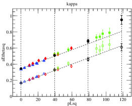
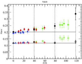
Figure 1: Plots of the Dispersion Relation (left) and Decay Constants (right) as a function of the momentum $\vec{p}$ of the mesons. In both cases the top (bottom) plot corresponds to the $\rho$-meson ($\pi$-meson).

2 Quark Masses

Quark Masses are fundamental parameters of the Standard Model, but unlike leptons, quarks are confined inside hadrons and are not observed as physical particles. Quark masses therefore cannot be measured directly, but have to be obtained indirectly through their influence on hadronic quantities and this frequently involves non-perturbative QCD effects. Lattice simulations prove to be very useful in the determination of quark masses; particularly for the light quarks ($u,d$ and $s$) for which perturbation theory is inapplicable.

In order to determine the quark masses we compute a convenient and appropriate set of physical quantities (frequently a set of hadronic masses) and vary the input masses until the computed values correctly reproduce the set of physical quantities being used for calibration. In this way we obtain the physical values of the bare quark masses, from which by using perturbation theory, or preferably non-perturbative renormalization, the results in standard continuum renormalization schemes can be determined.

My current best estimates for the values of the quark masses as determined from lattice simulations are presented in table 1.

Flavour	Best Lattice Values	PDG 2004 (Lattice)	PDG 2004 (Non-Lattice)
$\hat{m}(2\,\textrm{GeV})$	($3.8\pm 0.8$) MeV	($4.2\pm 1.0$) MeV	$(1.5<m_{u}(2\,\textrm{GeV})<5)$ MeV
			$(5<m_{d}(2\,\textrm{GeV})<9)$ MeV
$m_{s}(2\,\textrm{GeV})$	$(95\pm 20)\,$MeV	$(105\pm 25)\,$MeV	80 – 155 MeV
$\bar{m}_{c}$	$(1.26\pm 0.13\pm 0.20)$ GeV	$(1.30\pm 0.03\pm 0.20)$ GeV	1 – 1.4 GeV
$\bar{m}_{b}$	$(4.2\pm 0.1\pm 0.1)$ GeV	$(4.26\pm 0.15\pm 0.15)$ GeV	4 – 4.5 GeV

Table 1: My summary of the status of lattice determinations of quark masses (in the $\overline{\textrm{MS}}$ renormalization scheme). For $\hat{m}\equiv(m_{u}+m_{d})/2$ and $m_{s}$ the results are presented at 2 GeV and for $m_{c},\,m_{b}$, the results are presented at the mass itself ($\bar{m}\equiv\bar{m}(\bar{m})$) . For comparison the values quoted by the PDG in 2004, using or excluding lattice simulations, are also presented.

The relatively large error on the mass of the charm quark is a reflection of the fact that the most detailed study to date was performed in the quenched approximation rolf , whose authors find $\bar{m}_{c}=1.301(34)\,\textrm{GeV}$. I have added a conservative 15% error as an estimate of quenching effects. Current and future calculations will be dominated by unquenched simulations so that the error will decrease very significantly. Indeed a very recent unquenched calculation finds $\bar{m}_{c}=1.22(9)$ GeV nobes .

The relative error on $m_{b}$ is small because what is actually calculated is $m_{B}-m_{b}$. The calculations are performed in the Heavy Quark Effective Theory and the major source of systematic error is the subtraction of $O(1/(a\Lambda_{\textrm{QCD}}))$ terms. Using stochastic perturbation theory, Di Renzo and Scorzato have performed this calculation to 3-loop order direnzo . The second error on $\bar{m}_{b}$ in table 1 is my conservative estimate of the fact that the simulations have been performed with two flavours of sea quarks.

3 Selected Topics in Kaon Physics

3.1 $K_{\ell 3}$ Decays

A new area of investigation for lattice simulations is the evaluation of non-perturbative QCD effects in $K\to\pi\ell\nu_{\ell}$ decays, from which the CKM matrix element $V_{us}$ can be determined. The QCD contribution to the amplitude is contained in two invariant form-factors $f^{0}(q^{2})$ and $f^{+}(q^{2})$ defined by

$$\langle\,\pi(p_{\pi})\,|\bar{s}\gamma_{\mu}u\,|\,K(p_{K})\,\rangle=f^{0}(q^{2})\,\frac{M_{K}^{2}-M_{\pi}^{2}}{q^{2}}q_{\mu}+f^{+}(q^{2})\,\left[(p_{\pi}+p_{K})_{\mu}-\frac{M_{K}^{2}-M_{\pi}^{2}}{q^{2}}q_{\mu}\right]\,,$$

where $q=p_{K}-p_{\pi}$. (Parity Invariance implies that only the vector current from the $V-A$ charged current contributes to the decay.) A useful reference value for $f^{+}(0)$ comes from the 20-year old prediction of Leutwyler and Roos, $f^{+}(0)=1+f_{2}+f_{4}+\cdots=0.961(8)$ where $f_{n}=O(M^{2}_{K,\pi,\eta})$. $f_{2}=-0.023$ is well determined, whereas the higher order terms in the chiral expansion require model assumptions.

To be useful in extracting $V_{us}$ from experimental measurements we need to be able to evaluate $f^{0}(0)=f^{+}(0)$ to better than about 1% precision. This would seem to be impossible until one notes that it is possible to compute $1-f^{+}(0)$, so that an error of 1% on $f^{+}(0)$ is actually an error of O(25%) on $1-f^{+}(0)$. The calculation follows a similar strategy to that proposed in ref. hashimoto for the form-factors of $B\to D$ semileptonic decays (which in the heavy quark limit are also close to 1), starting with a computation of double ratios such as

$$\frac{\langle\pi|\bar{s}\gamma_{0}l|K\rangle\langle K|\bar{l}\gamma_{0}s|\pi\rangle}{\langle\pi|\bar{l}\gamma_{0}l|\pi\rangle\langle K|\bar{s}\gamma_{0}s|K\rangle}=\left[f^{0}(q^{2}_{\textrm{max}})\right]^{2}\,\frac{(m_{K}+m_{\pi})^{2}}{4m_{K}m_{\pi}}\,,$$ (2)

where all the mesons are at rest and $q^{2}_{\textrm{max}}=(M_{K}-M_{\pi})^{2}$.

Following a quenched calculation by the SPQR collaboration last year spqrkl3 , in which the strategy for determining the form-factors was presented, there have been 3 very recent unquenched (albeit largely preliminary) results:

RBC rbckl3	$f^{+}(0)$ = 0.955 (12)
JLQCD jlqcdkl3	$f^{+}(0)$ = 0.952 (6)
FNAL/MILC/HPQCD milckl3	$f^{+}(0)$ = 0.962 (6) (9)

in good agreement with the result of Leutwyler and Roos leutwyler .

3.2 $B_{K}$

$B_{K}$, the parameter which contains the non-perturbative QCD effects in $K^{0}-\bar{K}^{0}$ mixing, has been computed in lattice simulations by many groups. It is defined by

$$\langle\bar{K}^{0}\,|\,(\bar{s}\gamma^{\mu}(1-\gamma^{5})d)\,(\bar{s}\gamma_{\mu}(1-\gamma^{5})d)|K^{0}\rangle=\frac{8}{3}\,M_{K}^{2}\,f_{K}^{2}\,B_{K}\,.$$ (3)

$B_{K}$ depends on the renormalization scheme and scale and is conventionally given in the NDR, $\overline{\textrm{MS}}$ scheme at $\mu=2\,$GeV or as the RGI parameter $\hat{B}_{K}$ (the relation between the two is $\hat{B}_{K}\simeq 1.4\ B_{K}^{\overline{\textrm{MS}}}(2\,\textrm{GeV})$).

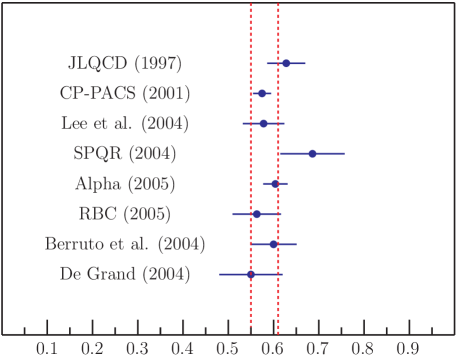
Figure 2: A compilation of recent quenched results for $B^{\overline{MS}}_{K}(2\,\textrm{GeV})$.

A compilation of recent results for $B_{K}$ obtained in the quenched approximation is presented in fig. 2. From such results recent reviewers have summarised the status of quenched calculations as:

$$B^{\overline{MS}}_{K}(2\,\textrm{GeV})=0.58(4)~{}\textrm{\cite[cite]{\@@bibref{Authors Phrase1YearPhrase2}{hashimotoichep}{\@@citephrase{(}}{\@@citephrase{)}}}}\quad\textrm{and}\quad B^{\overline{MS}}_{K}(2\,\textrm{GeV})=0.58(3)~{}\textrm{\cite[cite]{\@@bibref{Authors Phrase1YearPhrase2}{dawsondublin}{\@@citephrase{(}}{\@@citephrase{)}}}}\,.$$ (4)

The dashed lines in fig. 2 correspond to $B_{K}=.58(3)$, which I am happy to take as the current best estimate.

The challenge now is to obtain reliable unquenched results; such computations are underway by several groups but so far the results are very preliminary. We will have to wait a year or two for precise results, but I mention in passing C.Dawson’s guesstimate dawsondublin (stressing that it is only a guesstimate), based on a comparison of quenched and unquenched results at similar masses and lattice spacings, of $B^{\overline{MS}}_{K}(2\,\textrm{GeV})=0.58(3)(6)$.

3.3 $K\to\pi\pi$ Decays

A quantitative understanding of non-perturbative effects in $K\to\pi\pi$ decays will be an important future milestone for lattice QCD. Two particularly interesting challenges are:
i) an understanding of the empirical $\Delta I=1/2$ rule, which states that the amplitude for decays in which the two-pion final state has isospin I=0 is larger by a factor of about 22 than that in which the final state has $I=2$;
ii) a calculation of $\varepsilon^{\prime}/\varepsilon$, whose experimental measurement with a non-zero value, $(17.2\pm 1.8)\times 10^{-4}$, was the first observation of direct CP-violation.
The two challenges require the computation of the matrix elements of the $\Delta S=1$ operators which appear in the effective Weak Hamiltonian.

About 4 years ago, two collaborations published some very interesting quenched results for these quantities:

Collaboration(s)	Re $A_{0}$/Re $A_{2}$	$\varepsilon^{\prime}/\varepsilon$
RBC rbckaon	$25.3\pm 1.8$	$-(4.0\pm 2.3)\times 10^{-4}$
CP-PACScppacskaon	9 – 12	(-7 – -2)$\times 10^{-4}$
Experiments	22.2	$(17.2\pm 1.8)\times 10^{-4}$

Both collaborations obtain a considerable octet enhancement (significantly driven however, by the chiral extrapolation) and $\varepsilon^{\prime}/\varepsilon$ with the wrong sign. A particularly impressive feature of these calculations was that the collaborations were able to perform the subtraction of the unphysical terms which diverge as powers of the ultra-violet cut-off ($a^{-1}$, where $a$ is the lattice spacing). The results are very interesting and will provide valuable benchmarks for future calculations, however the limitations of the calculations should be noted, in particular the use of chiral perturbation theory ($\chi$PT) only at lowest order. This has the practical advantage that $K\to\pi\pi$ matrix elements do not have to be evaluated directly, it is sufficient at lowest order to study the mass dependence of the matrix elements $\langle\,M\,|\,{\cal O}_{i}\,|\,M\,\rangle$ and $\langle\,0\,|\,{\cal O}_{i}\,|\,M\,\rangle$, where $M$ is a pseudoscalar meson and the ${\cal O}_{i}$ are the $\Delta S=1$ operators appearing in the effective Hamiltonian, to determine the low-energy constants and hence the amplitudes. It is not very easy to estimate the errors due to this approximation, but they should be at least of $O(m_{K}^{2}/\Lambda_{\textrm{{\small QCD}}}^{2})$. Since for $\varepsilon^{\prime}/\varepsilon$ the dominant contributions appear to be from the QCD and electroweak penguin operators ${\cal O}_{6}$ and ${\cal O}_{8}$, which are comparable in magnitude but come with opposite signs, it is not totally surprising that the prediction for $\varepsilon^{\prime}/\varepsilon$ at lowest order in $\chi$PT has the wrong sign. It should also be noted that in the simulations described in ref. rbckaon ; cppacskaon the light quarks masses were large (the pions were heavier than about 400 MeV) and so one can question the validity of $\chi$PT in the range of masses used (about 400-800 MeV).

To improve the precision, apart from performing unquenched simulations and reducing the masses of the light quarks, one needs to go beyond lowest order $\chi$PT (for example by going to NLO lin ; laihosoni ) and, in general, this requires the evaluation of $K\to\pi\pi$ matrix elements and not just $M\to M$ ones. The treatment of two-hadron states in lattice computations has a new set of theoretical issues, most notably the fact that the finite-volume effects decrease only as powers of the volume and not exponentially. Starting with the pioneering work of Lüscher luscher , the theory of finite-volume effects for two-hadron states in the elastic regime is now fully understood, both in the centre-of-mass and moving frames, luscher  – cky and I will now briefly discuss this.

Consider the two-hadron correlation function represented by the diagram

where the shaded circles represent two-particle irreducible contributions in the $s$-channel. For simplicity let us take the two-hadron system to be in the centre-of mass frame and assume that only the $s$-wave phase-shift is significant (the discussion can be extended to include higher partial waves). Consider the loop integration/summation over $p$ (see the figure). Performing the $p_{0}$ integration by contours, we obtain a summation over the spatial momenta of the form:

$$\frac{1}{L^{3}}\sum_{\vec{p}}\frac{f(p^{2})}{p^{2}-k^{2}}$$ (5)

where the relative momentum $k$ is related to the energy by $E^{2}=4(m^{2}+k^{2})$, the function $f(p^{2})$ is non-singular and (for periodic boundary conditions) the summation is over momenta $\vec{p}=(2\pi/L)\,\vec{n}$ where $\vec{n}$ is a vector of integers. In infinite volume the summation in eq. (5) is replaced by an integral and it is the difference between the summation and integration which gives the finite-volume corrections. The relation between finite-volume sums and infinite-volume integrals is the Poisson Summation Formula, which (in 1-dimension) is:

$$\frac{1}{L}\sum_{p}g(p)=\sum_{l=-\infty}^{\infty}\int\frac{dp}{2\pi}e^{ilLp}g(p)\,.$$ (6)

If the function $g(p)$ is non-singular, the oscillating factors on the right-hand side ensures that only the term with $l=0$ contributes, up to terms which vanish exponentially with $L$. The summand in eq. (5) on the other hand is singular (there is a pole at $p^{2}=k^{2}$) and this is the reason why the finite-volume corrections only decrease as powers of $L$. The detailed derivation of the formulae for the finite-volume corrections can be found in refs.  luscher  – cky and is beyond the scope of this talk. The results hold not only for $K\to\pi\pi$ decays, but also for $\pi$ - nucleon and nucleon-nucleon systems.

For decays in which the two-pions have isospin 2, we now have all the necessary techniques to calculate the matrix elements with good precision and such computations are underway. For decays into two-pion states with isospin 0 there are also no barriers in principle. However, in this case, purely gluonic intermediate states contribute and we need to learn how to calculate the corresponding disconnected diagrams with sufficient precision. In addition the subtraction of power-like ultraviolet divergences requires large datasets (as demonstrated in refs. rbckaon ; cppacskaon in quenched QCD). For these reasons it will take a longer time for some of the $\Delta I=1/2$ matrix elements to be computed than $\Delta I=3/2$ ones.

4 Heavy Quark Physics

Lattice simulations are playing an important role in the determination of physical quantities in heavy quark physics including decay constants ($f_{B},f_{B_{s}},f_{D},f_{D_{s}}$), the $B$-parameters of $B-\bar{B}$ mixing (from which the CKM matrix elements $V_{td}$ and $V_{ts}$ can be determined), form-factors of semileptonic decays (which give $V_{cb}$ and $V_{ub}$), the $g_{BB^{\ast}\pi}$ coupling constant of heavy-meson chiral perturbation theory and the lifetimes of beauty hadrons.

The typical lattice spacing in current simulations $a\simeq 0.1$ fm is larger than the Compton wavelength of the $b$-quark and comparable to that of the $c$-quark. The simulations are therefore generally performed using effective theories, such as the Heavy Quark Effective Theory or Non-Relativistic QCD. Another interesting approach was proposed by the Fermilab group fnal , in which the action is improved to the extent that, in principle at least, artefacts of $O((m_{Q}a)^{n})$ are eliminated for all $n$, where $m_{Q}$ is the mass of the heavy quark $Q$. Determining the coefficients of the operators in these actions requires matching with QCD, and this matching is almost always performed using perturbation theory (most often at one-loop order). This is a significant source of uncertainty and provides the motivation for attempts to develop non-perturbative matching techniques.

I only have time here to consider very briefly a single topic, semileptonic $B$-decays. For $B\to\pi$ decays, the pion’s momentum has to be small in order to avoid large lattice artefacts, so that $q^{2}=(p_{B}-p_{\pi})^{2}$ is large ($q^{2}>15$ GeV² or so). There continues to be a considerable effort in extrapolating these results over the whole $q^{2}$ range. Recently, as experimental results begin to be presented in $q^{2}$ bins, it has become possible to combine the lattice results at large $q^{2}$ with the binned experimental results and theoretical constraints to obtain $V_{ub}$ with good precision becher .

As an example I present a recent result, obtained using the MILC gauge field configurations with staggered light quarks and the Fermilab action for the $b$-quark fnalbtopi

$$|V_{ub}|=3.48(29)(38)(47)\times 10^{-3}\,.$$ (7)

I mention that other semileptonic decays of heavy mesons are also being studied, including $B\to D^{(\ast)}$ decays (a recent result is $|V_{cb}|=3.9(1)(3)\times 10^{-2}$ milckl3 ) and $D\to\pi,K$ decays.

5 Summary and Conclusions

Lattice QCD simulations, in partnership with experiments and theory, play a central rôle in the determination of the fundamental parameters of the Standard Model (e.g. quark masses, CKM matrix elements) and in searches for signatures of new physics and ultimately perhaps will help to unravel its structure. With the advent of unquenched simulations, a major source of uncontrolled systematic uncertainty has been eliminated and the main aim now is to control the chiral extrapolation and reduce other systematic uncertainties. We continue to extend the range of applicability of lattice simulations to more processes and physical quantities. In this talk I have only been able to give a small selection of recent results and developments; a more complete set can be found on the web-site of the 2005 international symposium on lattice field theory lat05 .

References

- (1) C. Bernard et al. [MILC Collaboration], PoS LAT2005 (2005) 025 [arXiv:hep-lat/0509137] and references therein.
- (2) S. Durr, PoS LAT2005 (2005) 021 [arXiv:hep-lat/0509026].
- (3) M. Luscher, PoS LAT2005 (2005) 002 [arXiv:hep-lat/0509152]; L. Del Debbio, L. Giusti, M. Luscher, R. Petronzio and N. Tantalo, arXiv:hep-lat/0512021.
- (4) P. F. Bedaque, Phys. Lett. B 593 82 (2004) [arXiv:nucl-th/0402051].
- (5) C. T. Sachrajda and G. Villadoro, Phys. Lett. B 609 73 (2005) [arXiv:hep-lat/0411033].
- (6) P. F. Bedaque and J. W. Chen, Phys. Lett. B 616 208 (2005) [arXiv:hep-lat/0412023].
- (7) J. M. Flynn, A. Juttner and C. T. Sachrajda [UKQCD Collaboration], Phys. Lett. B 632 313 (2006) [arXiv:hep-lat/0506016]; J. Flynn, A. Juttner, C. Sachrajda and G. Villadoro, PoS LAT2005 (2005) 352 [arXiv:hep-lat/0509093].
- (8) J. Rolf and S. Sint [ALPHA Collaboration], JHEP 0212 007 (2002) [arXiv:hep-ph/0209255].
- (9) M. Nobes and H. Trottier, PoS LAT2005 (2005) 209 [arXiv:hep-lat/0509128].
- (10) F. Di Renzo and L. Scorzato, Nucl. Phys. Proc. Suppl. 140 473 (2005) [arXiv:hep-lat/0409151].
- (11) S. Hashimoto, A. X. El-Khadra, A. S. Kronfeld, P. B. Mackenzie, S. M. Ryan and J. N. Simone, Phys. Rev. D 61 014502 (2000) [arXiv:hep-ph/9906376].
- (12) H. Leutwyler and M. Roos, Z. Phys. C 25 91 (1984).
- (13) D. Becirevic et al., Nucl. Phys. B 705 339 (2005) [arXiv:hep-ph/0403217].
- (14) C. Dawson et.al., PoS LAT2005 (2005) 337 [arXiv:hep-lat/0510018].
- (15) N. Tsutsui et al. [JLQCD Collaboration], PoS LAT2005 (2005) 357 [arXiv:hep-lat/0510068].
- (16) M. Okamoto [Fermilab Lattice Collaboration], arXiv:hep-lat/0412044.
- (17) S. Hashimoto, Int. J. Mod. Phys. A 20 5133 (2005) [arXiv:hep-ph/0411126].
- (18) C.Dawson, http://www.maths.tcd.ie/lat05/plenary-talks/Dawson.pdf
- (19) T. Blum et al. [RBC Collaboration], Phys. Rev. D 68 114506 (2003) [arXiv:hep-lat/0110075].
- (20) J. I. Noaki et al. [CP-PACS Collaboration], Phys. Rev. D 68 014501 (2003) [arXiv:hep-lat/0108013].
- (21) C. J. D. Lin et.al., Nucl. Phys. B 650 301 (2003) [arXiv:hep-lat/0208007]; P. Boucaud et al. [The SPQ(CD)R Collaboration], Nucl. Phys. Proc. Suppl. 106 329 (2002) [arXiv:hep-lat/0110206].
- (22) J. Laiho and A. Soni, Phys. Rev. D 65 114020 (2002) [arXiv:hep-ph/0203106]; Phys. Rev. D 71 014021 (2005) [arXiv:hep-lat/0306035].
- (23) M. Luscher, Commun. Math. Phys. 104 177 (1986); Commun. Math. Phys. 105 153 (1986); Nucl. Phys. B 354 531 (1991); Nucl. Phys. B 364 237 (1991).
- (24) K. Rummukainen and S. A. Gottlieb, Nucl. Phys. B 450 397 (1995) [arXiv:hep-lat/9503028].
- (25) L. Lellouch and M. Luscher, Commun. Math. Phys. 219 31 (2001) [arXiv:hep-lat/0003023].
- (26) C. J. D. Lin, G. Martinelli, C. T. Sachrajda and M. Testa, Nucl. Phys. B 619 467 (2001) [arXiv:hep-lat/0104006].
- (27) C. h. Kim, C. T. Sachrajda and S. R. Sharpe, Nucl. Phys. B 727 (2005) 218 [arXiv:hep-lat/0507006]; PoS LAT2005 (2005) 359 [arXiv:hep-lat/0510022].
- (28) N. H. Christ, C. Kim and T. Yamazaki, Phys. Rev. D 72 114506 (2005) [arXiv:hep-lat/0507009].
- (29) A. X. El-Khadra, A. S. Kronfeld and P. B. Mackenzie, Phys. Rev. D 55 3933 (1997) [arXiv:hep-lat/9604004].
- (30) T. Becher and R. J. Hill, arXiv:hep-ph/0509090.
- (31) M. Okamoto, arXiv:hep-ph/0505190.
- (32) www.maths.tcd.ie/lat05