HU-EP-05/74
Laplacian modes as a filter

Abstract

We compute low-lying eigenmodes of the gauge covariant Laplace operator on the lattice at finite temperature. For classical configurations we show how the lowest mode localizes the monopole constituents inside calorons and that it hops upon changing the boundary conditions. The latter effect we observe for thermalized backgrounds, too, analogously to what is known for fermion zero modes.

We propose a new filter for equilibrium configurations which provides link variables as a truncated sum involving the Laplacian modes. This method not only reproduces classical structures, but also preserves the confining potential, even when only a few modes are used.

1 Introduction

As an analyzing tool we study low-lying eigenmodes of the gauge covariant Laplace operator

$$\triangle^{ab}_{xy}\!=\!\!\sum_{\mu=1}^{4}\!\left[U_{\mu}^{ab}(x)\delta_{x+\hat{\mu},y}\!+\!U_{\mu}^{\dagger ab}(y)\delta_{x-\hat{\mu},y}\!-\!2\delta^{ab}\delta_{xy}\right]$$

$$-\triangle\phi_{n}(x)=\lambda_{n}\phi_{n}(x)$$ (1)

with $U_{\mu}(x)$ a given lattice configuration in the fundamental representation of $SU(2)$. Compared to fermionic (near) zero modes, Laplacian modes do not suffer from chirality problems nor doubler problems. They seem not related directly to topology (like zero modes are, due to index theorems), but it has been observed that they are sensitive to the location of instantons [1, 2]. The scaling properties of their localization have been investigated recently [3].

Here we will present two ideas concerning Laplacian modes [4]. The first one is to study what can be learned from the profile of the modulus of the lowest mode (the ‘ground state probability density’) $|\phi_{0}(x)|^{2}$, in particular with changing boundary conditions. The second idea is to introduce a novel low-pass filter. It concerns the reconstruction of the gauge background from relatively few Laplacian modes. The purpose of both methods is to identify the underlying infrared degrees of freedom in the gauge field that are responsible for features like confinement.

2 Profile of the lowest mode

2.1 Caloron backgrounds

As a testing ground for the Laplacian modes we first investigate a caloron of maximally nontrivial holonomy with its monopole constituents [5, 6] put on a $32^{3}\cdot 4$ lattice. Fig. 1 (top) shows the action density along the line connecting these monopoles, which are clearly visible as two selfdual (and almost perfectly static) lumps. As another signal the Polyakov loop goes through $\Eins_{2}$ and $-\Eins_{2}$ – which amounts to a local symmetry restoration – at the monopole cores.

The lowest-lying mode of the Laplacian in this background is shown in Fig. 1 (bottom) [4]. One can see that the presence of monopoles is reflected by a maximum resp. a minimum in the profile of the lowest mode (although slightly shifted). In addition, we have depicted the lowest-lying Laplacian mode with antiperiodic boundary conditions in Euclidean time. In that mode the role of the monopoles is interchanged, which can be understood from a symmetry of the caloron. Hence the lowest-lying Laplacian mode ‘hops’ as the result of changing the boundary conditions. It behaves similar to the caloron fermion zero mode [7] in the context of which complex boundary conditions were introduced first.

Figure 1: Top: action and topological density (not distinguishable, both multiplied by a factor 500) and the traced Polyakov loop shown along the line connecting the constituents in a large caloron on a $32^{3}\cdot 4$ lattice. Bottom: profile of the lowest Laplacian mode in that background with periodic (boldface), antiperiodic (thin) and intermediate (dashed) boundary conditions, respectively.

Also for the Laplacian modes we now allow for a general phase in the boundary condition

$$\phi(x_{4}+N_{4})=\exp(2\pi i\zeta)\phi(x_{4})\,.$$ (2)

The angle $\zeta$ can be restricted to $\zeta\in[0,1/2]$ since the remaining $\zeta$’s can be mapped to this interval by charge conjugation. For the intermediate case $\zeta=1/4$, i.e. halfway between periodic and antiperiodic boundary conditions, we find a valley in the mode profile extending between the monopoles (dashed curve in Fig. 1 (bottom)).

The Laplacian eigenmodes are stationary points of the functional $T[U_{\mu};\phi]=\sum_{x}t(x)$ with

$$t(x)=\sum_{\mu}|U_{\mu}^{ab}(x)\phi^{b}(x+\hat{\mu})-\phi^{a}(x)|^{2}$$ (3)

the lattice analogue of the square of the covariant derivative. This kinetic term (in the notion of Higgs models) represents the local distribution of the remaining ‘energy’ when the mode $\phi$ is best adapted to the background $U_{\mu}$. Here we view the quantity $t(x)$ as another observable that is sensitive to structures in the lattice configuration under consideration.

Fig. 2 shows the kinetic term for the caloron and its lowest mode with different boundary conditions. With the periodic mode the kinetic term reveals the monopole by a volcano-like structure, i.e. a maximum with a dip in its center. Like the mode itself the kinetic term hops to the complementary monopole when changing boundary conditions to antiperiodic (not shown). For the lowest mode with intermediate boundary conditions both monopoles are detected by maxima in this observable (dashed curve in Fig. 2).

Figure 2: The kinetic term for the caloron of Fig. 1 with periodic (boldface) and intermediate (dashed, multiplied by 8) boundary conditions.

2.2 Thermalized backgrounds

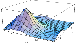
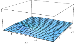
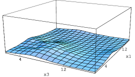
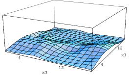
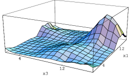
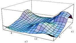
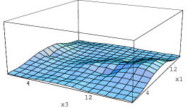
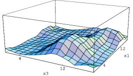
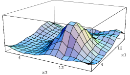
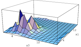
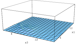
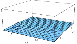
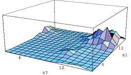
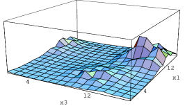
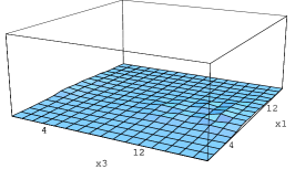
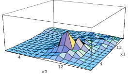
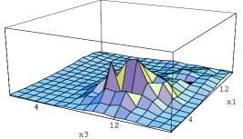
Figure 3: First three rows: the lowest Laplacian mode in a thermalized background with $\zeta=0.02$, $0.355$, $0.48$ from left to right and in lattice planes $(x_{2},x_{4})=(12,1),(4,4),(6,3)$ from first to third row (vertical scale 0.05). The last three rows show the corresponding profiles of the kinetic term (vertical scale 0.0025).

In this subsection we explore the Laplacian modes as an analyzing tool on thermalized gauge field configurations [4]. Fig. 3 shows the lowest-lying mode in a generic background obtained on a $16^{3}\cdot 4$ lattice at $\beta=2.2$ (which amounts to $T=0.75\,T_{c}$) confirming the expectation that these modes are free of UV fluctuations. The ‘evolution’ of the Laplacian mode with the angle $\zeta$ is shown horizontally in Fig. 3, while the first three rows represent different but fixed lattice planes, which contain the global maximum of the mode. In the example we find three lattice locations which become the global maximum within some $\zeta$-interval. Therefore, the lowest Laplacian mode in a thermalized background hops, too.

At the hopping points in $\zeta$ the value of the maximum as well as the inverse participation ratio (taking values between ${\rm IPR}\!=\!4$ and ${\rm IPR}\!=\!11$) decrease and the mode rearranges itself. For some boundary conditions the lowest Laplacian mode can be characterized as a global structure [4]. As the three last rows of Fig. 3 show, the kinetic term follows the modulus of the mode, but is less smooth.

Analyzing 50 independent configurations we found that the lowest mode hops up to four times as a function of $\zeta$. Apart from the Laplacian mode being wave-like, the hopping phenomenon resembles the behavior of the fermion zero mode in thermalized configurations [8]. However, in both cases it is not obvious which gluonic feature, e.g. in the topological charge, distinguishes the preferred locations. Interestingly, we have found a correlation of the maximum of the periodic and antiperiodic Laplacian mode to positive and negative Polyakov loops, respectively, see Fig. 4. This is the same tendency as for calorons (cf. Fig. 1) which could be understood as an argument in favor of calorons ‘underlying’ the quantum configurations. Alternatively, the Polyakov loop could play a role defining pinning centers for the Laplacian mode in the spirit of Anderson localization in a random potential [9].

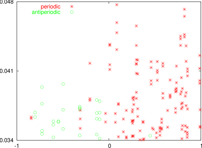
Figure 4: Scatterplots of the Polyakov loop (horizontal) at lattice sites where the modulus of the lowest Laplacian mode (vertical) is large: stars represent the periodic mode, circles the antiperiodic one.

The lowest Laplacian mode in the adjoint representation we have found to have minima at the caloron monopoles (see also [1, 10]) that extend to two-dimensional sheets for antiperiodic boundary conditions [4]. In thermalized backgrounds, the maxima of the adjoint modes are correlated to the fundamental ones with the same boundary condition, but are stronger localized than the latter.

3 A Fourier-like filter

Laplacian (‘harmonic’) eigenmodes can be used to define a new Fourier-like filter which we present now [4]. We were inspired by the representation of the field strength in terms of fermionic modes in [11], but here we aim to reconstruct directly the link variables on which any observable can be measured. To this end we combine the definition of the lattice Laplacian, Eq. (1), with a spectral decomposition and at $y=x+\hat{\mu}$ immediately obtain

$$U_{\mu}^{ab}(x) \!\!\!\!= \!\!\!\!-\sum_{n=1}^{\mathcal{N}}\lambda_{n}\phi^{a}_{n}(x)\phi^{*b}_{n}(x+\hat{\mu})\,,$$ (4)

$$\mathcal{N}=N_{1}N_{2}N_{3}N_{4}\cdot 2\,.$$

The idea is to truncate the sum on the right hand side of this equation at a small mode number $N$ compared to their total number $\mathcal{N}$.

The question arises, how to relate such an expression to a unitary link variable. Here the charge conjugation helps, since it guarantees that every eigenvalue is two-fold degenerate with eigenfunctions related as $\phi^{\prime a}(x)=\epsilon^{ab}\phi^{*b}(x)$. The corresponding bilinear expressions in Eq. (4) add up to an element of $SU(2)$ up to a factor. Such a situation is familiar from the staple average in cooling or smearing. We divide by the square root of this factor, which is the determinant and positive for all practical purposes, and obtain the final filter formula

$$\tilde{U}_{\mu}^{ab}(x)_{N}=(-\sum_{n=1}^{N}\lambda_{n}[\phi^{a}_{n}(x)\phi^{*b}_{n}(x+\hat{\mu})-$$

$$\epsilon^{ac}\phi^{*c}_{n}(x)\phi^{d}_{n}(x+\hat{\mu})\epsilon^{db}\,])/\sqrt{\det(\ldots)}\,.$$ (5)

The quality of the filter is controlled by $N$, where $N\!\!=\!\cal{N}$ reproduces the original configuration exactly. In the other extreme case, $N\!=\!1$, the filtered links $\tilde{U}_{\mu}(x)$ can be shown to be pure gauge. From the behavior of $\phi(x)$ under gauge transformations it follows immediately that $\tilde{U}_{\mu}(x)$ transforms as a link (and no gauge fixing is involved in the filter).

The filtering can be performed with Laplacian modes of any boundary condition. Then Eq. (5) is just the average over opposite boundary conditions $\zeta$ and $-\zeta$. This additional parameter $\zeta$ completely fixes the Polyakov loop at $N=1$ to ${\rm tr}\,\tilde{\mathcal{P}}(\vec{x})/2=\cos(2\pi\zeta)$, while for nontrivial cases $N\geq 2$ the Polyakov loop is observed to fluctuate around this value. It follows that in order to optimize the filter for our circumstances (confined phase, nontrivial holonomy calorons) the best choice is the intermediate case $\zeta=1/4$.

In order to test the filter, we again start with a caloron (this time over $16^{3}\cdot 4$). The action and topological density as well as the Polyakov loop plotted in Fig. 5 show, that the filter with the number of modes as low as $N=4$ starts to reproduce the classical structures qualitatively, while for $N=150$ the agreement is almost perfect.

During the filtering we have recorded the determinant used in Eq. (5) to project to an $SU(2)$-element. With increasing number $N$ of modes it increases, too (i.e. becomes closer to 1). Moreover, its variation over the lattice decreases, such that all links appear ‘equally well filtered’.

Figure 5: Action and topological density and Polyakov loop of a large caloron on $16^{3}\cdot 4$, filtered with boundary condition $\zeta=1/4$. From top to bottom: $N=4$ modes (densities multiplied by a factor of 100), $N=150$ modes (factor 400) and the original configuration (factor 400).

Now we turn to the application of the filter to thermalized configurations (at finite temperature), first by the example of Sect. 2.2.

Figure 6: Correlation of link variable components ${\rm tr}\,U_{\mu}(x)/2$ and ${\rm tr}\,U_{\mu}(x)\tau_{i}/2i$ ($\tau_{i}$ the Pauli matrices) between the original configuration and the filtered one with $N=2$ (left) and $N=100$ (middle) and within filtered links with $N=2$ vs. $N=4$ (right). In order not to overload the plots, only 2000 link variable components have been plotted.

The first question we want to address is the correlation of the filtered links to the original ones. Fig. 6 shows scatterplots including all $SU(2)$-components of the links in all $\mu$-directions and over all lattice locations. To compare link variables themselves makes sense, since the original and the filtered configuration come in the same gauge (in other words the application of the filter commutes with gauge transformations). Fig. 6 (left) shows that even in the first nontrivial case $N=2$ the filtered links are correlated to the original ones. With increasing number of involved modes this correlation becomes stronger as expected: in the scatterplot for $N=100$ (Fig. 6 (middle)) the deviation from the diagonal decreased compared to $N=2$. One can make this statement quantitative by computing the average square distance from the diagonal, which indeed is smaller for bigger $N$. Actually, it also shows that the time-like links are less correlated than the space-like ones, especially when using the ‘inappropriate’ periodic boundary conditions. Finally, Fig. 6 (right) shows that the filter with comparable number of modes produces strongly correlated links.

What is even more remarkable is that the filter method preserves the string tension. We plot the logarithm of the Polyakov loop correlator measured on 50 configurations at $T=0.75\,T_{c}$ in Fig. 7 (left), both for the original one and the filtered ones with $N=2,\,10,\,100$. It reveals a clearly linear behavior with a slope reproducing the original one within 15%. The minimal number of modes, $N=2$, suffices for this behavior. We conclude that the confining properties of lattice gauge theory are captured by the lowest Laplacian modes.

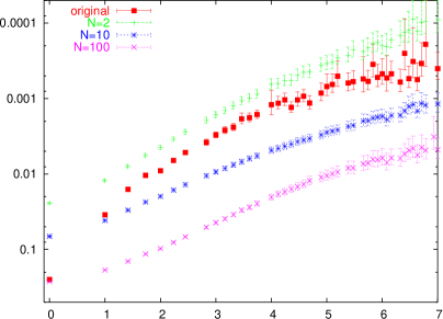
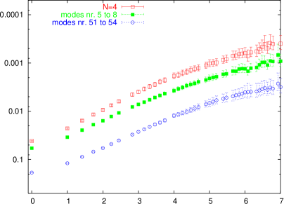
Figure 7: Polyakov loop correlators of 50 configurations at finite temperature, filtered with boundary condition $\zeta=1/4$ and plotted on an inverse logarithmic scale over the distance. Left: the original configurations vs. the filtered ones with $N=2,\,10,\,100$ modes. Right: 4 modes with various shifts in the ordinal number of the modes.

This property actually does not depend much on the ordinal number of the modes, see Fig. 7 (right). First of all, one can include the $N$ highest Laplacian modes. Due to the symmetry [3]

$$\phi_{\mathcal{N}-n}=(-1)^{\sum_{\mu}x_{\mu}}\phi_{n}\,,\quad\lambda_{\mathcal{N}-n}=16-\lambda_{n}\,,$$ (6)

including these highest modes results in the same bilinear contributions in Eq. (5) with the only modification $\lambda_{n}\rightarrow 16-2\lambda_{n}$. The Polyakov loop correlator computed from the 50 configurations filtered in this way agrees very well with the one discussed so far (and is therefore not shown in Fig. 7). The second possibility is to shift the mode number from 1 till 4 to say 5 till 8 or 51 till 54. The corresponding curves shown in Fig. 7 (right) reveal the same linear behavior up to a vertical shift. The Polyakov loop correlator is robust also against a third option, namely replacing the eigenvalues $\lambda_{n}$ in Eq. (5) by a constant, which again produces identical curves (not shown).

After filtering the Polyakov loop correlator has no sign of a Coulomb regime, since the filter has washed out short range fluctuations. At zero distance the values $\langle({\rm tr}\,\tilde{\mathcal{P}}(\vec{x}))^{2}\rangle$ are smaller than the original one. This reflects the already mentioned effect that the filtered links for small $N$ are mostly traceless (governed by the choice $\zeta=1/4$). The site distribution of the Polyakov loop is a narrow one around ${\rm tr}\,\tilde{\mathcal{P}}=0$ for $N=2$, but for $N=100$ is compatible with the original distribution which in turn is described by the Haar measure. Fig. 8 shows locally (for the example configuration and in a fixed lattice plane) that with growing $N$ more and more fluctuations appear in the Polyakov loop. Studies are under way to clarify whether the new filter method preserves other infrared features, like the spatial Wilson loops, and how it behaves at zero temperature.

Since the filter preserves the string tension from Polyakov loop correlators and is not biased to classical solutions nor to particular degrees of freedom in the gauge field (like monopoles or vortices), it is interesting to have a closer look at the vacuum structures that emerge when the filter is applied to generic configurations.

Concerning the action density, these objects are found to be isolated peaks (which are non-static and not necessarily (anti)selfdual). This phenomenon seems counterintuitive as the filter uses the lowest-lying Laplacian modes which are smooth. However, too small action density lumps have also been observed when filtering smooth calorons at low $N$ (cf. Fig. 5 (top)). This phenomenon presumably comes from the nonlinearity in the filter formalism (Eq. (5)), in particular the determinant used to scale up the mode contributions to an $SU(2)$-element. Interestingly, we have found a correlation of the peak structure of the filtered action density to that emerging after cooling or smearing in an early stage.

We stress that, in contrast to e.g. cooling, the filter does not involve the plaquette action and thus is not made to reduce it in the first place. Upon filtering the links, the total action does become smaller, but only down to some amount (in our example down to 66 instanton units at $N=2$), which might well be the minimal content necessary to reproduce the infrared physics. More work has to be done to better understand the spiky structures induced by the filter.

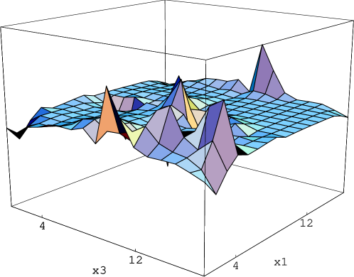
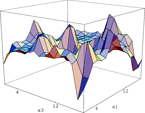
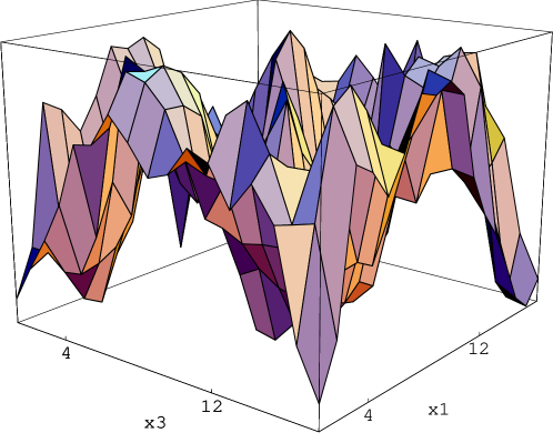
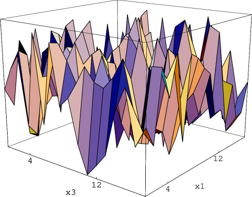
Figure 8: Polyakov loop ‘evolution’ with increasing number of modes for the thermalized example in a fixed lattice plane ($x_{2}=6$). From top to bottom: $N=2,\,10,\,100$ and the original configuration. The vertical axes are from $-1$ to $1$.

References

- [1] F. Bruckmann, T. Heinzl, T. Vekua, and A. Wipf, Magnetic monopoles vs. Hopf defects in the Laplacian (Abelian) gauge, Nucl. Phys. B593 (2001) 545–561, [hep-th/0007119].
- [2] P. de Forcrand and M. Pepe, Laplacian gauge and instantons, Nucl. Phys. Proc. Suppl. 2001 (1994) 498–501, [hep-lat/0010093].
- [3] J. Greensite, Š. Olejník, M. I. Polikarpov, S. N. Syritsyn, and V. I. Zakharov, Localized eigenmodes of covariant Laplacians in the Yang-Mills vacuum, Phys. Rev. D71 (2005) 114507, [hep-lat/0504008].
- [4] F. Bruckmann and E.-M. Ilgenfritz, Laplacian modes probing gauge fields, Phys. Rev. D (in print), hep-lat/0509020.
- [5] T. C. Kraan and P. van Baal, Periodic instantons with non-trivial holonomy, Nucl. Phys. B533 (1998) 627–659, [hep-th/9805168].
- [6] K. Lee and C. Lu, calorons and magnetic monopoles, Phys. Rev. D58 (1998) 025011, [hep-th/9802108].
- [7] M. García Pérez, A. González-Arroyo, C. Pena, and P. van Baal, Weyl-Dirac zero-mode for calorons, Phys. Rev. D60 (1999) 031901, [hep-th/9905016].
- [8] C. Gattringer and S. Schaefer, New findings for topological excitations in SU(3) lattice gauge theory, Nucl. Phys. B654 (2003) 30–60, [hep-lat/0212029].
- [9] P. W. Anderson, Absence of diffusion in certain random lattices, Phys. Rev. 109 (1958) 1492.
- [10] C. Alexandrou, M. D’Elia, and P. de Forcrand, The relevance of center vortices, Nucl. Phys. Proc. Suppl. 83 (2000) 437–439, [hep-lat/9907028].
- [11] C. Gattringer, Testing the self-duality of topological lumps in SU(3) lattice gauge theory, Phys. Rev. Lett. 88 (2002) 221601, [hep-lat/0202002].