QCD at High Temperature :
Results from Lattice Simulations with an Imaginary $\mu$

Abstract

We summarize our results on the phase diagram of QCD with emphasis on the high temperature regime. For $T\geq 1.5T_{c}$ the results are compatible with a free field behavior, while for $T\simeq 1.1T_{c}$ this is not the case, clearly exposing the strongly interacting nature of QCD in this region.

1 Introduction

The historical developments of the phase diagram of QCD is characterized by an increasing complication: according to early views based on a straightforward application of asymptotic freedom , the phase diagram was sharply divided into an hadronic phase and a quark gluon plasma phase. In the late 90’s it was appreciated that the high density region is much more complicated than previously thought Alford . In the last couple of years, it was the turn of the region above $T_{c}$ to become more rich: the survival of bound states above the phase transition brought up the idea of a more complicated, highly non–perturbative phase, whose precise nature has not been clarified yetsQGP . The properties of the high temperature phase are especially interesting in view of the ongoing ultrarelativistic heavy ions collisions experiments with at RHIC, which explore temperatures close to $T_{c}$, and of the future experiments at LHC, which will approach the perturbative, free gas limit of QCD.

Up to which extent the properties of the matter produced in these ultrarelativistic heavy ion collisions can be predicted by the basic theory of strong interactions, Quantum Chromo Dynamics? In this note we review our results D'Elia:2002gd ; D'Elia:2004at ; progress on this point,

QuantumChromoDynamics (QCD) basic degrees of freedom are quarks and gluons. The Lagrangian built by use of these fundamental fields enjoys local and (approximate) global symmetries. The realization of the global chiral symmetry depends on the thermodynamic conditions of the system : it is spontaneously broken, with the accompanying phenomena of Goldstone modes and a mass gap, in ordinary conditions, and it gets restored at high temperature. At the same time, confinement, which is realized in the normal phase, disappears at high temperature: all in all, in our low temperature world quarks are confined within hadrons, there are light preudoscalar mesons, the Goldstone bosons, and there are massive mesons and baryons. In the high temperature phase - the Quark Gluon Plasma - quarks and gluons are no longer confined, and the mass spectrum reflects the symmetries of the Lagrangian.

In a standard nuclear physics approach these features of the two phases are imposed by fiat, and the phase transition is obtained by equating the free energies of the quark-gluon gas on one side, and the hadron gas on the other side of the transition. At a variance with this, an approach based on QCD derives the different degrees of freedom of the two phases, as well as the phase transition line, from the same Lagrangian. These calculations, being completely non–perturbative, require a specific technique, Lattice QCD.

2 Lattice QCD Thermodynamics

Without entering into the details of this approach lat , let us just remind that the QCD equations are put on a ’grid’ which should be fine enough to resolve details, and large enough to accommodate hadrons within: obviously, this would call for grids with a large number of points. On the other hand, the calculations complexity grows fast with the number of nodes in the grid, and the actual choices rely on a compromise between physics requirements and computer capabilitiestilo .

In practical numerical approaches, the lattice discretization is combined with a statistical techniques for the computation of the physical observables. This requires a positive ’measure’, which is given by the exponential of the Action. A notorious problem plagues these calculations at finite baryon density, as the Action itself becomes complex, with a non–positive definite real part: because of this, for many years QCD at nonzero baryon density was not progressing at all.

Luckily, in the last four years a few lattice techniques – imaginary chemical potential, Taylor expansion, multiparameter reweighting – proven successful for $\mu_{B}/T<1.$ uno ; due ; FoPh ; D'Elia:2002gd ; D'Elia:2004at ; tre ; susc . It has to be stressed, however, that these techniques are just dodges and workaround, and do not provide a real solution to the ’sign problem’. Moreover, due to the computer limitations sketched above, which we hope will be soon overcome by the next generation of supercomputers tilo , the results have not yet reached the continuum, infinite volume limit.

While waiting for final results in the scaling limit and with physical values of the parameters, it is very useful to contrast and compare current lattice results with model calculations and perturbative studies. The imaginary chemical potential approachLombardo:1999cz ; Hart:2000ef ; FoPh ; D'Elia:2002gd ; D'Elia:2004at ; Giudice:2004se to QCD thermodynamics seems to be ideally suited for the interpretation and comparison with analytic results. Results from an imaginary $\mu$ have been obtained for the critical line of the two, three and two plus one flavor model FoPh , as well as for four flavor D'Elia:2002gd . Thermodynamics results – order parameter, pressure, number density – were obtained for the four flavor model D'Elia:2004at , and are extended in this note, where we concentrate on the region $T>T_{c}$.

Figure 1: Sketch of the phase diagram in the $\mu^{2},T$ plane: the solid line is the chiral transition, the dashed line is the Roberge Weiss transition Roberge:1986mm , the dotted line the $\mu^{2}=0$ axis. Simulations can be carried out at $\mu^{2}\leq 0$ and results continued to the physical domain $\mu^{2}\geq 0$. The derivative and reweighting methods have been used so far to extract informations from simulations performed at $\mu=0.$ The imaginary chemical potential approaches uses results on the left hand half plane. Different methods could be combined to improve the overall performance.

3 Imaginary Chemical Potential

The imaginary chemical potential method uses information from all of the negative $\mu^{2}$ half plane (Fig. 1) to explore the positive, physical relevant region.

The main physical idea behind any practical application is that at $\mu=0$ fluctuations allow the exploration of $N_{b}\neq 0$ hence tell us about $\mu\neq 0$. Mutatis mutandis, this is the same condition for the reweighting methods to be effective: the physics of the simulation ensemble has to overlap with that of the target ensemble.

A practical way to use the results obtained at negative $\mu^{2}$ relies on their analytical continuation in the real plane. For this to be effectiveLombardo:1999cz ${\cal Z}(\mu,T)$ must be analytical, nontrivial, and fulfilling:

$$\chi(T,\mu)=\partial\rho(\mu,T)/\partial\mu=\partial^{2}logZ(\mu,T)/\partial\mu^{2}>0$$ (1)

This approach has been tested in the strong coupling limit Lombardo:1999cz of QCD, in the dimensionally reduced model of high temperature QCD Hart:2000ef and, more recently, in the two color model Giudice:2004se .

4 The Hot Phase and the approach to a Free Gas

At high temperature, in the weak coupling regime, finite temperature perturbation theory might serve as a guidance, suggesting that the first few terms of the Taylor expansion might be adequate in a wider range of chemical potentials. So, at a variance with the expansion in the hadronic phase, where the natural parametrization is given by a Fourier analysisD'Elia:2002gd ; D'Elia:2004at , in this phase the natural parametrization for the grand partition function is a polynomial.

The leading order result for the pressure $P(T,\mu)$ in the massless limit is easily computed, given that at zero coupling the massless theory reduces to a non–interacting gas of quarks and gluons, yielding for the pressure

$$p(T,\mu)=\frac{\pi^{2}}{45}T^{4}\left(8+7N_{c}\frac{n_{f}}{4}\right)+\frac{n_{f}}{2}\mu^{2}T^{2}+\frac{n_{f}}{4\pi^{2}}\mu^{4}\,.$$ (2)

Obviously, when analytically continued to the negative $\mu^{2}$ side, this gives

$$p(T,\mu_{I})=\frac{\pi^{2}}{45}T^{4}\left(8+7N_{c}\frac{n_{f}}{4}\right)-\frac{n_{f}}{2}\mu_{I}^{2}T^{2}+\frac{n_{f}}{4\pi^{2}}\mu_{I}^{4}\,.$$ (3)

Because of the Roberge Weiss Roberge:1986mm periodicity this polynomial behavior should be cut at the Roberge Weiss transition $\mu_{I}=\pi T/3$: this is consistent with the Roberge Weiss critical line being strongly first order at high temperature. We discuss first the results of the fits of the number density to polynomial form; then we contrast these results with a free field behavior.

The considerations above suggests a natural ansatz for the behavior of the number density in this phase as a simple polynomial with only odd powers. We performed then fits to

$$n(T,\mu_{I})=ia(T)\mu_{I}-ib(T)\mu_{I}^{3}$$ (4)

whose obvious analytic continuation is

$$n(T,\mu)=a(T)\mu+b(T)\mu^{3}\,.$$ (5)

Note again that $a(T)=\chi_{q}(T,\mu=0)$.

In ref. D'Elia:2004at we contrasted the results for the particle number at $T=1.5T_{c}$, $T=2.5T_{c}$, $T=3.5T_{c}$ with a free field behaviour.

Some deviations are apparent, whose origin we would like to understand. It would be however arduous, given the strong lattice artifacts, to try to make contact with a rigorous perturbative analysis carried out in the continuum Vuorinen:2004rd ; Vuorinen:2003fs ; Ipp:2003yz . Rather then attempting that, we parametrize the deviation from a free field behavior as Szabo:2003kg ; Letessier:2003uj

$$\Delta P(T,\mu)=f(T,\mu)P^{L}_{free}(T,\mu)$$ (6)

where $P^{L}_{free}(T,\mu)$ is the lattice free result for the pressure. For instance, in the discussion of Ref. Letessier:2003uj

$$f(T,\mu)=2(1-2\alpha_{s}/\pi)$$ (7)

and the crucial point was that $\alpha_{s}$ is $\mu$ dependent.

We can search for such a non trivial prefactor $f(T,\mu)$ by taking the ratio between the numerical data and the lattice free field result $n^{L}_{free}(\mu_{I})$ at imaginary chemical potential:

$$R(T,\mu_{I})=\frac{n(T,\mu_{I})}{n^{L}_{free}(\mu_{I})}$$ (8)

A non-trivial (i.e. not a constant) $R(T,\mu_{I})$ would indicate a non-trivial $f(T,\mu)$.

We found that $R(T,\mu_{i})$ is constant within errors, so that our data do not permit to distinguish a non trivial factor within the error bars: rather, the results for $T\geq 1.5T_{c}$ seem consistent with a free lattice gas, with an fixed effective number of flavors $N^{eff}_{f}(T)/4=R(T)$: $N^{eff}_{f}=0.92\times 4$ for $T=3.5T_{c}$, and $N^{eff}_{f}=0.89\times 4$ for $T=1.5T_{c}$.

One last remark concerns the mass dependence of the results, which, as in the broken phase, can be computed from the derivative of the chiral condensate. In the chiral limit this gives $\frac{\partial n}{\partial m}=0$ , since the chiral condensate is identically zero. We have verified that $\frac{\partial n}{\partial m}$ remains very small compared to $n$ itself: in a nutshell, in the quark gluon plasma phase $<\bar{\psi}\psi>$ is very small (zero in the chiral limit), while the number density grows larger, and this implies that the mass sensitivity is greatly reduced with respect to that in the broken phase.

The discussions presented above bring very naturally to the consideration of a dynamical region which is comprised between the deconfinement transition, and the endpoint of the Roberge Weiss transition.

In this dynamical region the analytic continuation is valid till $\mu=\infty$ along the real axis, since there are no singularities for real values of the chemical potential. The interval accessible to the simulations at imaginary $\mu$ is small, as simulations in this area hits the chiral critical line for $\mu^{2}<0$.

This region is of special interest and it is here that we are concentrating our efforts: In Fig. 2 we show our new results obtained at $T/T_{c}=1.095$, indicating a non trivial deviation from a free field behaviour.

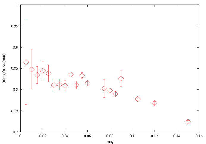
Figure 2: The ratio of the lattice results to the free fields results $R(T,\mu_{I})$ at $T\simeq 1.1T_{c}$ : an horizontal line would indicate a nearly–free behaviour which is clearly incompatible with the data. At this temperature the chiral transition takes place at imaginary chemical potential , i.e. at a negative $\mu^{2}$ (Fig.1)

.

Let us make some general consideration about the thermodynamic behavior in this region by considering the critical line at imaginary chemical potential. Let us consider first the case of a second order transition: the analytic continuation of the polynomial predicted by perturbation theory for positive $\mu^{2}$ would hardly reproduce the correct critical behavior at the second order phase transition for $\mu^{2}<0$. In fact, for a second order chiral transition at negative $\mu^{2}$, $\Delta P(T,\mu^{2})\propto(\mu^{2}-{\mu^{2}}_{c})^{\chi}$, where $\chi$ is a generic exponent. As the window between the critical line and the $\mu=0$ axis is anyway small, such behavior - possibly with subcritical corrections - should persist in the proximity of the real axis. For generic values of the exponent a second order chiral transition seems incompatible with a free field behavior. The same discussion can be repeated for a first order transition of finite strength, by trading the critical point $\mu_{c}$ with the spinodal point $\mu^{*}$ . So deviations from free field are to be expected in this intermediate regime.

A more detailed discussion of these results, and their interrelation (or lack thereof) with a strongly interactive quark gluon plasma will be given elsewhere progress .

5 Future directions

The approach to a free gas of quarks and gluons is a fascinating subject: we are moving from a world of colorless hadrons to a world of colored particles - quarks, gluons, and perhaps many more.

Three different, independent methods which afford a quantitative approach to this problem have been proposed and exploited in the past few years, producing several interesting and coherent results. In particular we have focussed on the properties of the hot phase right above the critical temperature, where we have observed a clear non–perturbative behaviour for the thermodyamical observables, showing that the system is still very far from a free gas of quark gluons.

These results, however, still need improvement: in particular, small quark masses, and a controlled approach to the continuum limit. All this requires a large amount of computer resources, and there is hope that the new dedicated supercomputers for lattice QCD - QCDOC and apeNEXT - will produce significant advances in this field.

High quality numerical results together with a careful consideration of phenomenological models and critical behaviour in the negative $\mu^{2}$ half–plane should produce a coherent and complete description of the high temperature phase of the strong interactions, which will hopefully confront soon ongoing and future experiments.

References

- (1) M. Alford, this volume.
- (2) E. V. Shuryak and I. Zahed, Phys. Rev. C 70, 021901 (2004); F. Karsch, S. Ejiri and K. Redlich, arXiv:hep-ph/0510126.
- (3) see e.g. J. Smit, Cambridge Lect. Notes Phys. 15 (2002) 1.
- (4) M. D’Elia and M. P. Lombardo, Phys. Rev. D 67 (2003) 014505.
- (5) M. D’Elia and M. P. Lombardo, Phys. Rev. D 70 (2004) 074509.
- (6) M. D’Elia, F. Di Renzo and M.P. Lombardo, work in progress.
- (7) T. Wettig, talk at Lattice2005, Dublin, to appear in the Proceedings.
-
(8)
Z. Fodor and S. D. Katz,
Phys. Lett. B 534 (2002) 84;
JHEP 0404 (2004) 50;
Z. Fodor, S. D. Katz and K. K. Szabo, Phys. Lett. B 568 (2003) 73;
F. Csikor et al. JHEP 0405 (2004) 046;
S. D. Katz, Nucl. Phys. Proc. Suppl. 129 (2004) 60. - (9) Ph. de Forcrand et al., Nucl. Phys. Proc. Suppl. 119 (2003) 541.
-
(10)
Ph. de Forcrand and O. Philipsen,
Nucl. Phys. B 642 (2002) 290;
Nucl. Phys. B 673 (2003) 170. -
(11)
C. R. Allton et al.,
Phys. Rev. D 66 (2002) 067801;
Phys. Rev. D 68, (2003) 014081. - (12) R. Gavai, S. Gupta and R. Roy, Prog. Theor. Phys. Suppl.153 (2004) 270. .
- (13) A. Roberge and N. Weiss, Nucl. Phys. B 275, 734 (1986).
- (14) M. P. Lombardo, Nucl. Phys. Proc. Suppl. 83, 375 (2000).
- (15) A. Hart, M. Laine and O. Philipsen, Phys. Lett. B 505, 141 (2001).
- (16) P. Giudice and A. Papa, Phys. Rev. D 69, 094509 (2004).
- (17) K. K. Szabo and A. I. Toth, JHEP 0306, 008 (2003).
- (18) F. Csikor, G. I. Egri, Z. Fodor, S. D. Katz, K. K. Szabo and A. I. Toth, Prog. Theor. Phys. Suppl. 153, 93 (2004).
- (19) J. Letessier and J. Rafelski, Phys. Rev. C 67, 031902 (2003).
- (20) A. Vuorinen, arXiv:hep-ph/0402242.
- (21) A. Vuorinen, Phys. Rev. D 68, 054017 (2003).
- (22) A. Ipp, A. Rebhan and A. Vuorinen, Phys. Rev. D 69, 077901 (2004).