Möbius Fermions

Abstract

We introduce a new domain wall operator that represents a full (real) Möbius transformation of a given non-chiral Dirac kernel. Shamir’s and Chiu/Boriçi’s domain wall fermions are special cases of this new class. By tuning the parameters of the Möbius operator and by introducing a new Red/Black preconditioning, we are able to reduce the computational effort substantially.

1 Introduction

The key idea in evading the Nielsen-Ninomiya no-go theorem [1, 2], which forbade the construction of lattice fermion actions with chiral symmetry under rather general conditions, was introduced by Kaplan [3]. In his construction four dimensional chiral zero modes appeared as bound states on a mass defect or 3-brane in a five dimensional theory. Much like the work of Callan and Harvey [4] in the continuum, anomalous currents in the 4 dimensional theory are understood as the flow on or off the mass defect of conserved 5 dimensional currents. This work led to two concrete realizations of lattice fermions with chiral symmetry. The domain wall fermions [5, 6, 7, 8] and the overlap fermions [9, 10, 11, 12, 13].

Here we introduce the Möbius domain wall operator, a generalization of Shamir’s and Chiu/Boriçi’s suggestions. It is given by (to keep the notation simple, we choose the length of the fifth domain wall dimension $L_{s}$ equal to 4)

$$D_{DW}(m)=\hskip 56.9055pt$$ (1)

$$\left(\begin{array}[]{cccc}\hskip-3.69899ptD^{(1)}_{+}&\hskip-3.69899ptD^{(1)}_{-}P_{-}&\hskip-3.69899pt0&\hskip-3.69899pt-mD^{(1)}_{-}P_{+}\\ \hskip-3.69899ptD^{(2)}_{-}P_{+}&\hskip-3.69899ptD^{(2)}_{+}&\hskip-3.69899ptD^{(2)}_{-}P_{-}&\hskip-3.69899pt0\\ \hskip-3.69899pt0&\hskip-3.69899ptD^{(3)}_{-}P_{+}&\hskip-3.69899ptD^{(3)}_{+}&\hskip-3.69899ptD^{(3)}_{-}P_{-}\\ \hskip-3.69899pt-mD^{(4)}_{-}P_{-}&\hskip-3.69899pt0&\hskip-3.69899ptD^{(4)}_{-}P_{+}&\hskip-3.69899ptD^{(4)}_{+}\\ \end{array}\hskip-3.69899pt\right)\hskip-10.81218pt$$ (6)

with

$$D^{(i)}_{+} = b_{i}D_{w}+1,\;\;\;D^{(i)}_{-}=c_{i}D_{w}-1,$$ (7)

$$P_{+} = \frac{1}{2}(1+\gamma_{5}),\;\;\;P_{-}=\frac{1}{2}(1-\gamma_{5}).$$ (8)

$D_{w}$ denotes the Wilson Dirac matrix

$$D_{w}(M_{5})=(4+M_{5})\delta_{x,y}-\frac{1}{2}\bigl{[}(1-\gamma_{\mu})$$ (9)

$$U_{\mu}(x)\delta_{x+\mu,y}+(1+\gamma_{\mu})U_{\mu}^{\dagger}(y)\delta_{x,y+\mu}\bigr{]}.$$

Note, that this choice is not mandatory, but that any other Dirac operator could have been used here as well.

Eq.(1) is a generic expression for the domain wall fermions. The different operators, Shamir, Chiu/Boriçi and Möbius, are characterized by the coefficients $b_{i},c_{i}$ in eq.(7). The Möbius operator contains Shamir’s and Chiu/Boriçi’s suggestions as special cases. For Möbius, the coefficients are only constrained to be:

• $b_{i},c_{i}\;\in\;\Re$ ,

• $b_{i}-c_{i}=const,\;\forall\;i\;\in\;L_{s}$ (i.e. $const$ is independent of $i$).

Shamir and Chiu/Boriçi use:

$$\begin{array}[]{ccc}\mbox{Shamir:}&b_{i}=a,&c_{i}=0,\\ \mbox{Bori\c{c}i:}&b_{i}=a,&c_{i}=a,\\ \mbox{Chiu:}&b_{i}=a_{i},&c_{i}=a_{i}.\end{array}$$ (13)

with $a,a_{i}\;\in\;\Re.$

To understand the meaning of the coefficients, we will translate the 5 dimensional domain fermions into a 4 dimensional overlap operator. This is done via a linear matrix transformation.

2 Domain wall - overlap transformation

The domain wall and the overlap operator are connected through a linear matrix transformation [14, 15, 16]. The length of the fifth domain wall dimension corresponds to the order of a polynomial, that approximates the sign function on the overlap side. Accordingly, domain wall fermions can be seen as a preconditioning of the overlap operator.

In the following, $D_{DW}$ will denote the generic domain wall operator and $L_{s}$ the length of the fifth domain wall dimension. Here we will choose $L_{s}=4$ to keep the notation simple, but all formulas hold for any $L_{s}$. $D_{OV}$ will denote the approximation to the overlap operator, as defined through the polynomial of finite order, that describes the sign function.

The domain wall - overlap transformation reads:

$$L\;D_{DW}(m)\;R\;=\;F\;D^{5}_{OV}(m),$$ (14)

with

$$F\;=L\;D_{DW}(1)\;R,$$ (15)

$$L=\left(\begin{array}[]{cccc}1&S_{1}&S_{1}S_{2}&S_{1}S_{2}S_{3}\\ 0&1&S_{2}&S_{2}S_{3}\\ 0&0&1&S_{3}\\ 0&0&0&1\end{array}\right)\times$$ (20)

$$\left(\begin{array}[]{cccc}{Q_{-}^{(1)}}^{-1}&0&0&0\\ 0&{Q_{-}^{(2)}}^{-1}&0&0\\ 0&0&{Q_{-}^{(3)}}^{-1}&0\\ 0&0&0&{Q_{-}^{(4)}}^{-1}\\ \end{array}\right)\gamma_{5},$$ (25)

$$R=P\hat{R}=\hskip 65.44142pt$$ (26)

$$\left(\begin{array}[]{cccc}\hskip-3.69899ptP_{-}&\hskip-3.69899ptP_{+}&\hskip-3.69899pt0&\hskip-3.69899pt0\\ \hskip-3.69899pt0&\hskip-3.69899ptP_{-}&\hskip-3.69899ptP_{+}&\hskip-3.69899pt0\\ \hskip-3.69899pt0&\hskip-3.69899pt0&\hskip-3.69899ptP_{-}&\hskip-3.69899ptP_{+}\\ \hskip-3.69899ptP_{+}&\hskip-3.69899pt0&\hskip-3.69899pt0&\hskip-3.69899ptP_{-}\\ \end{array}\right)\hskip-3.69899pt\left(\begin{array}[]{cccc}\hskip-3.69899pt-1&\hskip-3.69899pt0&\hskip-3.69899pt0&\hskip-3.69899pt0\\ \hskip-3.69899pt-S_{2}S_{3}S_{4}\,d&\hskip-3.69899pt1&\hskip-3.69899pt0&\hskip-3.69899pt0\\ \hskip-3.69899pt-S_{3}S_{4}\,d&\hskip-3.69899pt0&\hskip-3.69899pt1&\hskip-3.69899pt0\\ \hskip-3.69899pt-S_{4}\,d&\hskip-3.69899pt0&\hskip-3.69899pt0&\hskip-3.69899pt1\\ \end{array}\right),\hskip-10.81218pt$$ (35)

$$D^{5}_{OV}(m)=\left(\begin{array}[]{cccc}D_{OV}(m)&0&0&0\\ 0&1&0&0\\ 0&0&1&0\\ 0&0&0&1\\ \end{array}\right).$$ (40)

The matrix entries are defined as follows:

$$Q^{(i)}_{+} = \gamma_{5}D_{w}(b_{i}P_{+}+c_{i}P_{-})+1,$$ (41)

$$Q^{(i)}_{-} = \gamma_{5}D_{w}(b_{i}P_{-}+c_{i}P_{+})-1,$$ (42)

$$S_{i} = T_{i}^{-1}=-(Q_{-}^{(i)})^{-1}Q_{+}^{(i)},$$ (43)

$$d = P_{+}-mP_{-}.$$ (44)

$T_{i}^{-1}$ is called the transfer matrix.

Multiplying the matrices on the left hand side of eq.(14) (multiply first by $P$, then $L$ and $\hat{R}$, where it might be useful to remember that $(bP_{-}+cP_{+})^{-1}=\frac{1}{b}P_{-}+\frac{1}{c}P_{+}$) leads to the entry $[LD_{DW}(m)R]_{11}=-(P_{-}-mP_{+})+S(P_{+}-mP_{-})$, or

$$F=\left(\begin{array}[]{cccc}(S+1)\gamma_{5}&0&0&0\\ 0&1&0&0\\ 0&0&1&0\\ 0&0&0&1\\ \end{array}\right)$$ (49)

and

$$D_{OV}(m)=\frac{1}{2}\left(1+m+(1-m)\gamma_{5}\frac{(S-1)}{(S+1)}\right),$$ (50)

with $S=S_{1}S_{2}S_{3}S_{4}$ (note, that the fact that there are four factors $S_{1},\cdots,S_{4}$ is due to our choice $L_{s}=4$). If ${(S-1)}/{(S+1)}$ was an approximation to the sign function, eq.(50) would be the corresponding approximation to the overlap operator. To see whether there is such a relation, we define $H^{(i)}_{T}$ through:

$$S_{i}=\frac{H^{(i)}_{T}+1}{H^{(i)}_{T}-1},$$ (51)

i.e.

$$H^{(i)}_{T}=(b_{i}+c_{i})\gamma_{5}D_{w}\frac{1}{2+(b_{i}-c_{i})D_{w}}.$$ (52)

We define the kernel $H_{T}$ as

$$H_{T}=\gamma_{5}D_{w}\frac{1}{2+(b_{i}-c_{i})D_{w}},$$ (53)

i.e.

$$H^{(i)}_{T}=(b_{i}+c_{i})H_{T}.$$ (54)

This leads to

$$\frac{(S-1)}{(S+1)}=\frac{A-B}{A+B},$$ (55)

with

$$A=(H^{(1)}_{T}\hskip-1.42271pt+\hskip-1.42271pt1)(H^{(2)}_{T}\hskip-1.42271pt+\hskip-1.42271pt1)(H^{(3)}_{T}\hskip-1.42271pt+\hskip-1.42271pt1)(H^{(4)}_{T}\hskip-1.42271pt+\hskip-1.42271pt1),$$ (56)

$$B=(H^{(1)}_{T}\hskip-1.42271pt-\hskip-1.42271pt1)(H^{(2)}_{T}\hskip-1.42271pt-\hskip-1.42271pt1)(H^{(3)}_{T}\hskip-1.42271pt-\hskip-1.42271pt1)(H^{(4)}_{T}\hskip-1.42271pt-\hskip-1.42271pt1).$$ (57)

One can choose the coefficients $b_{i}$ and $c_{i}$ such that eq.(55) corresponds to an approximation $\epsilon$ to the sign function with kernel $H_{T}$. As mentioned above, we set $b_{i}-c_{i}$ equal to a constant value for all $i$, i.e. the denominator is independent of $i$.

Possible polynomial approximations are:

• $c_{i}+b_{i}=const,\;\forall\;i\;\in\;L_{s}$. This corresponds to Neuberger’s polar decomposition.

• $c_{i}+b_{i}$ equal to Zolotarev’s coefficients [8].

We can summarize this findings as

$$D_{OV}(m)=\frac{1}{2}\left(1+m+(1-m)\;\gamma_{5}\;\epsilon(H_{T})\right).$$ (58)

3 Domain Wall preconditioning

Here we will describe how the quark propagator can be determined via the 5 dimensional domain wall operator.

We are interested in the 4 dimensional propagator $x_{1}$ (corresponding to the source b), given by

$$D_{OV}x_{1}=b.$$ (59)

Eq.(14) can be used to precondition eq.(59). As it stands, eq.(14) is not suitable for this task. We therefore perform the following simplifications:

• Multiply eq.(14) by $F^{-1}$ from the left

  $$\hat{R}^{-1}P^{-1}D^{-1}_{DW}(1)D_{DW}(m)P\hat{R}=D_{OV},$$ (60)

• then multiply by $\hat{R}$ from the left and by $\hat{R}^{-1}$ from the right

  $$P^{-1}D^{-1}_{DW}(1)D_{DW}(m)P=\hat{R}D_{OV}\hat{R}^{-1}.$$ (61)

The right hand side of eq.(61) is then given by (with $d=P_{+}-mP_{-}$)

$$\hat{R}D_{OV}\hat{R}^{-1}\hskip-3.98337pt=\hskip-3.98337pt\left(\begin{array}[]{cccc}\hskip-3.98337ptD_{OV}&\hskip-3.98337pt0&\hskip-3.98337pt0&\hskip-3.98337pt0\\ \hskip-3.98337ptS_{2}S_{3}S_{4}(D_{OV}\hskip-2.84544pt-\hskip-2.84544pt1)\,d&\hskip-3.98337pt1&\hskip-3.98337pt0&\hskip-3.98337pt0\\ \hskip-3.98337ptS_{3}S_{4}(D_{OV}\hskip-2.84544pt-\hskip-2.84544pt1)\,d&\hskip-3.98337pt0&\hskip-3.98337pt1&\hskip-3.98337pt0\\ \hskip-3.98337ptS_{4}(D_{OV}\hskip-2.84544pt-\hskip-2.84544pt1)\,d&\hskip-3.98337pt0&\hskip-3.98337pt0&\hskip-3.98337pt1\\ \end{array}\right).\hskip-10.81218pt$$ (66)

Obviously, with

$$\left(\begin{array}[]{cccc}\hskip-3.98337ptD_{OV}&\hskip-3.98337pt0&\hskip-3.98337pt0&\hskip-3.98337pt0\\ \hskip-3.98337ptS_{2}S_{3}S_{4}(D_{OV}\hskip-2.84544pt-\hskip-2.84544pt1)\,d&\hskip-3.98337pt1&\hskip-3.98337pt0&\hskip-3.98337pt0\\ \hskip-3.98337ptS_{3}S_{4}(D_{OV}\hskip-2.84544pt-\hskip-2.84544pt1)\,d&\hskip-3.98337pt0&\hskip-3.98337pt1&\hskip-3.98337pt0\\ \hskip-3.98337ptS_{4}(D_{OV}\hskip-2.84544pt-\hskip-2.84544pt1)\,d&\hskip-3.98337pt0&\hskip-3.98337pt0&\hskip-3.98337pt1\\ \end{array}\right)\hskip-5.69046pt\left(\begin{array}[]{c}\hskip-3.98337ptx_{1}\hskip-3.98337pt\\ \hskip-3.98337ptx_{2}\hskip-3.98337pt\\ \hskip-3.98337ptx_{3}\hskip-3.98337pt\\ \hskip-3.98337ptx_{4}\hskip-3.98337pt\\ \end{array}\right)\hskip-3.98337pt=\hskip-3.98337pt\left(\begin{array}[]{c}\hskip-3.98337ptb\hskip-3.98337pt\\ \hskip-3.98337pt0\hskip-3.98337pt\\ \hskip-3.98337pt0\hskip-3.98337pt\\ \hskip-3.98337pt0\hskip-3.98337pt\\ \end{array}\right)$$ (79)

$x_{1}$ is still the solution of $D_{OV}x_{1}=b$. Equivalently, we can find $x_{1}$ by solving the left hand side of eq.(61)

$$P^{-1}D^{-1}_{DW}(1)D_{DW}(m)P\left(\begin{array}[]{c}x_{1}\\ x_{2}\\ x_{3}\\ x_{4}\\ \end{array}\right)=\left(\begin{array}[]{c}b\\ 0\\ 0\\ 0\\ \end{array}\right)$$ (88)

or

$$D_{DW}(m)P\left(\begin{array}[]{c}x_{1}\\ x_{2}\\ x_{3}\\ x_{4}\\ \end{array}\right)=D_{DW}(1)P\left(\begin{array}[]{c}b\\ 0\\ 0\\ 0\\ \end{array}\right).$$ (97)

Typically, in linear system solvers, one iterates $D_{DW}(m)\vec{y}=\vec{b}$ alone, i.e. without the matrix $P$. Therefore, one has to reconstruct the real solution $x_{1}$ as

$$x_{1}=P_{-}y_{1}+P_{+}y_{4}.$$ (98)

This follows directly from $D_{DW}=D_{DW}PP^{-1}$, i.e $\vec{x}=P^{-1}\vec{y}$ .

4 The sign function

For later reference, we will state here a few simple properties of the sign function.

The sign function satisfies the following equation

$$\mbox{sign}(x)=\mbox{sign}(\lambda x),\;\forall\;x\;\in\;\Re\;,\;\lambda\;\in\;\Re^{+}.$$ (99)

Let $\epsilon$ be a polynomial approximation to the sign function. For $\epsilon$, eq.(99) doesn’t hold, instead we have

$$\epsilon(x)\neq\epsilon(\lambda x).$$ (100)

Eq.(100) can easily be understood by looking at fig.(1). There, we show the quality of the polar decomposition, by plotting its deviation from the sign function. Obviously, the approximation is best for $x\approx 1$. The factor $\lambda$ slides this curve along the abscissa.

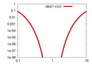
Figure 1: $\epsilon(x)$is given by the polar decomposition of order 16: $\epsilon(x)=\frac{(1+x)^{16}-(1-x)^{16}}{(1+x)^{16}+(1-x)^{16}}$.

For the overlap operator (eq.(50)) this means:

• Eq.(99) states that scaling the kernel $H_{T}$ is a valid operation.

• Eq.(100) demonstrates that the quality of the approximation to the sign function depends on this scaling. In other words, there is an optimal scaling factor.

5 Comparison of the different domain wall fermions

As demonstrated earlier, the kernels of the domain wall actions are given by (see eq.(51))

$$\mbox{M\"{o}bius:}\;(b_{i}+c_{i})\gamma_{5}D_{w}(2+(b_{i}-c_{i})D_{w})^{-1}$$ (101)

$$\mbox{Shamir:}\;a\gamma_{5}D_{w}(2+aD_{w})^{-1},$$ (102)

$$\mbox{Bori\c{c}i:}\;a\gamma_{5}D_{w},\;\;\;\mbox{Chiu:}\;a_{i}\gamma_{5}D_{w}.$$ (103)

In the following, we will show how the determination of the quark propagator depends on the choice of the coefficients $b_{i},c_{i}$ (and hence on $a,a_{i}$ as well). We will describe the advantages of the Möbius operator as compared to Shamir’s and Chiu/Boriçi’s suggestions.

5.0.1 The Möbius operator

As can be seen in eq.(101), the Möbius kernel can be scaled with the coefficient $b_{i}+c_{i}$. In other words, the eigenvalues of the operator $\gamma_{5}D_{w}(2+(b_{i}-c_{i})D_{w})^{-1}$ can be slided along the abscissa until the approximation to the sign function is optimal (with given $L_{s}$).

The coefficients $b_{i}-c_{i}$ in the denominator are different. They don’t simply act as scaling factors, but change the spectrum of the operator. In other words, for each $b_{i}-c_{i}$ one has a different matrix. Accordingly, one can use $b_{i}-c_{i}$ to tune the condition number of the kernel operator. The smaller the condition number, the better the approximation to the sign function will be.

As mentioned above, the denominator will always be chosen independent of $i$. Not so for $b_{i}+c_{i}$. We have $L_{s}$ different coefficients. This freedom allows for different choices of polynomials that approximate the sign function on the overlap side, such as the polar decomposition or Zolotarev’s polynomials (see eq.(56) and eq.(57)).

5.0.2 Shamir’s operator

Shamir’s operator allows for a tuning of the condition number, since it possesses a coefficient $a$ in the denominator. On the other hand, the same coefficient $a$ acts as the scaling factor in the numerator. Therefore this operator cannot be scaled without changing the matrix itself. In other words, in the two dimensional space, spanned by the coefficients $b_{i}+c_{i}$ and $b_{i}-c_{i}$, Shamir’s operator can only exploit the diagonal.

It follows that in this case the only possible polynomial approximation on the overlap side is Neuberger’s polar decomposition.

5.0.3 Chiu/Boriçi’s operator

Chiu/Boriçi’s action has independent coefficients $a_{i}$ that act solely as scaling factors. On the other hand, the denominator is constant (equal to 2). Therefore the condition number for Chiu/Boriçi’s operator can not be tuned. Note, that this operator correspond to the standard overlap approach, which employs Dirac fermions, with a denominator equal to the identity.

5.0.4 Conclusions

Möbius fermions are a best of two worlds approach. They combine Shamir’s tuning of the condition number with the scalability of Chiu/Boriçi’s action. Our results will demonstrate that this leads to a significant reduction of the computational costs.

6 Red/black preconditioning

The standard red/black preconditioning is only applicable for Shamir’s action. We therefore introduce a new red/black partitioning that can be employed for the Möbius operator (and hence for Shamir and Chiu/Boriçi as well).

The two preconditioning methods are defined as follows:

• Standard red/black: every neighbour of a black point is red.

• New red/black: every space-time neighbour of a black point is red, every neighbour in the fifth dimension of a black point is black.

A matrix $M$, acting on a vector $x$, can then be written as:

$$Mx=\left(\begin{array}[]{cc}M_{rr}&M_{rb}\\ M_{br}&M_{bb}\end{array}\right)\left(\begin{array}[]{c}x_{r}\\ x_{b}\end{array}\right).$$ (108)

Red/black preconditioning of this matrix is then defined through

$$LMR=\left(\begin{array}[]{cc}\hskip-4.26773ptM_{rr}&\hskip-4.26773pt0\\ \hskip-4.26773pt0&\hskip-4.26773ptM_{bb}-M_{br}M^{-1}_{rr}M_{rb}\end{array}\hskip-4.26773pt\right),$$ (111)

with

$$L\hskip-2.56064pt=\hskip-2.56064pt\left(\begin{array}[]{cc}\hskip-4.26773ptI_{rr}&\hskip-4.26773pt0\\ \hskip-4.26773pt-M_{br}M^{-1}_{rr}&\hskip-4.26773ptI_{bb}\end{array}\hskip-4.26773pt\right),R\hskip-2.84544pt=\hskip-2.84544pt\left(\begin{array}[]{cc}\hskip-4.26773ptI_{rr}&\hskip-4.26773pt-M^{-1}_{rr}M_{rb}\\ \hskip-4.26773pt0&\hskip-4.26773ptI_{bb}\end{array}\hskip-4.26773pt\right).\hskip-32.72049pt$$ (116)

$I$ is the identity operator. In principle, the two sets (red and black) can be chosen freely. But from a practical point of view, $M^{-1}_{rr}$ has be a simple matrix, since it has to be inverted in each iteration step of the linear system solver.

To keep notation simple, let’s define for the Wilson operator (eq.(9)) $\hat{m},\hat{D}$ as $D_{w}(M_{5})=\hat{m}\delta_{x,y}-1/2\hat{D}$. For standard red/black preconditioning we find

$$M^{standard}_{rr}=\hskip 76.82234pt$$ (117)

$$\left(\hskip-2.84544pt\begin{array}[]{cccc}&\cdots&&\\ -\frac{1}{2}\hat{D}^{(2)}P_{+}&b_{2}\hat{m}+1&-\frac{1}{2}\hat{D}^{(2)}P_{-}&0\\ &\cdots&&\\ &\cdots&&\\ \end{array}\hskip-2.84544pt\right).$$ (122)

This matrix is computationally too costly, due to the off diagonal terms $c_{i}\hat{D}$ (note that for Shamir’s operator $c_{i}=0$).

For the new preconditioning method, on the other hand, we find

$$M^{new}_{rr}=\hskip 76.82234pt$$ (123)

$$\left(\hskip-2.84544pt\begin{array}[]{cccc}&\hskip-2.84544pt\cdots&&\\ (c_{2}\hat{m}-1)P_{+}&\hskip-2.84544ptb_{2}\hat{m}+1&\hskip-2.84544pt(c_{2}\hat{m}-1)P_{-}&\hskip-2.84544pt0\\ &\cdots&&\\ &\cdots&&\\ \end{array}\hskip-2.84544pt\right).\hskip-31.2982pt$$ (128)

$M^{new}_{rr}$ only contains coefficients and the chiral projectors $P_{\pm}$ and thus can be inverted analytically. Therefore, its cost in the linear system solver is negligible.

The standard preconditioning, which can be applied to Shamir’s operator, results in a numerical speed up of roughly $2.6$. We find the same acceleration for the Möbius operator with the new preconditioning method. Both methods are therefore equivalent in terms of convergence, whereas only the new approach is generally applicable.

7 Results

We will present our results for the Möbius operator. As our measure of performance we count the number of Wilson Dirac applications that the linear system solver, the conjugate gradient method on the normal equation $D_{DW}^{\dagger}D_{DW}$, needs to converge (note, that even though the Möbius operator contains three Dirac matrices per row, see (eq.(1)), whereas Shamir only one, both operators only require $L_{s}$ Wilson Dirac applications per $D_{DW}$ application). The quality of the approximation to the sign function is measured via the residual mass [17, 18, 19]. We will find that Möbius’ more general set of coefficients, as compared to Shamir and Chiu/Boriçi, leads to a substantial reduction of the computational effort.

We perform our measurements on 20 quenched $16^{3}\times 32$ gauge fields, generated with the Wilson action at $\beta=6.0$.

Our point of reference will be Shamir’s operator with a widely used set of parameters, $M_{5}=1.8$ and $b_{i}-c_{i}=1.0$. We will refer to this setting as ’standard Shamir’.

For each set of parameters, we have to tune the quark mass $m$, such that the pion mass agrees with standard Shamir. Since we find the residual mass of Möbius with $L_{s}=8$ to be roughly equal to standard Shamir with $L_{s}=16$, we adjust the pion mass such that it agrees for this two cases. The pion mass dependence on the scaling factor $b_{i}+c_{i}$ is weak and will therefore be neglected.

In all graphs, the ’number of Dirac applications’ is normalized such that it represents $L_{s}$ times the number of iterations per source. Hence, we neglect a factor two, due to the normal equation, $D_{DW}^{\dagger}D_{DW}$.

Figure 2: ’Standard Shamir’ with $M_{5}=1.8$ and $b_{i}-c_{i}=1.0$

7.1 Figure 2

Fig.(2) shows the $L_{s}$ dependence of the residual mass for standard Shamir. We will compare all our results to this data.

7.2 Figure 3

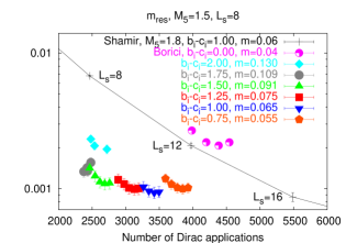
Figure 3: Comparison of the Möbius operator with standard Shamir at $m_{q}=0.06$ and $M_{5}=1.5$ (except Shamir, which uses $M_{5}=1.8$). The series of points for a given $b_{i}-c_{i}$ corresponds to different values of $b_{i}+c_{i}$. Neighbouring points represent $b_{i}+c_{i}$ values which differ by 0.1. The $b_{i}+c_{i}$ values are, $[$Boriçi: $b_{i}+c_{i}=1.0,\ldots,1.3]$, $[b_{i}-c_{i}=0.75:b_{i}+c_{i}=2.2,\ldots,2.6]$, $[b_{i}-c_{i}=1.0:b_{i}+c_{i}=2.2,\ldots,2.5]$, $[b_{i}-c_{i}=1.25:b_{i}+c_{i}=2.0,\ldots,2.4]$, , $[b_{i}-c_{i}=1.5:b_{i}+c_{i}=1.8,\ldots,2.2]$, $[b_{i}-c_{i}=1.75:b_{i}+c_{i}=1.7,\ldots,2.0]$, $[b_{i}-c_{i}=2.0:b_{i}+c_{i}=1.6,1.9,2.0]$. The optimal $b_{i}-c_{i}$ values are: Chiu/Boriçi: $b_{i}+c_{i}=1.2$, $b_{i}-c_{i}=0.75:b_{i}+c_{i}=2.5$, $b_{i}-c_{i}=1.0:b_{i}+c_{i}=2.4$, $b_{i}-c_{i}=1.25:b_{i}+c_{i}=2.3$, , $b_{i}-c_{i}=1.5:b_{i}+c_{i}=2.1$, $b_{i}-c_{i}=1.75:b_{i}+c_{i}=1.9$, $b_{i}-c_{i}=2.0:b_{i}+c_{i}=1.6$.

In fig.(3), we present our results for the Möbius operator at $L_{s}=8$ and $M_{5}=1.5$, but various $b_{i}-c_{i}$. We use a Shamir quark mass of $m=0.06$, which corresponds to a pion mass in lattice units of $m_{\pi}=0.44$. The series of points, for a given $b_{i}-c_{i}$, corresponds to different values of $b_{i}+c_{i}$. It is important to note that we choose all scaling coefficients to be the same, i.e. $b_{1}+c_{1}=b_{i}+c_{i},\;\forall\;i\;\in\;L_{s}$. In other words, we choose the polar decomposition to approximate the sign function.

In general, the number of Dirac applications increases with $b_{i}+c_{i}$. For $b_{i}+c_{i}=1.75$ this behaviour starts to change. At $b_{i}+c_{i}=2.0$ it is even reversed and the number of Dirac applications falls with growing $b_{i}+c_{i}$.

7.3 Figure 4

In fig.(4), we analyse the dependence of Möbius’ residual mass on $M_{5}$, see eq.(9). We use the optimal $b_{i}-c_{i}=1.5$, as determined in the analysis in fig.(3). Again, the number of Wilson Dirac applications increases with $b_{i}+c_{i}$. We find that the optimal $M_{5}$ values are $M_{5}=1.4$ and $M_{5}=1.5$, where $M_{5}=1.4$ reaches smaller residual masses, but $M_{5}$ requires less Wilson Dirac applications.

As can be read off from the abscissa, for the optimal $b_{i}-c_{i}$ and $M_{5}$ values, the Möbius operator is roughly two times cheaper than standard Shamir.

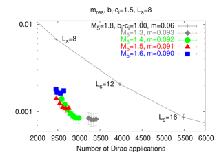
Figure 4: $M_{5}$ dependence of the Möbius operator, with optimal $b_{i}-c_{i}$ as determined in fig.(3). $M_{5}=1.4$ and $M_{5}=1.5$ are optimal, where $M_{5}=1.4$ reaches smaller residual masses, but $M_{5}$ requires less Wilson Dirac applications. The $b_{i}+c_{i}$ values are, $[M_{5}=1.3:b_{i}+c_{i}=2.9,\ldots,3.2]$, $[M_{5}=1.4:b_{i}+c_{i}=2.0,\ldots,2.6]$, $[M_{5}=1.5:b_{i}+c_{i}=1.8,\ldots,2.2]$, , $[M_{5}=1.6:b_{i}+c_{i}=1.6,\ldots,1.9]$.

7.4 Figure 5

In fig.(5), we show how Möbius’ residual mass behaves for larger $L_{s}$, with $b_{i}-c_{i}=1.5$ and $M_{5}=1.5$. Obviously, the relative improvement over standard Shamir grows rapidly.

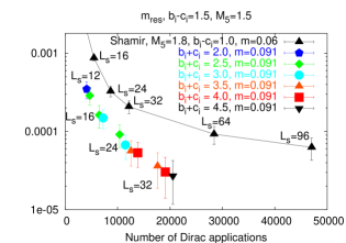
Figure 5: $L_{s}$ dependence of the residual mass, with $b_{i}-c_{i}=1.5$ and $M_{5}=1.5$. It can be seen that Möbius is numerically much better behaved than standard Shamir.

7.5 Figure 6

In fig.(6), we consider the behaviour of Möbius’ residual mass for the smaller standard Shamir quark mass $m=0.02$, with $M_{5}=1.5$ and $b_{i}-c_{i}=1.0$. Two facts are worth mentioning. Firstly, compared to the analysis with $m=0.06$, the factor of improvement for these $M_{5}$ and $b_{i}-c_{i}$ values, increases from 1.6 to 1.7. This means that the advantage of Möbius over standard Shamir grows with falling quark mass. Secondly, the optimal $b_{i}+c_{i}$ is equal to 2.4, both for $m=0.02$ and $m=0.06$. This suggest, that the tuning of the Möbius operator can be performed at heavy quark masses, where the computation of the propagators is less expensive.

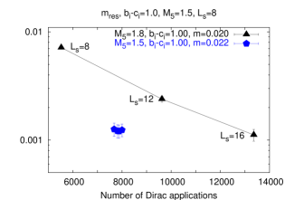
Figure 6: Residual mass, for smaller standard Shamir quark mass $m=0.02$, with $M_{5}=1.5$, $b_{i}-c_{i}=1.0$ and $b_{i}+c_{i}=2.3,\ldots,2.6$. The factor of improvement over standard Shamir grows from 1.6 to 1.7, as compare to the $m=0.06$ analysis. The optimal $b_{i}+c_{i}$ values is again 2.4, as for $m=0.06$.

7.6 Zolotarev coefficients and figure 7

As mentioned above, the scaling coefficients $b_{i}+c_{i}$ can take $L_{s}$ different values. The optimal choice for the approximation to the sign function are the Zolotarev coefficients [8]. In other words, of all possible choices for the coefficients, Zolotarev will achieve the smallest residual mass. In fig.(7) we show results that employ Zolotarev’s coefficients at $L_{s}=10$. We compare with the polar decomposition (i.e. all coefficients equal) at $L_{s}=16$. The $L_{s}$ are chosen such that the two polynomials overlap as well as possible. The graph illustrates that Zolotarev’s performance is worse than what we found for the polar decomposition. Even though Zolotarev’s $L_{s}$ is much smaller, its number of iterations in the linear system solver explodes.

This surprising behaviour is due to the fact that the convergence of the linear system solver degrades with increasing $b_{i}+c_{i}$. For Zolotarev there are always coefficients that are larger than the ones being used for the polar decomposition. Even though there are smaller ones as well, the large ones are responsible for the slow convergence.

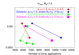
Figure 7: Comparison of Zolotarev polynomial with polar decomposition. Scale = $(b_{i}+c_{i})$ stands for a choice of the coefficients such that the Zolotarev polynomial, with $L_{s}=10$, overlaps with the polar decomposition at $L_{s}=16$ as well as possible (obviously, there is no overlap in the interval where the Zolotarev polynomial is flat).

References

• [1] H.B. Nielsen and M. Ninomiya, Nucl. Phys. B185 (1981) 20.
• [2] H.B. Nielsen and M. Ninomiya, Nucl. Phys. B193 (1981) 173.
• [3] D.B. Kaplan, Phys. Lett. B288 (1992) 342, hep-lat/9206013.
• [4] J. Callan, Curtis G. and J.A. Harvey, Nucl. Phys. B250 (1985) 427.
• [5] Y. Shamir, Nucl. Phys. B406 (1993) 90, hep-lat/9303005.
• [6] V. Furman and Y. Shamir, Nucl. Phys. B439 (1995) 54, hep-lat/9405004.
• [7] A. Borici, Nucl. Phys. Proc. Suppl. 83 (2000) 771, hep-lat/9909057.
• [8] T.W. Chiu, Phys. Rev. Lett. 90 (2003) 071601, hep-lat/0209153.
• [9] R. Narayanan and H. Neuberger, Phys. Lett. B302 (1993) 62, hep-lat/9212019.
• [10] R. Narayanan and H. Neuberger, Phys. Rev. Lett. 71 (1993) 3251, hep-lat/9308011.
• [11] R. Narayanan and H. Neuberger, Nucl. Phys. B412 (1994) 574, hep-lat/9307006.
• [12] H. Neuberger, Phys. Rev. D57 (1998) 5417, hep-lat/9710089.
• [13] H. Neuberger, Phys. Lett. B417 (1998) 141, hep-lat/9707022.
• [14] Y. Kikukawa and T. Noguchi, (1999), hep-lat/9902022.
• [15] R.G. Edwards and U.M. Heller, Phys. Rev. D63 (2001) 094505, hep-lat/0005002.
• [16] R. Brower, S. Chandrasekharan and U.J. Wiese, Phys. Rev. D60 (1999) 094502, hep-th/9704106.
• [17] Y. Aoki et al., Phys. Rev. D69 (2004) 074504, hep-lat/0211023.
• [18] CP-PACS, A. Ali Khan et al., Phys. Rev. D63 (2001) 114504, hep-lat/0007014.
• [19] T. Blum et al., Phys. Rev. D69 (2004) 074502, hep-lat/0007038.