$B_{s}$ meson excited states from the lattice

Abstract:

This is a follow-up to our earlier work [1, 2, 3] for the energies and the charge (vector) and matter (scalar) distributions for S-wave states in a heavy-light meson, where the heavy quark is static and the light quark has a mass about that of the strange quark. We now study the radial distributions of higher angular momentum states, namely P- and D-wave states. In nature the closest equivalent of this heavy-light system is the $B_{s}$ meson.

The calculation is carried out with dynamical fermions on a $16^{3}\times 32$ lattice with a lattice spacing of about 0.10 fm generated with the non-perturbatively improved clover action. It is shown that several features of the energies and radial distributions are in qualitative agreement with what one expects from a simple one-body Dirac equation interpretation.

PoS(LAT2005)205

1 Energies

The basic quantity for evaluating the energies of heavy-light mesons is the 2-point correlation function – see Fig. 1. It is defined as

$$C_{2}(T)=\langle P_{t}\Gamma G_{q}(\mathbf{x},t+T,t)P_{t+T}\Gamma^{{\dagger}}U^{Q}(\mathbf{x},t,t+T)\rangle,$$ (1)

where $U^{Q}(\mathbf{x},t,t+T)$ is the heavy (infinite mass)-quark propagator and $G_{q}(\mathbf{x},t+T,t)$ the light anti-quark propagator. $P_{t}$ is a linear combination of products of gauge links at time $t$ along paths $P$ and $\Gamma$ defines the spin structure of the operator. The $\langle...\rangle$ means the average over the whole lattice. The energies are then extracted by fitting the $C_{2}$ with a sum of exponentials,

$$C_{2}(T)\approx\sum_{i=1}^{N_{\textrm{max}}}c_{i}\mathrm{e}^{-m_{i}T}c_{i},$$ (2)

where $N_{\textrm{max}}=2$ – $4$, $T\leq 14$.

Figure 1: The two-point correlation function $C_{2}$ (on the left) and the three-point correlation function $C_{3}$ (on the right). The probe $\Theta$ is at a distance $R$ from the heavy quark.

	$\kappa$	$a$/fm	$m_{q}/m_{s}$	$r_{0}m_{\pi}$
DF3	0.1350	0.110	1.1	1.93(3)
DF4	0.1355	0.104	0.6	1.48(3)
DF5	0.1358	0.099	0.3	1.06(3)

Table 1: Lattice parameters. We use $r_{0}=0.525(25)$ fm to convert lattice results to physical units.

Calculations were made using three different lattices with $\beta=5.2$, $C_{\textrm{SW}}=2.0171$ non-perturbatively improved clover fermions. The parameters are given in Table 1 and the extracted energies are summarized in Fig. 2. The notation L$+$($-$) means that the light quark spin couples to orbital angular momentum L giving the total $j=\textrm{L}\pm 1/2$. 2S is the first radially excited L$=0$ state. Energies are given with respect to the S-wave ground state. The plot also shows a comparison between the static (infinitely heavy) and smeared (“sum6”) heavy quark. The “sum6” is APE type smearing, where the simple gauge links in the time direction are replaced by the sum of six gauge link staples. The maximum distance from the original, simple link is one lattice spacing. The effect of the smearing on energy differences seems to be small.

2 Radial distributions

For evaluating the radial distributions of the light quark a 3-point correlation function is needed – see Fig. 1. It is defined as

$$C_{3}(R,T)=\langle\Gamma^{{\dagger}}U^{Q}\Gamma G_{q1}\Theta G_{q2}\rangle.$$ (3)

We now have two light quark propagators, $G_{q1}$ and $G_{q2}$, and a probe $\Theta(R)$ at distance $R$ from the static quark. We have used two probes: $\gamma_{4}$ for the vector (charge) and $1$ for the scalar (matter) distribution. The radial distributions, $x^{ij}(R)$, are then extracted by fitting the $C_{3}$ with

$$C_{3}(R,T)\approx\sum_{i,j=1}^{N_{\textrm{max}}}c_{i}\mathrm{e}^{-m_{i}t_{1}}x^{ij}(R)\mathrm{e}^{-m_{j}t_{2}}c_{j},$$ (4)

where the $m_{i}$, $c_{i}$ are those extracted from $C_{2}$. The most recent calculations are the P$+$ and D$+-$ distributions (see Figs. 5–8). Earlier S-wave distribution calculations have been published in Refs. [1, 2].

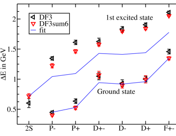
Figure 2: The energies of different angular momentum states with respect to the S-wave ground state. The error bars show the statistical error and the estimated systematic error from the extraction procedure. No continuum limit is taken. See Section 3 for more details about the Dirac model fit.

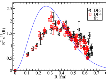
Figure 3: S-wave ground state ($x^{11}$) charge distribution.

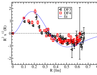
Figure 4: S-wave charge distribution: the off-diagonal correlation between the ground state and the first radially excited state. The Dirac model seems to get the node right – while no attempt has been made to fit the radial distributions.

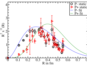
Figure 5: P-wave charge distributions.

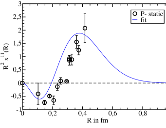
Figure 6: P-wave matter distribution. Note that the Dirac model is able to get the sign change right.

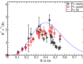
Figure 7: Comparison of static (infinitely heavy) and smeared (“sum6”) heavy quark charge distributions for the P$+$ state.

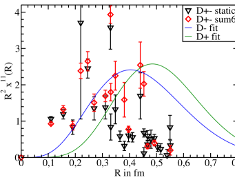
Figure 8: Comparison of static (infinitely heavy) and smeared (“sum6”) heavy quark charge distributions for the D$+-$ state.

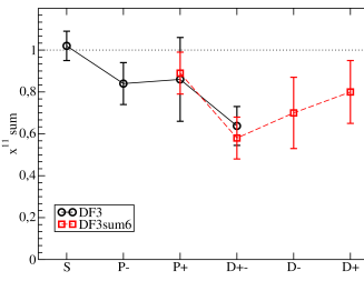
Figure 9: Charge sum rule. This should be one (the charge of the $q$) in the normalisation that is used here.

3 A model based on the Dirac equation

A simple model based on the Dirac equation is used to try to describe the lattice data. Since the mass of the heavy quark is infinite we have essentially a one-body problem. The potential in the Dirac equation has a linearly rising scalar part, $b_{\textrm{sc}}R$, as well as a vector part $b_{\textrm{vec}}R$. The OGE potential, incorporating the running coupling constant $\alpha_{s}(k^{2})$, is obtained by the replacement

$$\frac{\alpha}{R}\;\longrightarrow\;a_{\textrm{OGE}}\frac{2}{\pi}\int_{0}^{\infty}\!\!\mathrm{d}k\,j_{0}(kR)\alpha_{s}(k^{2}),\quad\alpha_{s}(k^{2})=\frac{12\pi}{27}\ln^{-1}\frac{k^{2}+4m^{2}_{g}}{\Lambda^{2}_{\textrm{QCD}}}.$$ (5)

Here $\Lambda_{\textrm{QCD}}=260$ MeV, the dynamical gluon mass $m_{g}=290$ MeV (see Ref. [4] for details) and $a_{\textrm{OGE}}$ is an overall adjustable parameter. The potential has also a scalar term $m\omega\textrm{L}(\textrm{L}+1)$ depending on the orbital angular momentum.

The solid lines in Figs. 3–8 are radial distributions from the Dirac model fit. The fit parameters are $m=0.088$ GeV, $a_{\textrm{OGE}}=0.81$, $b_{\textrm{sc}}=1.14$ GeV/fm, $b_{\textrm{vec}}=1.12$ GeV/fm and $\omega=0.028$. At present we only fit energy differences — the ground state energies and the 2S in Fig. 2 — and simply live with the resulting wavefunctions. An attempt could be made to fit the radial distributions as well.

4 Conclusions and acknowledgments

• The spin-orbit splitting is small and supports the symmetry $b_{\textrm{vec}}=b_{\textrm{sc}}$ as proposed in Ref. [5].

• There is now an abundance of lattice data to comprehend. The energies and radial distributions of S, P and D$+-$ states can be qualitatively understood by using a Dirac equation model.

J. K. and A. M. G. wish to thank the UKQCD Collaboration for providing the lattice configurations and the CSC - Scientific Computing Ltd. for providing the computer resources. J. K. and A. M. G. acknowledge support by the Academy of Finland (contract 54038), the Magnus Ehrnrooth foundation and the EU grant HPRN-CT-2002-00311 Euridice.

References

- [1] UKQCD Collaboration, A. M. Green, J. Koponen, C. Michael and P. Pennanen, Phys. Rev. D 65, 014512 (2002)
- [2] UKQCD Collaboration, A. M. Green, J. Koponen, C. Michael and P. Pennanen, Eur. Phys. J. C 28, 79 (2003)
- [3] UKQCD Collaboration, A. M. Green, J. Koponen, C. McNeile, C. Michael and G. Thompson, Phys. Rev. D 69, 094505 (2004)
- [4] T. A. Lähde, Nucl. Phys.A714, 183 (2003), hep-ph/0208110
- [5] P. R. Page, T. Goldman and J. N. Ginocchio, Phys. Rev. Lett. 86, 204 (2001), hep-ph/0002094