Scaling behavior of discretization errors in renormalization and improvement constants

Abstract

Non-perturbative results for improvement and renormalization constants needed for on-shell and off-shell $O(a)$ improvement of bilinear operators composed of Wilson fermions are presented. The calculations have been done in the quenched approximation at $\beta=6.0$, $6.2$ and $6.4$. To quantify residual discretization errors we compare our data with results from other non-perturbative calculations and with one-loop perturbation theory.

PACS numbers: 11.15.Ha and 12.38.Gc

I Introduction

In this paper we present our final results for the renormalization and improvement constants for quark bilinear operators using Wilson’s gauge action and the $O(a)$ improved Dirac action first proposed by Sheikholeslami and Wohlert Sheikholeslami and Wohlert (1985). The calculations have been done at three values of the gauge coupling, $\beta=6.0$, $6.2$, and $6.4$ in the quenched approximation. Our results represent a realization of Symanzik’s improvement program for systematically reducing discretization errors in lattice simulations Symanzik (1983a, b). Results for the improvement of the Dirac action have been obtained previously by the ALPHA collaboration and we have used these in our calculation. This paper deals with the improvement of external bilinear operators, ${\cal O}$ with ${\cal O}$ being one of the five Lorentz structures $A,V,P,S,T$.

The mixing with extra operators, both for on-shell and off-shell improvement of the operators, and the introduction of mass dependence in the renormalizaton constants has been discussed in detail in Section II of Ref. Bhattacharya et al., 2001. To summarize that discussion, and to remind the reader of the notation, the fully improved and renormalized bilinear operators at $O(a)$ are

$$(A^{R}_{I})_{\mu} \equiv Z_{A}^{0}(1+{\widetilde{b}}_{A}a{\widetilde{m}}_{ij})\big{(}A_{\mu}+ac_{A}\partial_{\mu}P-a\frac{1}{4}c^{\prime}_{A}(\overline{\psi}^{(i)}\gamma_{\mu}\gamma_{5}\overrightarrow{{\cal W}}\psi^{(j)}-\overline{\psi}^{(i)}\overleftarrow{{\cal W}}\gamma_{\mu}\gamma_{5}\psi^{(j)})\big{)}$$

$$(V^{R}_{I})_{\mu} \equiv Z_{V}^{0}(1+{\widetilde{b}}_{V}a{\widetilde{m}}_{ij})\big{(}V_{\mu}+ac_{V}\partial_{\nu}T_{\mu\nu}-a\frac{1}{4}c^{\prime}_{V}(\overline{\psi}^{(i)}\gamma_{\mu}\overrightarrow{{\cal W}}\psi^{(j)}-\overline{\psi}^{(i)}\overleftarrow{{\cal W}}\gamma_{\mu}\psi^{(j)})\big{)}$$

$$(T^{R}_{I})_{\mu\nu} \equiv Z_{T}^{0}(1+{\widetilde{b}}_{T}a{\widetilde{m}}_{ij})\big{(}T_{\mu\nu}+ac_{T}(\partial_{\mu}V_{\nu}-\partial_{\nu}V_{\mu})-a\frac{1}{4}c^{\prime}_{T}(\overline{\psi}^{(i)}i\sigma_{\mu\nu}\overrightarrow{{\cal W}}\psi^{(j)}-\overline{\psi}^{(i)}\overleftarrow{{\cal W}}i\sigma_{\mu\nu}\psi^{(j)})\big{)}$$

$$(P^{R}_{I}) \equiv Z_{P}^{0}(1+{\widetilde{b}}_{P}a{\widetilde{m}}_{ij})\big{(}P-a\frac{1}{4}c^{\prime}_{P}(\overline{\psi}^{(i)}\gamma_{5}\overrightarrow{{\cal W}}\psi^{(j)}-\overline{\psi}^{(i)}\overleftarrow{{\cal W}}\gamma_{5}\psi^{(j)})\big{)}$$

$$(S^{R}_{I}) \equiv Z_{S}^{0}(1+{\widetilde{b}}_{S}a{\widetilde{m}}_{ij})\big{(}S-a\frac{1}{4}c^{\prime}_{S}(\overline{\psi}^{(i)}\overrightarrow{{\cal W}}\psi^{(j)}-\overline{\psi}^{(i)}\overleftarrow{{\cal W}}\psi^{(j)}))\big{)}\,,$$

Here $(ij)$ (with $i\neq j$) specifies the flavor. The $Z_{\cal O}^{0}$ are renormalization constants in the chiral limit and ${\widetilde{m}}_{ij}$ is the quark mass defined in Eq. (7) using the axial Ward identity (AWI). $\overrightarrow{{\cal W}}\psi_{j}=(\overrightarrow{\mbox{$\not\!\!D$}}+m_{j})\psi_{j}+O(a^{2})$ is defined to be the full $O(a)$ improved Dirac operator for quark flavor $j$ (See Appendix in Ref. Bhattacharya et al., 2001). This ensures that the equation of motion operators give rise only to contact terms, and thus cannot change the overall normalization $Z_{\cal O}$. The normalization is chosen such that, at tree level, $c^{\prime}_{\cal O}=1$ for all Dirac structures.

We determine the improvement and renormalization constants using Ward identities. When implementing these, we have a number of choices. Two are of particular importance. First, we need to pick a discretization of the total derivatives appearing in the improvement terms proportional to $c_{A,V,T}$. Note that, because the derivatives are external to the operators, rather than internal, this choice should not impact the result for the $Z$’s or $c$’s, aside from corrections of $O(a^{2})$ which are not controlled. In fact, we will find that such higher order corrections are largely kinematical, and can be removed by the chiral extrapolations. Second, we need to choose the external states. As far as we know, there are no standard choices, and so we take either the state giving the best signal, or an average if there are several giving similar accuracy. We then use the difference of the results with those from other states as part of the estimate of the uncertainty. Although this is somewhat ad hoc, it is a well-defined procedure as long as we make consistent choices for all lattice spacings. We stress that the coefficients $\widetilde{b}_{\cal O}$ differ from the $b_{\cal O}$ used by earlier authors. These are related as

$$b_{\cal O}am_{ij}={\widetilde{b}}_{\cal O}a{\widetilde{m}}_{ij}+O(a)$$ (1)

where $m_{ij}\equiv(m_{i}+m_{j})/2$ is the average bare quark mass defined as $am_{i}=1/2\kappa_{i}-1/2\kappa_{c}$, $\kappa$ being the hopping parameter in the Sheikholeslami-Wohlert action and $\kappa_{c}$ its value in the chiral limit. At the level of $O(a)$ improvement, one has

$$\widetilde{b}_{\cal O}=(Z_{A}^{0}Z_{S}^{0}/Z_{P}^{0})b_{\cal O}\,.$$ (2)

The analogous relation between $m$ and $\widetilde{m}$ is given in Eq. (20).

In this paper we present results for those overall normalization constants, $Z^{0}_{\cal O}$, that are scale independent and the improvement constants $b_{\cal O}$, $c_{\cal O}$, and ${\widetilde{c}}_{\cal O}$. A detailed discussion of the methods has already been presented in Refs. Bhattacharya et al., 2001 and Bhattacharya et al., 1999, and we do not repeat them here. The extension of the method to full QCD has been presented in  Bhattacharya et al., 2006. Instead we concentrate on presenting the final results and new aspects of the analyses. In particular, using three lattice spacings we are able to significantly improve our understanding of residual discretization and perturbative errors by comparing our results with those obtained by the ALPHA collaboration using a non-perturbative method based on the Schrödinger functional and with the predictions of perturbation theory at one-loop order.

The remainder of this paper is organized as follows. In the next section we describe the essential features of our simulations and the types of propagator we use. Section III gives an overview of the methods we use to implement Ward identities and a summary of the results. We then run through the results from the different Ward identities that are needed to calculate $c_{A}$ (Secs. IV and V for zero and non-zero spatial momenta, respectively), $Z^{0}_{V}$ and $b_{V}$ (Sec. VI), $c_{V}$ and $\widetilde{b}_{A}-\widetilde{b}_{V}$ (Sec. VII), $Z^{0}_{A}$ (Sec. VIII), $Z^{0}_{P}/Z^{0}_{S}$ and $\widetilde{b}_{S}-\widetilde{b}_{P}$ (Sec. IX), $\widetilde{b}_{P}-\widetilde{b}_{A}$ and $\widetilde{b}_{S}$ (Sec. X), $c_{T}$ (Sec. XI), and the coefficients of the equation-of-motion operators (Sec. XII). We compare our results with those of others in Sec. XIII and with one-loop perturbation theory in Sec. XIV. We close with brief conclusions in Sec. XV.

II Details of Simulations

The parameters used in the simulations at the three values of $\beta$ are given in Table 1. The table also gives the labels used to refer to the different simulations. For the lattice scale $a$ we have taken the value determined in Ref. Guagnelli et al., 1998 using $r_{0}$ as it does not rely on the choice of the fermion action for a given $\beta$. The values of the hopping parameter $\kappa$, along with the corresponding results for the quark mass $a{\widetilde{m}}$, determined using the Axial Ward Identity (AWI), and $aM_{\pi}$ are given in Table 2 .

Label	$\beta$	$c_{SW}$	$a^{-1}$ (GeV)	Volume	$L$ (fm)	Confs.	$x_{4}$
60NPf	6.0	1.769	2.12	$16^{3}\times 48$	1.5	125	$4-18$
60NPb						112	$27-44$
62NP	6.2	1.614	2.91	$24^{3}\times 64$	1.65	70	$6-25$
						70	$39-58$
64NP	6.4	1.526	3.85	$24^{3}\times 64$	1.25	60	$8-56$

Table 1: Simulation parameters and statistics. $x_{4}$ denotes the time interval over which the chiral rotation is performed in the AWI. The initial Wuppertal source is placed at $t=0$.

Four major changes have been made in the analysis compared to our previous work Bhattacharya et al. (2001). First, the addition of the data set at $\beta=6.4$ to those at $\beta=6.0$ and $6.2$ (the latter two being unchanged from Ref. Bhattacharya et al., 2001) allows the identification of higher order contributions in the chiral extrapolations. As a result we now use quadratic or linear fits in the chiral extrapolations for all three $\beta$ values as opposed to the linear or constant fits used in Bhattacharya et al. (2001). Second, the improvement in the signal with increasing $\beta$ allows us to better determine which values of $\kappa$ to keep in the fits. We are able to use all seven values, $\kappa_{1}-\kappa_{7}$, at $\beta=6.2$ and $6.4$ whereas $\beta=6.0$ data at $\kappa=\kappa_{7}$ are too noisy (no clear plateaus in the ratios of correlators), and in some cases even the data at $\kappa=\kappa_{6}$ are too noisy to include in the fits.

The third improvement is with respect to the discretization of the derivatives in the operators. As in Refs. Bhattacharya et al., 1999, 2001, we use two discretization schemes in order to estimate the size of $O(a^{2})$ uncertainties. Most of our central values come from the “two-point scheme” (which is changed from Refs. Bhattacharya et al., 1999, 2001). This uses two-point discretization throughout the calculation, i.e. both in the axial rotation of the action, $\delta S$, and in the operators. It improves upon the scheme with the same name that we used in refs. Bhattacharya et al., 1999, 2001, in which we only used two-point discretization in the calculation of $c_{A}$ and $\delta S$, but all other operators were discretized using three-point discretization.

We estimate discretization errors using a hybrid scheme in which we use three-point discretization in all the operators but retain the two-point discretization in $\delta S$ (using the corresponding two-point values for $c_{A}$ and $\widetilde{m}$). We refer to this as the “three-point scheme”. We did not use three-point derivatives in the discretization of $\delta S$ in the present calculation for reasons of computational cost. We stress, however, that both schemes have errors starting at $O(a^{2})$. By comparing them we obtain information about about the size of these errors. Further details on the two schemes are explained later.

Lastly, we have also added the calculation of $c_{A}$ using a “four-point” discretization of derivatives which is improved to $O(a^{3})$ at the classical level. This allows us to further study discretization errors.

The fourth improvement is in the definition of the central value $x$ obtained from the jackknife fits. We now include an $O(1/N)$ correction in the single elimination jackknife procedure Hahn et al. and define

$$x={\overline{x}}+N(x_{0}-{\overline{x}})$$ (3)

where ${\overline{x}}=\sum_{N}x_{jk}/N$ is the uncorrected (and previously used) estimate, $N$ is the sample size, and $x_{0}$ is the result of the fit to the full data sample.

The reanalysis changes many of the results presented in Bhattacharya et al. (2001). The most significant changes (with final results changing by more than $1\sigma$) arise from the order and range of the fit used (for example, changing from linear to quadratic extrapolation). The other changes in the analysis lead to smaller changes in the final results. We comment below on the changes at appropriate places. Because of these changes we present here estimates from all four sets of simulations listed in Table 1, and these revised estimates supersede previously published numbers.

To highlight the improvement in the signal in various ratios of correlation functions with $\beta$, we include in Figures 10, 11, 12, 17, 20, 22, and 23 previous data from 60NP and 62NP sets for comparison. Whereas the signal is marginal at $\beta=6.0$, it improves rapidly, and by $\beta=6.4$ reliable estimates for all constants can be obtained with $O(100)$ independent configurations.

For each set of simulation parameters the quark propagators are calculated using Wuppertal smearing Gupta et al. (1991). The hopping parameter in the 3-dimensional Klein-Gordon equation used to generate the gauge-invariant smearing is set to $0.181$, which gives mean squared smearing radii of $(r/a)^{2}\approx 2.9$, $3.9$, and $5.4$ for $\beta=6.0$, $6.2$, and $6.4$ respectively.

In Table 1 we also show the time extent of the region of chiral rotation in the three-point axial Ward identities. The dependence of our results on this region was investigated at $\beta=6.0$, as shown by the two different time intervals listed under 60NPf and 60NPb. We observed no significant difference in the two results, so for our final results we average the two values weighted by their errors. In the 62NP calculation, we used two separate rotation regions with equal time extent and placed symmetrically about the source. This allowed us to average the correlation functions to improve the statistical sample. In the 64NP data set we were able to further improve the efficiency of the method by enlarging the region of insertion to include the whole lattice except for a few time slices placed symmetrically on either side of the source for the original propagator at $t=0$. This construct allows us to average the signal from forward and backward propagation with a single insertion region, (time slices $8-56$), and reduces the computational time significantly because only five inversions are required instead of the eight needed in the 60NP and 62NP studies (where forward and backward propagating correlators were calculated separately).

The five kinds of propagators we use in our calculation at $\beta=6.4$ are as follows. The initial quark propagator is calculated with a Wuppertal source on time-slice $t=0$ for all the lattices. To make explicit the construction of sources for propagators with insertions we label the two ends of the time integration region by $(t_{i},t_{f})$, which for 64NP data are $t_{i}=8$ and $t_{f}=56$ as listed in Table 1. We define the insertion operator $\delta S$ using the two-point discretization of the derivatives, whereby the discretizations for the three terms in $\delta S=2\widetilde{m}P-\partial_{4}A_{4}-ac_{A}\partial^{2}_{4}P$ are

$$\int d^{4}x\partial_{4}A_{4} \to \int d^{3}x[A_{4}(t_{f},x)-A_{4}(t_{i},x)]\,,$$

$$\int d^{4}x\partial^{2}_{4}P \to \int d^{3}x[P(t_{f}+1)-P(t_{f}-1)-P(t_{i}+1)+P(t_{i}-1)]/2\,,$$ (4)

$$\int d^{4}xP \to \int d^{3}x[P(t_{i})/2+P(t_{i}+1)+\ldots+P(t_{f}-1)+P(t_{f})/2]\,.$$

Starting with the original Wuppertal source propagator we construct the three quantities defined in Eq. 4 and use these as sources to create the propagators with insertions. The final, fifth, propagator is calculated by inserting $\gamma_{5}$ at zero 3-momentum on time slice $t=23$, $20$ and $24$ respectively for the three $\beta$ values. This is needed to study the vector Ward identity used to extract $Z_{V}$.

The quark and antiquark in the operators in $\delta S$, which have flavors we call “1” and “2” respectively, are always taken to be degenerate, i.e. $m_{1}=m_{2}$. This choice is made for computational simplicity.

III Overview of Methodology and Results

In this section we discuss technical details relevant to the implementation of all the Ward identities, and give a summary of our results.

The Ward identities can be implemented on states having any spatial momentum, and we collected data for ($0,\ 1,\ \sqrt{2},\ \sqrt{3},\ 2$) units of lattice momenta. In the extraction of $c_{A}$ we find that the results from all momenta are consistent, but only after errors proportional to $(pa)^{2}$ are taken into account. Because of these additional discretization errors, and the larger statistical errors in correlators with non-zero spatial momentum, we did not find that the results at non-zero momenta added useful information. Thus, for the calculation of all other renormalization and improvement coefficients we present results only from correlators with zero spatial momentum.

We were unable to determine the covariance matrix to sufficient accuracy to do fully correlated fits. Thus, when fitting the time dependence of correlators, or ratios of correlators, we use only the diagonal part of the covariance matrix. Similarly, fits to the quark mass dependence (which are done within the jackknife procedure) ignore correlations between the results at different masses. Also, in the analysis of the three-point axial WI identities we do not propagate the errors associated with estimates of $c_{A}$ and $c_{V}$ as we do not have a corresponding error estimate on each jackknife sample. The fully self-consistent method would be to do a simultaneous fit to all the unknown parameters, but we do not have enough statistical power to do this. Because of these shortcomings, we can make no quantitative statement about goodness of fit. Nevertheless, assuming that the fits are good, the errors in the fit parameters, which are obtained using the jackknife procedure, should be reliable.

Figure 1: Fits used to determine $\kappa_{c}$ by extrapolating 64NP results for ${\widetilde{m}}$ and $M_{\pi}^{2}$. We show quadratic fits to the two-point version of ${\widetilde{m}}$ for the two cases discussed in text (octagons label points with $c_{A}({\widetilde{m}})$ and pluses label points with chirally extrapolated $c_{A}$), and a quadratic fit to $M_{\pi}^{2}$ (diamonds).

	60NP			62NP			64NP
Label	$\kappa$	$a{\widetilde{m}}$	$aM_{\pi}$	$\kappa$	$a{\widetilde{m}}$	$aM_{\pi}$	$\kappa$	$a{\widetilde{m}}$	$aM_{\pi}$
$\kappa_{1}$	$0.1300$	$0.1442(10)$	$0.711(2)$	$0.1310$	$0.1345(6)$	$0.609(1)$	$0.1280$	$0.2106(6)$	$0.766(1)$
$\kappa_{2}$	$0.1310$	$0.1182(08)$	$0.631(2)$	$0.1321$	$0.1053(4)$	$0.522(1)$	$0.1294$	$0.1754(5)$	$0.672(1)$
$\kappa_{3}$	$0.1320$	$0.0913(06)$	$0.544(2)$	$0.1333$	$0.0728(3)$	$0.418(1)$	$0.1308$	$0.1391(4)$	$0.573(1)$
$\kappa_{4}$	$0.1326$	$0.0752(05)$	$0.488(2)$	$0.1339$	$0.0562(2)$	$0.360(2)$	$0.1324$	$0.0960(2)$	$0.449(1)$
$\kappa_{5}$	$0.1333$	$0.0561(04)$	$0.416(2)$	$0.1344$	$0.0419(2)$	$0.307(2)$	$0.1334$	$0.0682(2)$	$0.364(1)$
$\kappa_{6}$	$0.1342$	$0.0308(04)$	$0.308(3)$	$0.1348$	$0.0306(2)$	$0.261(2)$	$0.1343$	$0.0429(1)$	$0.278(2)$
$\kappa_{7}$	$0.1345$	$0.0236(35)$	$0.265(12)$	$0.1350$	$0.0248(1)$	$0.235(2)$	$0.1348$	$0.0285(1)$	$0.223(2)$
$\kappa_{c}^{(1)}$	$0.13528(2)$			$0.135854(5)$			$0.135786(3)$
$\kappa_{c}^{(2)}$	$0.13530(1)$			$0.135875(4)$			$0.135784(3)$
$\kappa_{c}^{(3)}$	$0.13539(3)$			$0.13594(2)$			$0.13578(2)$

Table 2: Values of the hopping parameter used in the various simulations, and the corresponding pseudoscalar mass $aM_{\pi}$ and quark mass $a\widetilde{m}$ defined using the $c_{A}(\widetilde{m})$ and two-point discretization (see Sec. IV). The three estimates of $\kappa_{c}$, obtained using quadratic fits, correspond to (1) the zero of $\widetilde{m}$ with mass dependent $c_{A}$, (2) the zero of $\widetilde{m}$ with chirally extrapolated $c_{A}$, and (3) the zero of $M_{\pi}^{2}$.

In Table 2 we give our results for the critical hopping parameter $\kappa_{c}$, which is needed to define the vector Ward identity (VWI) quark mass $m$. These are obtained from the fits shown in Fig. 1 (for the 64NP dataset). We fit three quantities to quadratic functions of $1/2\kappa$ (which, up to an additive shift, is the tree-level quark mass). The first quantity fit is the quark mass $\widetilde{m}$ extracted from the axial Ward identity, using a mass dependent $c_{A}(\widetilde{m})$ and two-point discretization (see Section IV below for definitions of these quantities). This is the middle curve in the plot. The second fit quantity is also $\widetilde{m}$, but now obtained using the chirally extrapolated value of $c_{A}$. This is the lower curve in the plot. Finally, the third quantity fit is $M_{\pi}^{2}$, and gives the upper curve in the plot. Only the last fit includes results for both degenerate and non-degenerate quarks, using the average value of $1/\kappa$ for the latter. As the curve shows, we find no noticeable dependence on the mass difference. The respective fit parameters are

$$a\widetilde{m}(c_{A}(\widetilde{m})) = -12.24(13)+5.57(7)\frac{1}{2\kappa}-0.610(9)\frac{1}{(2\kappa)^{2}}\,,$$

$$a\widetilde{m}(c_{A}(0)) = -15.12(11)+7.13(6)\frac{1}{2\kappa}-0.822(8)\frac{1}{(2\kappa)^{2}}\,,$$ (5)

$$a^{2}M_{\pi}^{2} = +48.3(9)-27.9(5)\frac{1}{2\kappa}+4.03(6)\frac{1}{(2\kappa)^{2}}\,.$$

From these we get three estimates of $\kappa_{c}$ which we find to be consistent; this was not the case for 60NP and 62NP data. The first estimate, $\kappa_{c}^{(1)}$, is the most direct as $\widetilde{m}$ and $c_{A}(\widetilde{m})$ are extracted together from the same two-point Ward identity (also see below), so we use it in subsequent analyses and, henceforth, drop the superscript.

If both $M_{\pi}$ and $\widetilde{m}$ are extracted from fits that include large times, where only the ground state survives, then it follows from eq. 7 below that $2\widetilde{m}\equiv M_{\pi}^{2}(2/B_{\pi}+ac_{A})+O(a^{2})$, with $B_{\pi}\propto\langle 0|P|\pi\rangle/f_{\pi}$ a quantity which is non-zero in the chiral limit (and which we will use in several places below). Thus $M_{\pi}$ and $\widetilde{m}$ should vanish at the same point. We use this fact to test the adequacy of our quadratic fits of $M_{\pi}^{2}$ versus $\widetilde{m}(c_{A}(\widetilde{m}))$ or $\widetilde{m}(c_{A}(0))$. The 64NP data, illustrated for two-point discretization of derivatives, give significant intercepts:

$$a^{2}M_{\pi}^{2} = 0.0090(23)+2.61(5)a\widetilde{m}+5.84(27)(a\widetilde{m})^{2}\quad(c_{A}(m),\beta=6.0)\,,$$

$$a^{2}M_{\pi}^{2} = 0.0098(27)+2.54(7)a\widetilde{m}+7.48(40)(a\widetilde{m})^{2}\quad(c_{A}(0),\beta=6.0)\,,$$

$$a^{2}M_{\pi}^{2} = 0.0049(13)+1.87(3)a\widetilde{m}+6.32(15)(a\widetilde{m})^{2}\quad(c_{A}(m),\beta=6.2)\,,$$

$$a^{2}M_{\pi}^{2} = 0.0043(13)+1.86(3)a\widetilde{m}+7.24(17)(a\widetilde{m})^{2}\quad(c_{A}(0),\beta=6.2)\,,$$ (6)

$$a^{2}M_{\pi}^{2} = 0.0020(12)+1.49(2)a\widetilde{m}+6.11(09)(a\widetilde{m})^{2}\quad(c_{A}(m),\beta=6.4)\,,$$

$$a^{2}M_{\pi}^{2} = 0.0059(12)+1.34(2)a\widetilde{m}+7.73(12)(a\widetilde{m})^{2}\quad(c_{A}(0),\beta=6.4)\,.$$

Using $c_{A}(\widetilde{m})$ leads to smaller intercepts, and because of this we use $a\widetilde{m}(c_{A}(\widetilde{m}))$ (rather than $a\widetilde{m}(c_{A}(0))$) when making chiral extrapolations in the subsequent analyses. We note, however, that the intercept is not small when converted into physical units ($\sim(160\ {\rm MeV})^{2}$), and does not show any significant decrease with $a$. In this context it is important to note that the range of the fits in physical units is different in the three cases and the lightest “pions” are heavy. The range of pion masses in the three cases are $550-1500$, $680-1770$ and $850-2900$ MeV respectively. Thus neglected contributions from chiral logarithms, which become significant only at lower quark masses, and higher order terms in the chiral expansion, could account for the intercept. Since the present data are well fit by a quadratic, we cannot empirically resolve the issue of what additional terms need to be included in the fits.

An important point to keep in mind is that the extrapolations to extract renormalization and improvement constants are in $a\widetilde{m}$, and are different from the usual chiral extrapolations where the control parameter is $M_{\pi}^{2}/\Lambda_{\chi}^{2}$ with $\Lambda_{\chi}\sim 1$ GeV. We do not need to be in the chiral regime for our method to work. In the ratios of correlators that appear in the Ward identities we use, the same intermediate states contribute to both numerator and denominator, and possible non-analytic behavior in the quark mass (including that from enhanced quenched chiral logarithms) cancels. What matters is that $a\widetilde{m}\ll 1$, which, as can be seen from Table 2, is reasonably well satisfied for all of our masses. Indeed, a striking feature of our results is that the quadratic fits we use work very well over our entire range of quark masses.

	60NPf	60NPb	62NP	64NP
$c_{A}$	$-0.039(08)$	$-0.037(09)$	$-0.034(03)$	$-0.032(03)$
$Z^{0}_{V}$	$+0.7689(08)$	$+0.7703(09)$	$+0.7880(04)$	$+0.8033(05)$
$\widetilde{b}_{V}$	$+1.448(20)$	$+1.413(23)$	$+1.273(10)$	$+1.212(11)$
$Z^{0}_{V}$	$+0.7689(08)$	$+0.7697(09)$	$+0.7876(03)$	$+0.8016(05)$
$b_{V}$	$+1.530(12)$	$+1.519(13)$	$+1.402(08)$	$+1.370(09)$
$Z^{0}_{V}$	$+0.773(05)*$	$+0.761(06)*$	$+0.790(02)*$	$+0.801(02)$
$\widetilde{b}_{A}-\widetilde{b}_{V}$	$-0.309(76)*$	$-0.469(77)*$	$-0.096(31)*$	$-0.123(54)$
$Z^{0}_{V}$	$+0.774(05)*$	$+0.762(06)*$	$+0.791(02)*$	$+0.800(02)$
$b_{A}-b_{V}$	$-0.288(69)*$	$-0.433(71)*$	$-0.095(29)*$	$-0.130(49)$
$Z^{0}_{V}/(Z^{0}_{A})^{2}$	$+1.203(11)*$	$+1.209(13)*$	$+1.191(06)*$	$+1.173(05)$
$\widetilde{b}_{A}-\widetilde{b}_{V}$	$-0.094(89)*$	$+0.016(96)*$	$-0.075(75)*$	$-0.131(65)$
$Z^{0}_{A}$	$+0.799(04)*$	$+0.794(05)*$	$+0.818(04)$	$+0.825(02)$
$Z^{0}_{P}/Z^{0}_{A}Z^{0}_{S}$	$+1.052(10)*$	$+1.062(12)*$	$+1.084(05)*$	$+1.089(04)$
$\widetilde{b}_{P}-\widetilde{b}_{S}$	$-0.058(65)*$	$-0.178(52)*$	$-0.096(25)*$	$-0.104(56)$
$c_{T}$	$+0.083(12)*$	$+0.088(12)*$	$+0.063(10)*$	$+0.054(05)*$
$Z^{0}_{P}/Z^{0}_{A}Z^{0}_{S}$ [$c_{A}(m)$]	$+1.051(10)*$	$+1.057(12)*$	$+1.084(05)*$	$+1.077(02)$
$\widetilde{b}_{A}-\widetilde{b}_{P}-\widetilde{b}_{m}$ [$c_{A}(m)$]	$+0.598(43)*$	$+0.629(49)*$	$+0.674(21)*$	$+0.511(09)$
$-2\widetilde{b}_{m}$ [$c_{A}(m)$]	$+1.052(72)*$	$+1.251(81)*$	$+1.313(27)*$	$+1.193(15)$
$Z^{0}_{P}/Z^{0}_{A}Z^{0}_{S}$ [$c_{A}(0)$]	$+1.055(09)*$	$+1.060(10)*$	$+1.090(05)*$	$+1.077(03)$
$\widetilde{b}_{A}-\widetilde{b}_{P}-\widetilde{b}_{m}$ [$c_{A}(0)$]	$+0.943(114)*$	$+0.932(137)*$	$+0.957(27)*$	$+0.646(28)$
$-2\widetilde{b}_{m}$ [$c_{A}(0)$]	$+1.406(107)*$	$+1.472(124)*$	$+1.428(28)*$	$+1.346(13)$

Table 3: Summary of results for the different combinations of renormalization and improvement constants extracted using the two-point derivative. The horizontal lines separate the extraction of quantities using the divergence of axial current, the conservation of charge, three-point axial chiral Ward identities, and the relation between quark masses given in Eq. 20. All unmarked estimates are based on quadratic fits in both $\widetilde{m}_{1}\equiv\widetilde{m}_{2}$ and $\widetilde{m}_{3}$. Asterisks mark values extracted using linear extrapolations in both $\widetilde{m}_{1}\equiv\widetilde{m}_{2}$ and $\widetilde{m}_{3}$. All seven masses are used at $\beta=6.2$ and $6.4$ while at $\beta=6.0$ the lightest quark ($\kappa_{7}$) is dropped. Labels $c_{A}(m)$ and $c_{A}(0)$ refer, respectively, to whether the mass dependent or chirally extrapolated value of $c_{A}$ is used in the analysis.

	60NPf	60NPb	62NP	64NP
$c_{A}$	$-0.036(16)$	$-0.038(18)$	$-0.040(05)$	$-0.035(03)$
$Z^{0}_{V}$	$+0.7677(25)$	$+0.7679(31)$	$+0.7877(04)$	$+0.8027(06)$
$\widetilde{b}_{V}$	$+1.492(68)$	$+1.499(83)$	$+1.296(10)$	$+1.233(11)$
$Z^{0}_{V}$	$+0.7672(21)$	$+0.7678(23)$	$+0.7875(03)$	$+0.8016(05)$
$b_{V}$	$+1.533(13)$	$+1.522(14)$	$+1.402(08)$	$+1.370(09)$
$Z^{0}_{V}$	$+0.771(16)@$	$+0.760(17)@$	$+0.785(03)*$	$+0.797(02)$
$\widetilde{b}_{A}-\widetilde{b}_{V}$	$-0.234(61)@$	$-0.359(57)@$	$-0.053(30)*$	$-0.174(56)$
$Z^{0}_{V}$	$+0.773(16)@$	$+0.762(17)@$	$+0.785(03)*$	$+0.797(02)$
$b_{A}-b_{V}$	$-0.210(56)@$	$-0.324(54)@$	$-0.053(29)*$	$-0.168(51)$
$Z^{0}_{V}/(Z^{0}_{A})^{2}$	$+1.198(08)@$	$+1.196(08)@$	$+1.189(05)*$	$+1.173(04)$
$\widetilde{b}_{A}-\widetilde{b}_{V}$	$-0.079(74)@$	$-0.002(83)@$	$-0.057(69)*$	$-0.009(56)$
$Z^{0}_{A}$	$+0.800(04)@$	$+0.797(04)@$	$+0.814(02)*$	$+0.824(02)$
$Z^{0}_{P}/Z^{0}_{A}Z^{0}_{S}$	$+1.051(08)@$	$+1.062(10)@$	$+1.084(05)*$	$+1.087(04)$
$\widetilde{b}_{P}-\widetilde{b}_{S}$	$+0.003(42)@$	$-0.142(36)@$	$-0.096(25)*$	$-0.033(55)$
$c_{T}$	$+0.087(11)@$	$+0.085(12)@$	$+0.071(10)*$	$+0.058(05)*$
$Z^{0}_{P}/Z^{0}_{A}Z^{0}_{S}$ [$c_{A}(m)$]	$+1.011(27)*$	$+1.009(26)*$	$+1.071(05)*$	$+1.074(03)$
$\widetilde{b}_{A}-\widetilde{b}_{P}-\widetilde{b}_{m}$ [$c_{A}(m)$]	$+0.513(110)*$	$+0.470(89)*$	$+0.617(27)*$	$+0.520(14)$
$-2\widetilde{b}_{m}$ [$c_{A}(m)$]	$+1.120(104)*$	$+1.168(92)*$	$+1.196(34)*$	$+1.183(19)$
$Z^{0}_{P}/Z^{0}_{A}Z^{0}_{S}$ [$c_{A}(0)$]	$+1.014(23)*$	$+1.010(26)*$	$+1.068(05)*$	$+1.072(03)$
$\widetilde{b}_{A}-\widetilde{b}_{P}-\widetilde{b}_{m}$ [$c_{A}(0)$]	$-0.208(253)*$	$-0.209(291)*$	$+0.187(27)*$	$+0.233(31)$
$-2\widetilde{b}_{m}$ [$c_{A}(0)$]	$+0.917(125)*$	$+0.953(135)*$	$+1.150(26)*$	$+0.918(09)$

Table 4: Summary of results for the different combinations of renormalization and improvement constants extracted using the three-point derivative. All unmarked estimates are based on quadratic fits in both $\widetilde{m}_{1}\equiv\widetilde{m}_{2}$ and $\widetilde{m}_{3}$. Asterisks mark values extracted using linear extrapolations in both $\widetilde{m}_{1}\equiv\widetilde{m}_{2}$ and $\widetilde{m}_{3}$. At $\beta=6.2$ and $6.4$, all seven masses are used. At $\beta=6.0$ the lightest quark $\kappa_{7}$ is dropped, and, for estimates marked $@$, only masses $\kappa_{1}-\kappa_{5}$ and linear fits are used. Labels $c_{A}(m)$ and $c_{A}(0)$ refer, respectively, to whether the mass dependent or chirally extrapolated value of $c_{A}$ is used in the analysis.

64NP
	2pt		3pt
	$c_{A}(m)$	$c_{A}(0)$	$c_{A}(m)$	$c_{A}(0)$
extrapolation	$-0.167(90)$	$-0.136(90)$	$-0.042(71)$	$-0.092(69)$
$1/m$ fit	$-0.079(07)$	$-0.090(08)$	$-0.099(08)$	$-0.079(06)$
slope ratio	$-0.088(10)$	$-0.085(10)$	$-0.066(08)$	$-0.074(08)$
62NP
	2pt		3pt
	$c_{A}(m)$	$c_{A}(0)$	$c_{A}(m)$	$c_{A}(0)$
extrapolation	$-0.143(166)$	$-0.128(164)$	$+0.008(160)$	$-0.036(157)$
$1/m$ fit	$-0.104(17)$	$-0.124(20)$	$-0.161(20)$	$-0.120(19)$
slope ratio	$-0.116(23)$	$-0.117(23)$	$-0.103(21)$	$-0.105(21)$
60NPf
	2pt		3pt
	$c_{A}(m)$	$c_{A}(0)$	$c_{A}(m)$	$c_{A}(0)$
extrapolation	$-0.058(157)$	$-0.075(170)$	$+0.158(115)$	$-0.015(188)$
$1/m$ fit	$-0.138(25)$	$-0.189(47)$	$-0.230(43)$	$-0.143(58)$
slope ratio	$-0.136(23)$	$-0.143(28)$	$-0.092(16)$	$-0.102(16)$
60NPb
	2pt		3pt
	$c_{A}(m)$	$c_{A}(0)$	$c_{A}(m)$	$c_{A}(0)$
extrapolation	$+0.068(162)$	$+0.112(186)$	$-0.087(156)$	$-0.036(211)$
$1/m$ fit	$-0.132(23)$	$-0.176(44)$	$-0.221(43)$	$-0.139(60)$
slope ratio	$-0.123(27)$	$-0.128(35)$	$-0.089(25)$	$-0.104(26)$

Table 5: Results for $c_{V}$ using the two-point discretization data. See text (sec. VII) and Ref. Bhattacharya et al. (2001) for details. The labels $c_{A}(m)$ and $c_{A}(0)$ refer to whether the mass-dependent or chirally extrapolated value of $c_{A}$ was used in the analysis.

With $a\widetilde{m}$ and $\kappa_{c}$ in hand we carry out the analysis for two-point and three-point Ward identities discussed in Ref. Bhattacharya et al., 2001. Each identity allows us to extract one or more combinations of on-shell improvement and normalization constants. Since many of the results for 60NP and 62NP data sets given in Bhattacharya et al. (2001) have changed as a result of our reanalysis, estimates from all three lattice spacings are given in Tables 3 and 4. Similarly, a detailed comparison of the results for $c_{V}$ obtained using the methods discussed in Ref. Bhattacharya et al., 2001 is given in Table 5 for all three values of $\beta$.

Our final results for the individual constants are collected in Table 6. We quote both a statistical error (given by the single elimination jackknife procedure, in which we repeat the entire analysis on each jackknife sample), and an estimate of the residual $O(a)$ uncertainty. The latter is taken to be the difference in results obtained using two- and three-point discretizations of the derivatives except for $b_{V}$ where there is no three-point estimate. A different estimate of the uncertainties can be obtained by comparing our results to previous estimates by the ALPHA collaboration Lüscher et al. (1997a, b); Guagnelli and Sommer (1998) summarized in Table 6, by the QCDSF collaboration given in Table 9 Bakeyev et al. (2004) and by the SPQcdR collaboration Becirevic et al. (2004).

	$\beta=6.0$			$\beta=6.2$			$\beta=6.4$
	LANL	ALPHA	P. Th.	LANL	ALPHA	P. Th.	LANL	ALPHA	P. Th.
$c_{SW}$	1.769	1.769	1.521	1.614	1.614	1.481	1.526	1.526	1.449
$Z^{0}_{V}$	$+0.7695(8)(19)$	$+0.7809(6)$	$+0.810$	$+0.7878(4)(2)$	$+0.7922(4)(9)$	$+0.821$	$+0.8024(5)(2)$	$+0.8032(6)(12)$	$+0.830$
$Z^{0}_{A}$	$+0.797(4)(2)$	$+0.7906(94)$	$+0.829$	$+0.815(2)(1)$	$+0.807(8)(2)$	$+0.839$	$+0.825(2)(1)$	$+0.827(8)(1)$	$+0.847$
$Z^{0}_{P}/Z^{0}_{S}$	$+0.840(7)(15)$	$+0.840(8)$	$+0.956$	$+0.883(4)(6)$	$+0.886(9)$	$+0.959$	$+0.894(3)(4)$	$+0.908(9)$	$+0.962$
$c_{A}$	$-0.036(8)(3)$	$-0.083(5)$	$-0.013$	$-0.034(3)(6)$	$-0.038(4)$	$-0.012$	$-0.032(3)(3)$	$-0.025(2)$	$-0.011$
$c_{V}$	$-0.13(2)(3)$	$-0.32(7)$	$-0.028$	$-0.12(2)(2)$	$-0.21(7)$	$-0.026$	$-0.09(1)(2)$	$-0.13(5)$	$-0.024$
$c_{T}$	$+0.085(12)(1)$	N.A.	$+0.020$	$+0.063(10)(8)$	N.A.	$+0.019$	$+0.054(5)(4)$	N.A.	$+0.018$
$\widetilde{b}_{V}$	$+1.43(2)(7)$	N.A.	$+1.106$	$+1.27(1)(2)$	N.A.	$+1.099$	$+1.21(1)(2)$	N.A.	$+1.093$
$b_{V}$	$+1.52(1)$	$+1.48(2)$	$+1.274$	$+1.40(1)$	$+1.41(2)$	$+1.255$	$+1.37(1)$	$+1.36(3)$	$+1.239$
$\widetilde{b}_{A}-\widetilde{b}_{V}$	$-0.21(6)(5)$	N.A.	$-0.002$	$-0.09(4)(2)$	N.A.	$-0.002$	$-0.13(5)(6)$	N.A.	$-0.002$
$b_{A}-b_{V}$	$-0.36(7)(13)$	N.A.	$-0.002$	$-0.10(3)(8)$	N.A.	$-0.002$	$-0.13(5)(3)$	N.A.	$-0.002$
$\widetilde{b}_{P}-\widetilde{b}_{S}$	$-0.12(6)(5)$	N.A.	$-0.066$	$-0.10(3)(1)$	N.A.	$-0.062$	$-0.10(6)(7)$	N.A.	$-0.059$
$\widetilde{b}_{A}-\widetilde{b}_{P}+\widetilde{b}_{S}/2$	$+0.61(5)(12)$	N.A.	$+0.585$	$+0.67(2)(6)$	N.A.	$+0.579$	$+0.51(1)(1)$	N.A.	$+0.575$
$\widetilde{b}_{S}$	$+1.15(8)(1)$	N.A.	$+1.172$	$+1.31(3)(12)$	N.A.	$+1.161$	$+1.19(2)(1)$	N.A.	$+1.151$
$\widetilde{b}_{A}$	$+1.22(6)(11)$	N.A.	$+1.104$	$+1.19(4)(5)$	N.A.	$+1.097$	$+1.09(5)(6)$	N.A.	$+1.092$
$b_{A}$	$+1.16(7)(10)$	N.A.	$+1.271$	$+1.31(3)(4)$	N.A.	$+1.252$	$+1.24(5)(4)$	N.A.	$+1.237$
$\widetilde{b}_{P}$	$+1.02(9)(15)$	N.A.	$+1.105$	$+1.19(4)(3)$	N.A.	$+1.099$	$+1.13(6)(1)$	N.A.	$+1.093$

Table 6: Final results for improvement and renormalization constants. The first error in LANL estimates (this work) is statistical, and the second, where present, corresponds to the difference between using 2-point and 3-point discretization of the derivative. We quote both ${\widetilde{b}}_{V},{\widetilde{b}}_{A}$ and $b_{V},b_{A}$ to simplify comparison with previous results. Estimates for $Z_{P}^{0}/Z_{S}^{0}$ by the ALPHA collaboration are taken from Ref. Becirevic et al. (2004) and the rest from Refs. Lüscher et al. (1997a, b); Guagnelli and Sommer (1998). The final column gives the results from one-loop tadpole improved perturbation theory Ref. Bhattacharya et al. (2001).

We collect separately, in Table 7, our results for the improvement constants $c_{X}^{\prime}$, the coefficients of the equation-of-motion operators. These are discussed in Sec. XII. In sections XIII and XIV we present an analysis of residual discretization errors by comparing our estimates with those by the ALPHA collaboration and with one-loop tadpole improved perturbation theory estimates summarized in Table 6.

	60NPf	60NPb	62NP	64NP
$c^{\prime}_{V}+c^{\prime}_{P}$	$2.97(26)$	$2.66(36)$	$+2.68(9)$	$2.51(13)$
$c^{\prime}_{A}+c^{\prime}_{P}$	$2.56(20)$	$2.54(24)$	$+2.44(10)$	$2.23(12)$
$2c^{\prime}_{P}$	$2.98(41)$	$2.76(43)$	$+2.99(13)$	$2.12(22)$
$c^{\prime}_{S}+c^{\prime}_{P}$	$2.54(14)$	$2.54(15)$	$+2.38(7)$	$2.36(11)$
$c^{\prime}_{T}+c^{\prime}_{P}$	$2.58(19)$	$2.48(23)$	$+2.45(11)$	$2.40(13)$
$c^{\prime}_{V}$	$1.48(31)$	$1.28(32)$	$+1.19(10)$	$1.45(13)$
$c^{\prime}_{A}$	$1.07(27)$	$1.16(24)$	$+0.94(11)$	$1.17(11)$
$c^{\prime}_{P}$	$1.49(21)$	$1.38(22)$	$+1.50(7)$	$1.06(11)$
$c^{\prime}_{S}$	$1.05(22)$	$1.16(19)$	$+0.89(9)$	$1.30(10)$
$c^{\prime}_{T}$	$1.09(25)$	$1.10(22)$	$+0.95(12)$	$1.34(12)$

Table 7: Results for off-shell mixing coefficients using the two-point derivative data and $c_{A}(\widetilde{m})$.

IV Calculation of $c_{A}$

The calculation of $c_{A}$ exploits the two-point axial Ward identity

$$\frac{\sum_{\vec{x}}\langle\partial_{\mu}[A_{\mu}+ac_{A}\partial_{\mu}P]^{(ij)}(\vec{x},t)J^{(ji)}(0)\rangle}{\sum_{\vec{x}}\langle P^{(ij)}(\vec{x},t)J^{(ji)}(0)\rangle}=2{\widetilde{m}}_{ij}+O(a^{2})\,,$$ (7)

which also defines the quark mass ${\widetilde{m}}_{ij}$. Here the superscript $(ij)$ refer to the mass (flavor) labels ($\kappa_{i}\kappa_{j}$) of the quark and the antiquark. Up to corrections of $O(a^{2})$, this ratio of correlators should be independent of the source $J$ and the time $t$ provided $c_{SW}$ (the coefficient of the Sheikholeslami-Wohlert term in the action) and $c_{A}$ are tuned to their non-perturbative values. Since this criterion is automatically satisfied when the correlators are saturated by a single state, the determination of $c_{A}$ relies on the contribution of excited states at small $t$.

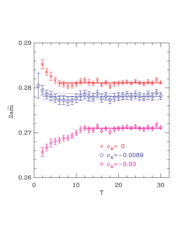
Figure 2: Estimates of $2a{\widetilde{m}}_{ij}$ for different values of $c_{A}$ illustrated using $i=j=\kappa_{3}$, $J=P$, and two-point discretization in the 64NP data set. For this quark mass, $c_{A}=-0.0089$ extends the plateau to the earliest allowed time slice $t=2$. To show sensitivity to the tuning we contrast this best fit with those using $c_{A}=0$ and $c_{A}=-0.03$, the latter being close to the chirally extrapolated value.

The sensitivity of the ratio (7) to $c_{A}$ is illustrated for the 64NP data in Fig 2. We find that, for $J=P$, the contribution of higher excited states is significant only at time-slices $t=1-5$ for all three values of $\beta$ (see Bhattacharya et al. (2001) for data at $\beta=6.0$ and $6.2$). For two-point and four-point discretization, the data at $t=1$ cannot be used to extract $c_{A}$ as the discretization of $\partial_{4}^{2}P(t=1)$ in Eq. 7 overlaps with the source at time slice $t=0$. Consequently, only the range $2\leq t\leq 5$ is sensitive to tuning $c_{A}$ and we choose $c_{A}$ to make $\widetilde{m}_{ij}$ as flat as possible for timeslices $t\geq 2$. This is done by minimizing the $\chi^{2}$ for a fit to a constant, as illustrated in Fig. 2. For three-point discretization we can implement the same choice only for $t\geq 3$. The $J=A_{4}$ data are not presented as they are dominated by the ground state already at $t\leq 4$ and are thus not sensitive to the choice of $c_{A}$. Results for $\widetilde{m}$ with different choices of discretization are collected in Table 8.

	60NP			62NP			64NP
Label	2-pt	3-pt	4-pt	2-pt	3-pt	4-pt	2-pt	3-pt	4-pt
$(\kappa_{1},\kappa_{1})$	$0.1442(10)$	$0.1425(13)$	$0.1450(10)$	$0.1345(6)$	$0.1340(7)$	$0.1349(6)$	$0.2106(6)$	$0.2108(9)$	$0.2110(6)$
$(\kappa_{2},\kappa_{2})$	$0.1182(8)$	$0.1167(11)$	$0.1188(8)$	$0.1053(4)$	$0.1048(5)$	$0.1058(4)$	$0.1754(5)$	$0.1752(7)$	$0.1756(5)$
$(\kappa_{3},\kappa_{3})$	$0.0913(6)$	$0.0902(8)$	$0.0920(6)$	$0.0728(3)$	$0.0722(3)$	$0.0727(3)$	$0.1391(4)$	$0.1389(5)$	$0.1394(4)$
$(\kappa_{4},\kappa_{4})$	$0.0752(5)$	$0.0744(7)$	$0.0757(5)$	$0.0562(2)$	$0.0558(3)$	$0.0561(2)$	$0.0960(2)$	$0.0958(3)$	$0.0963(2)$
$(\kappa_{5},\kappa_{5})$	$0.0561(4)$	$0.0555(6)$	$0.0563(4)$	$0.0419(2)$	$0.0417(2)$	$0.0421(2)$	$0.0682(2)$	$0.0681(2)$	$0.0686(2)$
$(\kappa_{6},\kappa_{6})$	$0.0308(4)$	$0.0312(15)$	$0.0310(4)$	$0.0306(2)$	$0.0304(2)$	$0.0307(2)$	$0.0429(1)$	$0.0428(1)$	$0.0430(1)$
$(\kappa_{7},\kappa_{7})$	$0.0236(35)$	$0.0251(55)$	$0.0246(30)$	$0.0248(1)$	$0.0247(2)$	$0.0250(1)$	$0.0285(1)$	$0.0284(1)$	$0.0286(1)$

Table 8: Values of the quark mass $a\widetilde{m}$ defined using the mass-dependent $c_{A}$ for two-point, three-point and four-point discretization schemes at the three couplings.

As noted in Ref. Collins et al. (2003), a possible problem with our criterion for determining $c_{A}$ is that it does not involve the same physical distances at all couplings. The “physical” criterion we wish to implement is that the same value of $\widetilde{m}_{ij}$ is obtained in the AWI from both the ground and the first excited states. This requires that we tune the source to produce the same mixture of ground and excited states at all values of $a$. While the lattice size and the radius of the smeared source in the generation of quark propagators were increased with $\beta$, they were not tuned. In fact, we find that our fit is sensitive to the same range, $t=2-5$ ($3-5$ for three-point discretization), for all three lattice spacings, and thus is sensitive to significantly shorter Euclidean times at $\beta=6.4$ than at $\beta=6$.

The part of our analysis which is, therefore, sensitive to the extent to which our criterion is physical is the manner in which the continuum limit is approached. With a physical criterion, the dominant correction to scaling will be proportional to $a^{2}$. If one changes the criterion as $a$ is varied, the simple power dependence can be distorted. While the data suggests that the contribution from higher states is small, we cannot rule out some distortion and the scaling analysis has to be taken with caution. To study the question in detail, however, would require a more extensive data set than ours.

In Figs 3, 4 and 5 we show quadratic fits to $c_{A}(\widetilde{m})$ versus $\widetilde{m}$ for the two-point, three-point and four-point discretization of the derivative. The data are for zero momentum correlators at $\beta=6.0$, $6.2$ and $6.4$, and include degenerate and non-degenerate mass combinations. The results for two-point and three-point discretizations are given in Tables 3 and 4. The four-point estimates are $0.034(8)$, $0.034(9)$, $0.030(4)$ and $0.030(3)$ for 60NPf, 60NPb, 62NP and 64NP data sets respectively. We find that the three estimates agree within errors in the chiral limit. By contrast, the $O(am)$ contributions are significant, as shown by the large, roughly linear, dependence of $c_{A}$ on $\widetilde{m}$. However, as we now explain, the bulk of this linear dependence has a simple kinematic origin and can be understood analytically.

In Ref. Bhattacharya et al. (2001) we showed that if, by tuning $c_{A}$ and $\widetilde{m}$, eq. (7) can be satisfied over a common range of time-slices where two- and three-point discretizations schemes are implemented then, to $O(a^{3})$, $\widetilde{m}$ is the same in both schemes and the $c_{A}$ at any $a\widetilde{m}$ are related as $c_{A}^{3-pt}=c_{A}^{2-pt}-{\widetilde{m}}a/2+O(a^{2})$. It is useful to generalize this argument to provide the relation between $c_{A}$ determined in any two discretization schemes. The equation we wish to satisfy is $\partial_{4}A_{4}+ac_{A}\partial^{2}_{4}P-2{\widetilde{m}}P=0$. Taylor expansion of any lattice version of this relation using a symmetric discretization scheme for the derivatives gives

$$[\partial_{4}A_{4}+a^{2}\alpha\partial^{3}_{4}A_{4}+O(a^{4})]+ac_{A}[\partial_{4}^{2}P+a^{2}\beta\partial^{4}_{4}P+O(a^{4})]-2{\widetilde{m}}[P+a^{2}\gamma\partial^{2}_{4}P+O(a^{4})]=0\,.$$ (8)

The key assumption is that this relation can be satisfied by two discretization schemes over a common range of timeslices. If so, then it follows, first, that the two schemes will give the same $\widetilde{m}$ to $O(a^{3})$ and, second, that

$$c_{A}^{(2)}-c_{A}^{(1)}=2a\widetilde{m}(\alpha^{(1)}-\alpha^{(2)}-\gamma^{(1)}+\gamma^{(2)})+O(a^{2})\,.$$ (9)

For the two-point and three-point derivatives we have used, this condition reduces to $c_{A}^{3-pt}=c_{A}^{2-pt}-a\widetilde{m}/2+O(a^{2})$ because $\alpha^{2-pt}=1/24$, $\gamma^{2-pt}=1/8$, $\alpha^{3-pt}=1/6$, and $\gamma^{3-pt}=0$. Our data confirm these two predictions to good accuracy: the ratio of correlators ($2\widetilde{m}_{ij}$) is the same within errors for the three discretization schemes, as shown in Table 8, and Eq. 9 holds, as illustrated in Figs. 3, 4 and 5 where we also plot the quantity $c_{A}^{3-pt}-c_{A}^{2-pt}+a\widetilde{m}/2$ and show it is consistent with zero at the 1-$\sigma$ level.

The UKQCD collaboration Collins et al. (2003) has pointed out that the mass dependence of $c_{A}$ can be reduced using higher order discretization schemes. This also follows from Eq. 9. For any $O(a^{3})$ improved scheme, $\alpha=\gamma=0$, and consequently $c_{A}^{imp}=c_{A}^{2-pt}-a{\widetilde{m}}/6+O(a^{2})$. In fact we find that the slope of $c_{A}^{2-pt}$ versus $a\widetilde{m}_{ij}$ is $\Delta\approx 0.18$, $0.18$ and $0.19$ respectively for $\beta=6$, $6.2$ and $6.4$, so that the slope obtained using any $O(a^{3})$ improved scheme should indeed be very small, $\Delta-1/6\sim 0.02$. For our four-point discretization scheme (which is $O(a^{3})$ improved, but differs from the five-point scheme used in Ref. Collins et al., 2003) we find that the slope is $\leq 0.03$ for all four data sets as shown in Figs 3, 4 and 5. We also find that the contribution of the $(a\widetilde{m})^{2}$ term in the four-point scheme is comparable to the linear term over the range of quark masses simulated, and to the errors. Because of the size of these higher order terms, further improvements in the discretization of the derivative are not expected to reduce the undertainty.

We stress that we do not expect a higher order scheme to completely remove $a\widetilde{m}$ contributions in $c_{A}$, for to do so would require complete implementation of an $O(a^{2})$ improvement program. Nevertheless, our results indicate that the bulk of the slope for two- and three-point discretization is due to errors associated with discretization of the derivative.

The upshot of this discussion is as follows. On the one hand, it would have been advantageous to use a higher-order discretization scheme with a smaller slope $\Delta$. This would have reduced the uncertainty in the results for some of the $b_{\cal O}$ that are proportional to $\Delta$, as discussed in later sections. On the other hand the $O(a\widetilde{m})^{2}$ and $O(a\widetilde{m})$ terms become comparable in our four-point data, and the error in the extrapolated value does not decrease compared to the lower-order schemes. Having demonstrated that the dominant effect is kinematic, we can remove it in our two- and three-point schemes simply by using the mass-dependent $c_{A}(\widetilde{m})$ in the improved axial current, rather than $c_{A}(0)$. This is indeed what we do in the axial rotation $\delta S$ (which, we recall, is always defined with two-point derivatives and in which we always use the two-point $c_{A}(\widetilde{m})$).

We now return to the numerical results for $c_{A}(0)$, which are given in Tables 3 and 4. Results from two-, three- and four-point discretizations should differ only by terms of relative size $a\Lambda_{QCD}$. In fact, as already noted, Figs 3, 4 and 5 show that the quadratically extrapolated values for $c_{A}$ at each of the three $\beta$ from all three discretization schemes agree. Estimates using linear fits, however, differ by combined $1\sigma$ errors, due to the curvature.

In Ref. Bhattacharya et al., 2001 we chose, for our central value, $c_{A}$ from the two-point discretization of the derivative over that from the three-point derivative for the following two reasons. First, the $O(a^{2})$ discretization errors in the derivatives are smaller, which leads to a smaller slope of $c_{A}$ versus $\widetilde{m}$; and second, because the statistical errors are smaller. Now that we understand the relative size of the slope to be largely a kinematical effect, and the extrapolated values overlap, and the uncertainty in the estimates are comparable, we take the weighted mean of the two-, three- and four-point results for our central value at all three lattice spacings. In addition to statistical errors we quote the spread of the results to estimate the residual $O(a)$ errors. Note that, as pointed out in the Introduction, the choice of the discretization scheme used for the derivative does not affect results for $c_{A}(0)$ at the leading order of overall improvement, and the estimates from any scheme can be used to define the improved theory. However, if a calculation requires the axial vector Ward identity be respected, then the appropriate discretization scheme and the corresponding $c_{A}(m)$ should be used.

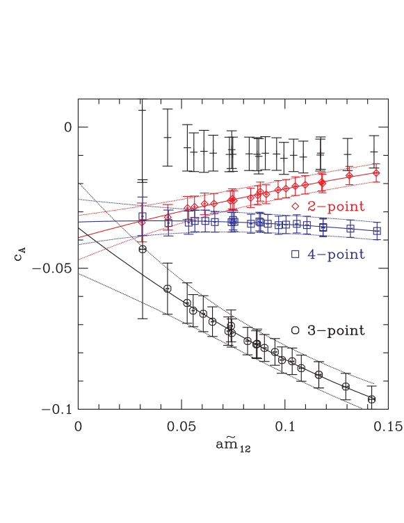
Figure 3: Results of chiral extrapolation of $c_{A}$ data at $\beta=6.0$ (60NPf) for the two-point, three-point and four-point discretization of the derivative. Quadratic fits are made to all degenerate and non-degenerate mass combinations using $\kappa_{1}-\kappa_{7}$. We also show the quantity $c_{A}^{3-pt}-c_{A}^{2-pt}+a\widetilde{m}/2$ discussed in the text using the symbol plus.

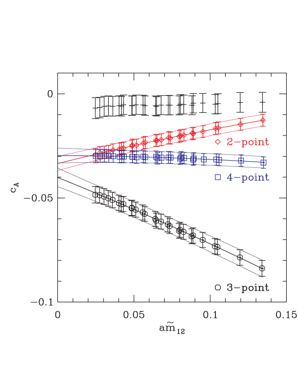
Figure 4: Same as Fig. 3 but at $\beta=6.2$.

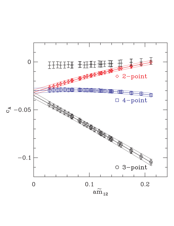
Figure 5: Same as Fig. 3 but at $\beta=6.4$.

V Extracting $c_{A}$ using states at finite momentum

The data at $\beta=6.2$ and $6.4$ are precise enough to extract $c_{A}$ using states having non-zero momenta. In figures 6 and 7 we show the results of linear fits for the chirally extrapolated value of $c_{A}$ for two-, three-, and four-point discretization of the derivative as a function of $(pa)^{2}$. For the chiral extrapolation of $c_{A}(\widetilde{m})$, quadratic fits to all mass combinations of $\kappa_{1}-\kappa_{7}$ propagators work very well at all five values of $pa$. The signal in three-point data at $pa=2$ is noisy and this is reflected in the errors. The data exhibit the following two features:

• Additional discretization errors of $O(p^{2}a^{2})$ are generated when using states with non-zero momenta. The coefficients of these corrections are significant, lying in the range $0.12-0.22$.

• The difference in results between the two-, three- and four-point discretization of the derivative decreases significantly between $\beta=6.2$ and $6.4$.

Overall, the consistency of the estimates between the two-, three- and four-point discretization schemes, the added information from fits versus $(pa)^{2}$, and the expected improvement with $\beta$ enhance our confidence in our quoted estimate of $c_{A}$.

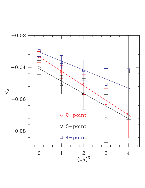
Figure 6: $c_{A}$ using states of non-zero momentum plotted against $(pa)^{2}$, along with a linear fit. We show results for the two-point, three-point and four-point discretization of the derivative. The data are for $\beta=6.2$ and $pa$ is in units of $2\pi/24$.

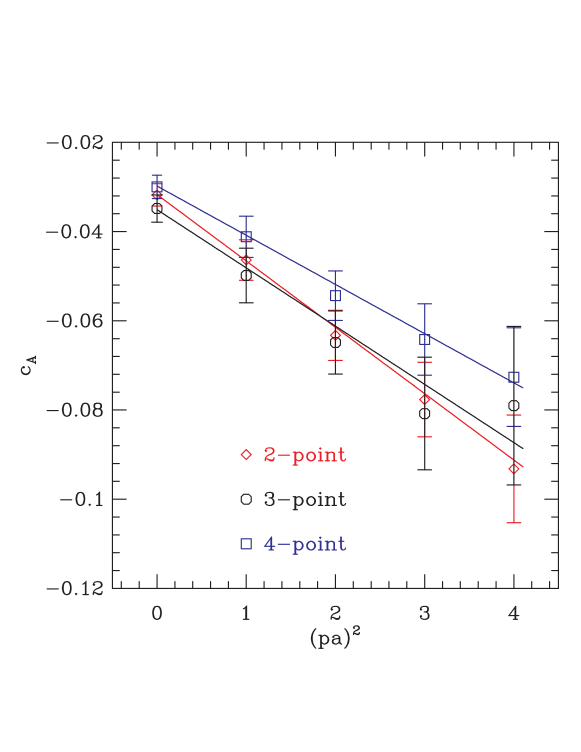
Figure 7: $c_{A}$ using states of non-zero momentum at $\beta=6.4$. Notation as in Fig. 6.

VI $Z_{V}^{0}$ and $b_{V}$

Our best estimate of $Z_{V}^{0}$ comes from the matrix elements of the vector charge $\int d^{3}xV_{4}^{(23)}(x)$ between pseudoscalar mesons

$$\frac{1}{Z_{V}^{0}(1+\widetilde{b}_{V}a\widetilde{m}_{2})} = \frac{\sum_{\vec{x},\vec{y}}\langle P^{(12)}(\vec{x},\tau)(V_{I})_{4}^{(23)}(\vec{y},t)J^{(31)}(0)\rangle}{\langle\sum_{\vec{x}}P^{(12)}(\vec{x},\tau)J^{(21)}(0)\rangle}\,.$$ (10)

with $\tau>t>0$ and the superscript $(23)$ denoting the flavor of the two fermions in the bilinear (which are taken to be degenerate). Our results for this ratio, illustrated by those in Fig. 8, show two features of particular interest: first, there is a significant dependence on $t$ for time slices close to the source or sink; and, second, there is a clear difference between the results using $J=P$ and $J=A_{4}$. Both features are indicative of $O(a^{2})$ corrections, since, aside from such corrections the ratio should be independent both of $t$ and the choice of source. The observed effect is $(1-5)\ a^{2}\Lambda_{QCD}^{2}$ using $\Lambda_{QCD}=300\;$MeV. Since neither feature would be present if the source and the sink coupled to a single state (irrespective of improvement), our results show that the separation between source and sink in our calculation is insufficient to isolate the lowest state for any value of $t$. We stress, however, that this is not a problem for implementing the improvement program (since, after all, we expect ambiguities of $O(a^{2})$).

To obtain our central values we average the $J=P$ and $J=A_{4}$ data within the jackknife procedure as they are of similar quality. There is a slight difference in results for $Z_{V}^{0}$ using two- and three-point derivatives, as shown in Tables 3 and 4. Also, at $\beta=6.0$, the errors in the three-point estimates are almost three times as large. These differences arise during the chiral extrapolation because the $\widetilde{m}$ and $\kappa_{c}$ are slightly different for the two cases and the errors in $c_{A}(\widetilde{m})$ are $2-3$ times larger for the three-point data. The difference between linear and quadratic chiral extrapolation, as shown in Fig. 9, is significant. For our central values we use quadratic extrapolations of the two-point data.

To extract $Z_{V}$, ${\widetilde{b}}_{V}$ and ${b}_{V}$ we fit the ratio in eq. (10) to a quadratic function of both $\widetilde{m}$ and the VWI mass. At $\beta=6.4$ the fits yield

$$Z_{V} = 0.8033(5)\left[1+1.212(11){\widetilde{m}}a+1.134(39)({\widetilde{m}}a)^{2}\right]\,,$$ (11)

$$Z_{V} = 0.8016(5)\left[1+1.370(9)ma+0.033(24)(ma)^{2}\right]\,.$$ (12)

The two intercepts, which give $Z_{V}^{0}$, differ by 3-$\sigma$ at $\beta=6.4$ and by $\leq 1$-$\sigma$ at $\beta=6.0$ and $6.2$. For the final estimate of $Z_{V}^{0}$ we choose the weighted average as they are of similar quality. The coefficient of the linear term in the two fits gives ${\widetilde{b}}_{V}$ and ${b}_{V}$ respectively.

In Table 9 we compare results with those from other non-perturbative calculations that have been done with the same $O(a)$ improved fermion action but utilizing different initial and final states to measure the charge. We find that the results for $b_{V}$ agree within the combined $1\sigma$ uncertainties and the expected differences of $O(a)$. For $Z_{V}^{0}$, there is a significant difference between the LANL and the ALPHA Lüscher et al. (1997a, b); Guagnelli and Sommer (1998) collaboration values, which we show, in section XIII, can be explained as residual $O(a^{2})$ effects. Estimates by the QCDSF Bakeyev et al. (2004) and the SPQcdR Becirevic et al. (2004) collaboration lie in the range defined by the LANL and ALPHA data.

	$\beta=6.0$			$\beta=6.2$			$\beta=6.4$
	LANL	ALPHA	QCDSF	LANL	ALPHA	QCDSF	LANL	ALPHA	QCDSF
$Z^{0}_{V}$	$0.7695(8)$	$0.7809(6)$	$0.7799(7)$	$0.7878(4)$	$0.7922(4)(9)$	$0.7907(3)$	$0.8024(5)$	$0.8032(6)(12)$	$0.8027(2)$
$b_{V}$	$1.52(1)$	$1.48(2)$	$1.497(13)$	$1.40(1)$	$1.41(2)$	$1.436(8)$	$1.37(1)$	$1.36(3)$	$1.391(5)$

Table 9: Non-perturbative estimates of $Z_{V}^{0}$ and $b_{V}$ from the LANL, ALPHA, and QCDSF Bakeyev et al. (2004) collaborations. For consistency LANL estimates at all three $\beta$ are taken from fits versus the VWI mass $m$.

In Ref.Bhattacharya et al. (2001) it was observed that extrapolations using a quadratic fit in ${\widetilde{m}}$ give estimates closer to measured values of $Z_{V}^{0}$ near the charm quark mass than did fits versus $m$. At $\beta=6.4$ the two fits agree within 1% up to $\widetilde{m}a\approx 0.3$, whereas the charm quark mass is smaller in lattice units, $i.e.$ $am_{c}\approx 0.22$. Since, as noted above, $O(a^{2})$ errors are $\sim 1\%$, we conclude that either fit can be used for quark masses in the range $0-m_{c}$.

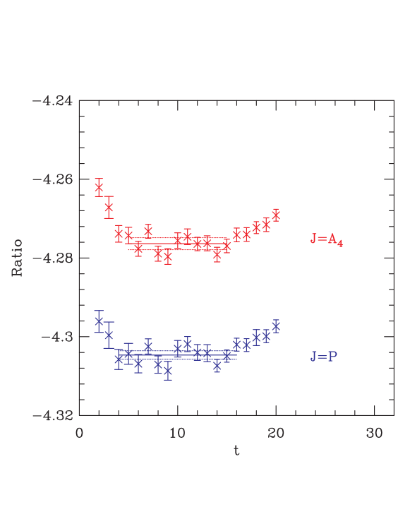
Figure 8: The ratio defined in eq. 10 for sources $J=P$ and $J=A_{4}$. Data from the 64NP set with all propagators having mass $\kappa=\kappa_{5}$.

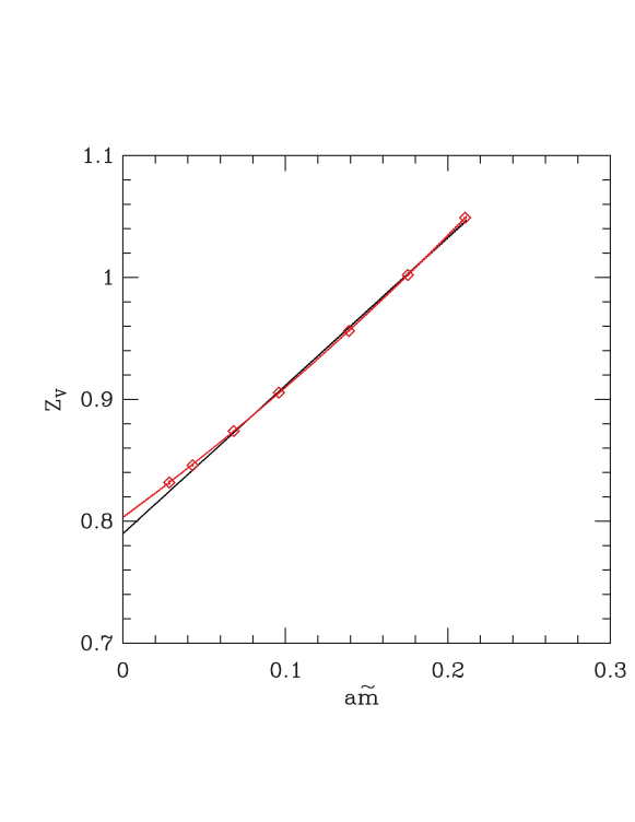
Figure 9: Linear and quadratic fit to $Z_{V}$ versus ${a\widetilde{m}}$ for the 64NP data set.

VII $c_{V}$ and $\widetilde{b}_{A}-\widetilde{b}_{V}$

Up to this stage, we have used only two-point correlation functions or three-point correlators involving the vector charge. We now turn to axial Ward identities involving three-point correlators. These allow us to determine $c_{V}$, $\widetilde{b}_{A}-\widetilde{b}_{V}$, $Z_{A}^{0}$, $Z_{P}^{0}/Z_{S}^{0}$, ${\widetilde{b}}_{P}-{\widetilde{b}}_{S}$, and $c_{T}$, as well as giving an alternate determination of $Z_{V}^{0}$. We first consider the improvement coefficient $c_{V}$ whose precise determination feeds into the calculation of $Z_{A}^{0}$, $Z_{P}^{0}/Z_{S}^{0}$, $c_{T}$, and $c_{A}^{\prime}$. The best signal for $c_{V}$ is obtained by enforcing $N_{1}=N_{2}+c_{V}D$, with

$$N_{1} = \frac{\sum_{\vec{y}}\langle\delta{\cal S}^{(12)}_{I}\ (V_{I})_{4}^{(23)}(\vec{y},y_{4})\ P^{(31)}(0)\rangle}{\sum_{\vec{y}}\langle(A_{I})_{4}^{(13)}(\vec{y},y_{4})\ P^{(31)}(0)\rangle}\,,$$ (13)

$$N_{2} = \frac{\sum_{\vec{y}}\langle\delta{\cal S}^{(12)}_{I}\ V_{i}^{(23)}(\vec{y},y_{4})\ A_{i}^{(31)}(0)\rangle}{\sum_{\vec{y}}\langle(A_{I})_{i}^{(13)}(\vec{y},y_{4})\ A_{i}^{(31)}(0)\rangle}\,,$$ (14)

$$D = \frac{\sum_{\vec{y}}\langle\delta{\cal S}^{(12)}_{I}\ a\partial_{\mu}T_{i\mu}^{(23)}(\vec{y},y_{4})\ A_{i}^{(31)}(0)\rangle}{\sum_{\vec{y}}\langle(A_{I})_{i}^{(13)}(\vec{y},y_{4})\ A_{i}^{(31)}(0)\rangle}\,,$$ (15)

so that

$$c_{V}=\frac{N}{D}\equiv\frac{N_{1}-N_{2}}{D}\,.$$ (16)

We recall that $\delta{\cal S}$ uses two-point discretization (and the corresponding value of $c_{A}(\widetilde{m}_{1})$), but that the other improved currents in these expressions are discretized both with the two- and three-point forms giving two sets of estimates. Within each set we provide two estimates using $c_{A}(0)$ and $c_{A}(m)$ in the expression for $A_{I}$. We also recall that we always use $\widetilde{m}_{1}=\widetilde{m}_{2}$.

Figures 10, 11 and 12 illustrate the quality of our data for $N_{1}$, $N_{2}$ and $D$. The improvement in errors and overall quality as $\beta$ increases is evident. Note that $N_{2}$ and $D$ are expected to have larger errors than $N_{1}$ since the lightest state which contributes is the axial-vector rather than the pion.

Our procedure is to determine $N_{1}$, $N_{2}$ and $D$ from fits to the plateaus and then combine the first two to form $N\equiv N_{1}-N_{2}$. The results for $N$ and $D$ at $\beta=6.4$ are shown in Fig. 13, where it is apparent that the errors in $N$ determine the quality of the result for $c_{V}=N/D$. As noted in Ref. Bhattacharya et al., 2001 for the data at $\beta=6$ and $6.2$, both $N$ and $D$ are to good approximation functions of $\widetilde{m}_{1}-\widetilde{m}_{3}$ that vanish when $\widetilde{m}_{1}\approx\widetilde{m}_{3}$. Since they do not, however, vanish at exactly the same point (presumably due to statistical and residual discretization errors), their ratio diverges, as shown in Fig. 14.

In Ref. Bhattacharya et al., 2001, we used three methods to extract $c_{V}$ that try to minimize the effect of this spurious singularity, and we follow the same strategy here. Details of the methods will not, however, be repeated. Our estimates at $\beta=6.0$ and $6.2$ have changed after redoing the chiral fits to $N_{1}$, $N_{2}$ and $D$, and so we quote, in Table 5, results for all $\beta$. For each method we have an additional four choices: we can use two-point or three-point discretization of the currents, and for each of these we can use either mass-dependent or chirally extrapolated values of $c_{A}$ in the operator $(A_{I})_{4}^{(13)}$ appearing in the denominator of $N_{1}$.

The extrapolation method has the largest uncertainty so we discard it. The consistency between the result using the “$1/m$ fit”, shown in Fig. 14, and the “slope-ratio” method, improves with $\beta$, but the “slope-ratio” method is more stable with respect to the range of quark masses used in the fits at all three $\beta$ values, and has the smallest dependence on the choice of $c_{A}$. We therefore take our final estimates from the “slope-ratio” method and average the $c_{A}(\widetilde{m})$ and $c_{A}(\widetilde{m}=0)$ values to get our final estimates. As usual, we take the central value from the two-point scheme and use the three-point scheme to estimate the discretization error.

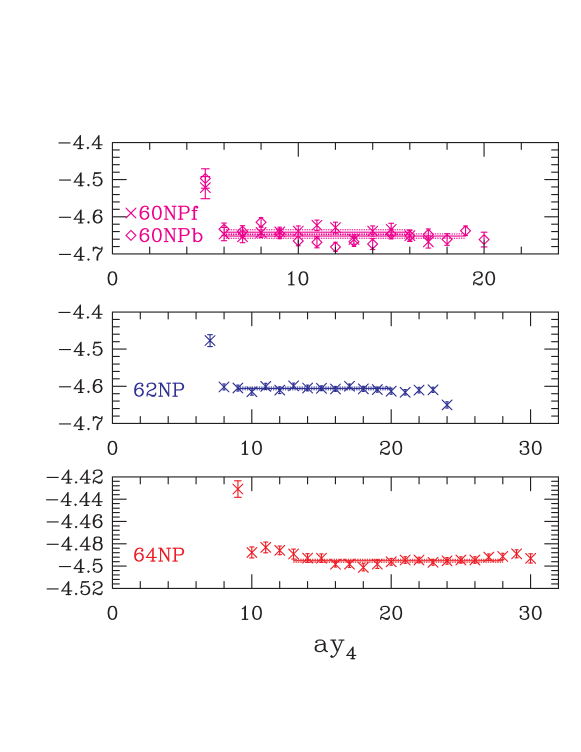
Figure 10: Illustration of the quality of the signal for the quantity $N_{1}$ of Eq. (13) for all four data sets with two-point discretization and $c_{A}(\widetilde{m})$. In all cases the data have to be multiplied by the respective values of $2\kappa_{3}$, the lattice normalization of the additional propagator in the numerator.

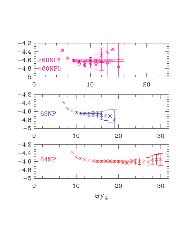
Figure 11: Illustration of the quality of the signal for $N_{2}$ of Eq. (14) for all four data sets with two-point discretization and $c_{A}(\widetilde{m})$. In all cases the data are for $\kappa_{3}$ and have to be multiplied by the respective values of $2\kappa_{3}$, the lattice normalization of the additional propagator in the numerator.

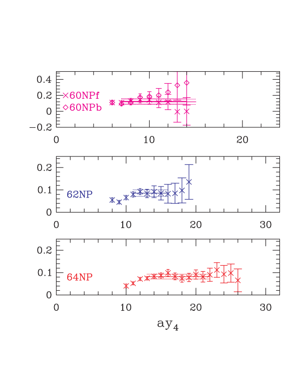
Figure 12: Illustration of the quality of the signal for $D$ of Eq. (15) for all four data sets with two-point discretization and $c_{A}(\widetilde{m})$, using $\kappa_{3}$ propagators in all cases.

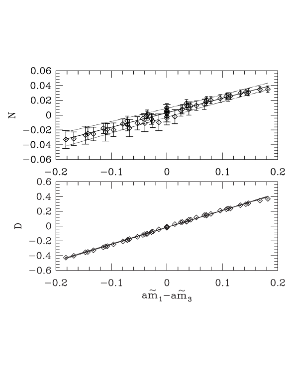
Figure 13: Data for $N$ and $D$, defined in the text and used to extract $c_{V}$, plotted as a function of ${\widetilde{m}}_{1}-{\widetilde{m}}_{3}$ for the 64NP dataset with two-point discretization and $c_{A}(\widetilde{m})$.

Figure 14: A fit of the form $c_{V}=c_{V}^{(0)}+c_{V}^{(1)}/({\widetilde{m}}_{1}-{\widetilde{m}}_{3})$ to the 64NP data with two-point discretization and $c_{A}(\widetilde{m})$.

We can also use the quantity $N_{1}$, defined in Eq. 13, to determine ${\widetilde{b}}_{A}-{\widetilde{b}}_{V}$, $b_{V}-b_{A}$ and to give an alternate determination of $Z_{V}^{0}$. We must first extrapolate to $\widetilde{m}_{1}=\widetilde{m}_{2}=0$ to remove the contribution of equations-of-motion operators. In Fig. 15 we illustrate the quadratic fits used to do this for the 64NP data. We then fit to a quadratic function of $\widetilde{m}_{3}$ or $m_{3}$. These fits, shown in Fig. 16 for two-point discretization and $c_{A}(0)$, have parameters

$$\frac{1}{Z_{V}^{0}}\big{(}1+({\widetilde{b}}_{A}-{\widetilde{b}}_{V})\frac{a{\widetilde{m}}_{3}}{2}+O(a^{2})\big{)} = 1.249(3)\big{(}1-0.123(54)\frac{a{\widetilde{m}}_{3}}{2}+0.06(38)(\frac{a{\widetilde{m}}_{2}}{2})^{2}\big{)}$$

$$\frac{1}{Z_{V}^{0}}\big{(}1+({b}_{A}-{b}_{V})\frac{am_{3}}{2}+O(a^{2})\big{)} = 1.250(3)\big{(}1-0.130(49)\frac{am_{3}}{2}-0.25(33)(\frac{am_{3}}{2})^{2}\big{)}\,.$$ (17)

The estimates for $Z_{V}^{0}$ are consistent with those obtained using the conserved vector charge, Eq. 11, but have larger errors, so our preferred value is from the analysis presented in Section VI.

The coefficient of the term linear in $\widetilde{m}$ ($m$) gives ${\widetilde{b}}_{A}-{\widetilde{b}}_{V}$ ($b_{A}-b_{V}$). We find that the errors in both ${\widetilde{b}}_{A}-{\widetilde{b}}_{V}$ and $b_{A}-b_{V}$ are large and comparable. In addition, there can be large $O(a)$ errors feeding in from the dependence of $c_{A}$ on $\widetilde{m}$ as discussed below.

It is easy to see that when using Eq. (13) to extract $\widetilde{b}_{A}-\widetilde{b}_{V}$ the result will depend on the choice whether $c_{A}(m)$ or the chirally extrapolated $c_{A}(0)$ is used. As explained in Bhattacharya et al. (2001), a shift $c_{A}\to c_{A}+\xi$ in the definition of $(A_{I})_{4}$ in the denominator produces a change in $Z_{V}^{0}$ of the form $\xi aB_{\pi}$. If, instead, we use $c_{A}(\widetilde{m})=c_{A}+\Delta\widetilde{m}a$ in the calculation then the slope, not the intercept, changes, i.e., one gets $\widetilde{b}_{A}-\widetilde{b}_{V}-\Delta aB_{\pi}/2$ instead of $\widetilde{b}_{A}-\widetilde{b}_{V}$. For the two-point data at $\beta=6.4$ the two estimates are $-0.32(5)$ and $-0.12(5)$ for $c_{A}(\widetilde{m})$ and $c_{A}(0)$ respectively. The difference, $\sim 0.20$, even though formally of higher order in $a$, is large because $aB_{\pi}\sim 1.5$ and $\Delta=0.19$ as discussed in the extraction of $c_{A}$. We do not have an a priori argument that, to this order, favors one choice over another. Anticipating that calculations of physical quantities will use improvement constants defined in the chiral limit and understanding that the slope $\Delta$ is almost entirely an artifact of the discretization scheme used to calculate $c_{A}$, we take results obtained using $c_{A}(m=0)$ for the two-point discretization as our estimates. We stress that we do not include the difference between the results using $c_{A}(m)$ and $c_{A}(0)$ as part of the error. These new results supercede those given in Bhattacharya et al. (2001).

Overall, ${\widetilde{b}}_{A}-{\widetilde{b}}_{V}$ is small and the uncertainty is comparable to the signal. The expected relation $({\widetilde{b}}_{A}-{\widetilde{b}}_{V})=(Z_{A}^{0}Z_{S}^{0}/Z_{P}^{0})(b_{A}-b_{V})+O(a)$ holds at the $1\sigma$ level.

Figure 15: Quadratic extrapolation of the ratio in Eq. (13) in $\widetilde{m}_{1}=\widetilde{m}_{2}$ for fixed $\widetilde{m}_{3}=\kappa_{4}$ for 64NP data set with two-point discretization and $c_{A}(\widetilde{m})$.

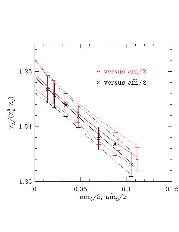
Figure 16: Quadratic fits to Eq. (13) to extract ${\widetilde{b}}_{A}-{\widetilde{b}}_{V}$ and $b_{A}-b_{V}$ for 64NP data set with two-point discretization and $c_{A}(\widetilde{m})$. The crosses show data and fits versus the AWI quark mass $\widetilde{m}$, whereas the diamonds show results obtained using the VWI quark mass $m$.

VIII $Z_{A}^{0}$

The Ward identity

$$\frac{\sum_{\vec{y}}\langle\delta{\cal S}^{(12)}_{I}\ (A_{I})_{i}^{(23)}(\vec{y},y_{4})\ V_{i}^{(31)}(0)\rangle}{\sum_{\vec{y}}\langle(V_{I})_{i}^{(13)}(\vec{y},y_{4})\ V_{i}^{(31)}(0)\rangle} = \frac{Z_{V}^{0}(1+\widetilde{b}_{V}a\widetilde{m}_{3}/2)}{Z_{A}^{0}\cdot Z_{A}^{0}(1+\widetilde{b}_{A}a\widetilde{m}_{3}/2)}\,,$$ (18)

gives $Z_{V}^{0}/(Z_{A}^{0})^{2}$ and a second estimate of ${\widetilde{b}}_{A}-{\widetilde{b}}_{V}$. The quality of the signal for the ratio of correlation functions, as illustrated in Fig. 17, is good as the intermediate state is the vector meson. Data in Fig. 18 show that quadratic fits in both $\widetilde{m}_{1}\equiv\widetilde{m}_{2}$ and $\widetilde{m}_{3}$ are preferred at $\beta=6.4$. Linear fits are sufficient at $\beta=6.0$ and $6.2$. The resulting values are given in Tables 3 and 4.

Including the results in Section VI we have two estimates for ${\widetilde{b}}_{A}-{\widetilde{b}}_{V}$ with similar errors. These estimates come from Ward identities that involve different, pseudoscalar versus vector, intermediate states. Also, in Eq. 18 the term proportional to $c_{A}$ in $A_{I}$ does not contribute at zero momentum so there is no associated uncertainty. Thus, the $O(a)$ errors can be different in the two cases. As shown in Tables  3 and 4, we find that the two estimates show considerable $O(a)$ variation, but this is not unexpected given the size of the errors and the possibility of additional $O(a\Lambda_{QCD}\sim 0.2-0.1)$ uncertainty in previous estimates as discussed in Section VI. Had we chosen to use $c_{A}(\widetilde{m})$ to extract ${\widetilde{b}}_{A}-{\widetilde{b}}_{V}$ in Section VI the variation would have been larger by a factor of two or more. Thus, for our final estimate we average the two two-point estimates and quote the difference between two-point and three-point discretization schemes as an estimate of residual $O(a)$ errors. The upshot of the analysis is that ${\widetilde{b}}_{A}-{\widetilde{b}}_{V}$ is small and the systematic errors are of the same size as the signal.

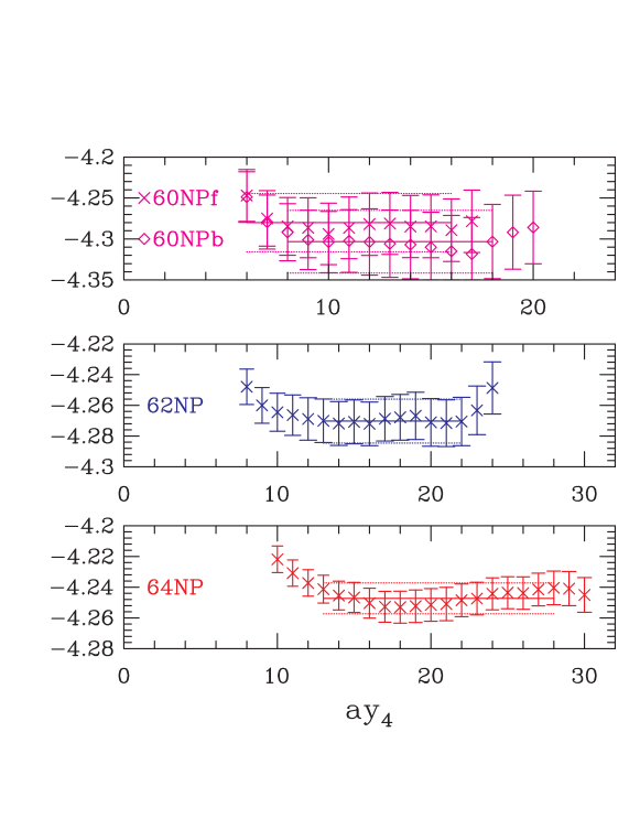
Figure 17: Illustration of the signal for the ratio defined in Eq. (18) for the four data sets using two-point discretization. In all four cases the data have to be multiplied by the respective values of $2\kappa_{3}$, the lattice normalization of the additional propagator in the numerator.

Figure 18: The 64NP two-point data for $Z_{V}/Z_{A}^{0}Z_{A}(\widetilde{m}_{3})$ are obtained by extrapolating the ratio defined in Eq. 18 to $\widetilde{m}_{1}=\widetilde{m}_{2}=0$ using a quadratic fit. The intercept of the quadratic fit in $\widetilde{m}_{3}$, gives $Z_{V}^{0}/Z_{A}^{0}Z_{A}^{0}$.

To estimate $Z_{A}^{0}$ we use the product of Eqs. (18) and (13) as it yields $1/(Z_{A}^{0})^{2}$ directly. The final chiral extrapolation in $a\widetilde{m}_{3}$ for the product is shown in Fig. 19. In this product the terms proportional to $a\widetilde{m}_{3}$ cancel, but nevertheless the data show a clear $a\widetilde{m}_{3}$ dependence. This we interpret as due to $O(a^{2})$ terms of the generic form $Z_{A}^{0}(\widetilde{m}_{3})=Z_{A}^{0}(0)(1+a^{2}\widetilde{m}_{3}\Lambda)$. The slopes at $\beta=6.0$, $6.2$ and $6.4$ are $0.22(6)$, $0.12(11)$ and $0.11(4)$ respectively. To match the observed slope $a\Lambda\approx 0.11$ at $\beta=6.4$ requires $\Lambda\sim\Lambda_{QCD}\approx 0.4\;$GeV, which is a reasonable value. Also, the change between $\beta=6.0$ and $6.4$ is consistent with the expected scaling in $a$. In Ref. Bhattacharya et al. (2001) we had ignored this dependence and fit the data to a constant to extract $Z_{A}^{0}$. In light of our results at $\beta=6.4$ and a better understanding of possible $\widetilde{m}_{3}$ dependence, we have refit the data at $\beta=6.0$ and $6.2$ also. We now use quadratic extrapolation in $\widetilde{m}_{1}\equiv\widetilde{m}_{2}$ at $\beta=6.4$ and linear at $\beta=6.0$ and $6.2$. Linear extrapolation in $\widetilde{m}_{3}$ works well at all three couplings, however at $\beta=6.2$ and $6.4$ we use quadratic fits to maintain consistency with the rest of the analysis. At these weaker couplings linear and quadratic estimates are consistent.

A comparison of Figs. 18 and 19 raises the following concern. The slope in Fig. 18 with respect to $a\widetilde{m}_{3}$ relative to the intercept is an $O(a)$ effect, proportional to $\widetilde{b}_{V}-\widetilde{b}_{A}$, while that in Fig. 19 is, as just discussed, of one higher order. The two slopes are, however, numerically very similar. This once again suggests that there can be substantial uncertainty of $O(a)$, comparable to the value itself, in any result for $\widetilde{b}_{V}-\widetilde{b}_{A}$. In fact, our analysis illustrates a problem common to the extraction of all measurements of the differences $b_{{\cal O}}-b_{\delta\cal O}$. The signal, the errors, and the $O(a^{2}m\Lambda)$ uncertainties are all comparable.

Figure 19: $Z_{A}^{0}$ is obtained from the product of ratios of correlators defined in Eqs. (18) and (13). The figure shows a quadric extrapolation in ${\widetilde{m}}_{3}/2$ for the 64NP data set with two-point discretization and $c_{A}(\widetilde{m})$.

IX $Z_{P}^{0}/Z_{S}^{0}$, $\widetilde{b}_{P}-\widetilde{b}_{S}$

To obtain $Z_{P}^{0}/(Z_{S}^{0}Z_{A}^{0})$ and ${\widetilde{b}}_{P}-{\widetilde{b}}_{S}$ we use the identity

$$\frac{\sum_{\vec{y}}\langle\delta{\cal S}^{(12)}_{I}\ S^{(23)}(\vec{y},y_{4})\ J^{(31)}(0)\rangle}{\sum_{\vec{y}}\langle P^{(13)}(\vec{y},y_{4})\ J^{(31)}(0)\rangle} = \frac{Z_{P}^{0}(1+\widetilde{b}_{P}a\widetilde{m}_{3}/2)}{Z_{A}^{0}\cdot Z_{S}^{0}(1+\widetilde{b}_{S}a\widetilde{m}_{3}/2)}\,,$$ (19)

evaluated in the limit $\widetilde{m}_{1}\equiv\widetilde{m}_{2}\to 0$ with $J=P$ or $A_{4}$. The intermediate state in both the numerator and the denominator has the quantum numbers of a pion, and the ratio has a very good signal, whose quality, as a function of $\beta$, is shown in Fig. 20. Data at $\beta=6.4$ for the ratio on the left hand side of Eq. (19) favor quadratic fits for $\widetilde{m}_{1}\equiv m_{2}\to 0$ and $\widetilde{m}_{3}\to 0$ extrapolations as illustrated in Figure 21. The intercept and the slope give $Z_{P}^{0}/(Z_{S}^{0}Z_{A}^{0})$ and ${\widetilde{b}}_{P}-{\widetilde{b}}_{S}$ respectively, and these estimates are quoted in Tables 3 and 4. To get $Z_{P}^{0}/Z_{S}^{0}$ we eliminate $Z_{A}^{0}$ by combining the ratio in Eq. (19) with the product of Ward identities discussed in section VIII.

The value of ${\widetilde{b}}_{P}-{\widetilde{b}}_{S}$ is numerically small, comparable to the errors and of the same order as $O(a^{2}m_{3}\Lambda)$ effects discussed in Section VIII. In this case we take the average of the two-point and three-point values as our best estimate. The reason is that the operators in Eq. (19) do not contain any derivatives (no improvement terms) so the difference between two-point and three-point estimates arises solely from the chiral extrapolations due to the tiny differences in $\widetilde{m}$ for the two cases as shown in Table 8.

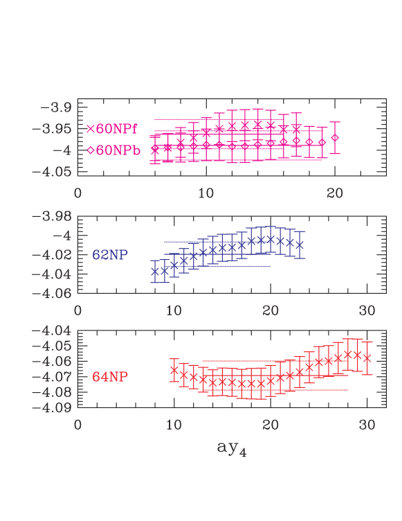
Figure 20: Comparison of the signal in the ratio of correlators on the l.h.s. of Eq. (19) used to extract $Z_{P}^{0}/Z_{S}^{0}$. In all four cases the data have to be multiplied by the respective values of $2\kappa_{3}$, the lattice normalization of the additional propagator in the numerator.

Our results for $Z_{P}^{0}/Z_{S}^{0}$, obtained using Eq. (19) and $Z_{A}$ from Section VIII, are presented in Table 6. These are consistent with the recent estimates by the ALPHA and SPQcdR collaborations Becirevic et al. (2004). In Section XIV we compare our results with predictions of one-loop perturbation theory and discuss the size of $O(a^{2})$ and $O(\alpha_{s}^{2})$ corrections needed to explain the large difference.

X $Z_{P}^{0}/(Z_{S}^{0}Z_{A}^{0})$, $\widetilde{b}_{A}-\widetilde{b}_{P}-\widetilde{b}_{m}$, and $\widetilde{b}_{m}$

One can derive a relation between the two definitions of quark mass de Divitiis and Petronzio (1998),

$$\frac{\widetilde{m}}{m}=\frac{Z_{P}^{0}Z_{m}^{0}}{Z_{A}^{0}}[1-(\widetilde{b}_{A}-\widetilde{b}_{P}-\widetilde{b}_{m})a{\widetilde{m}}_{av}+\widetilde{b}_{m}a\frac{({\widetilde{m}}^{2})_{av}-({\widetilde{m}}_{av})^{2}}{{\widetilde{m}}_{av}}+O(a\widetilde{m})^{2}]\,,$$ (20)

where ${X}_{av}=(X_{1}+X_{2})/2$. This relation is useful because $Z_{m}^{0}=1/Z_{S}^{0}$ and $b_{S}=-2b_{m}$ Lüscher ; Bhattacharya et al. (2006).

In Fig. 21 we illustrate fits to Eq. (20) for the simpler case of degenerate quarks for $\widetilde{m}$ calculated using both $c_{A}(\widetilde{m})$ and $c_{A}(0)$. In this case the term proportional to $\widetilde{b}_{m}$ does not contribute. The data show that for $\beta=6.4$ including a term quadratic in ${\widetilde{m}}_{av}$ gives a much better fit whereas for $6.0$ and $6.2$ a linear fit suffices. The term proportional to $b_{m}$ contributes only to non-degenerate combinations. Fits using all combinations of six ($\beta=6.0)$ and seven ($\beta=6.2$ and $6.4$) values of quark masses allow both $\widetilde{b}_{P}-\widetilde{b}_{A}-{\widetilde{b}}_{m}$ and ${\widetilde{b}}_{m}$ to be extracted reliably. These two sets of results of the fits, using $c_{A}(\widetilde{m})$ and $c_{A}(0)$, are quoted in Tables 3 and 4.

The intercept, which gives ${Z_{P}^{0}}/{Z_{A}^{0}Z_{S}^{0}}$, should be same for $c_{A}(m)$ and $c_{A}(0)$, to the extent that the fits are good. Furthermore, the difference between two- and three-point results (which have different results for $c_{A}$) should be small. These features are borne out by the results. The only notable difference is that the errors in the two-point data are smaller. The results are also consistent with those obtained using Eq. (19), and have similar errors, as illustrated in Fig. 21. In Ref. Bhattacharya et al. (2001) we preferred the results from Eq. (19) since the method of this section has a greater sensitivity to uncertainties in $c_{A}$ (which are enhanced by the presence of the factor $B_{\pi}=M_{\pi}^{2}/\widetilde{m}\approx 4\;$GeV). With better understanding of the errors we now choose to take, for our final value of ${Z_{P}^{0}}/{Z_{A}^{0}Z_{S}^{0}}$, the weighted mean of the two-point results from Eq. (19) and those using $\widetilde{m}/m$, with the latter determined using $c_{A}(\widetilde{m})$.

The extraction of $\widetilde{b}_{A}-\widetilde{b}_{P}+\widetilde{b}_{S}/2$ and $\widetilde{b}_{S}$ is effected by the choice of $c_{A}$. Using Eqs. 7 and 20 one can show that, to leading order, $(\widetilde{b}_{A}-\widetilde{b}_{P}+\widetilde{b}_{S}/2)|_{c_{A}(m)}=(\widetilde{b}_{A}-\widetilde{b}_{P}+\widetilde{b}_{S}/2)|_{c_{A}(0)}-\Delta aB_{\pi}/2$ and similarly for $\widetilde{b}_{m}$. Our data are roughly consistent with this relation for both the two-point and three-point discretization methods. For example, in case of the two-point discretization method, the values of the slope $\Delta$, illustrated in Fig. 5 for $\beta=6.4$ data, are approximately $0.18$, $0.18$ and $0.19$ and $aB_{\pi}\approx 2.6$, $1.9$ and $1.5$ at the three couplings respectively. This $O(a)$ effect, enhanced by the large value of $B_{\pi}$, gives rise to the difference in slopes as illustrated in Fig. 21.

For the two combination of $b$’s the two-point and three-points results are consistent for $c_{A}(\widetilde{m})$. This is expected because, as discussed in section IV, at each quark mass the $\widetilde{m}$ extracted from the two discretization schemes are, up to $O(a^{3})$, the same, provided the mass dependent $c_{A}(m)$ are used. We also find that the fits to two-point data with $c_{A}(m)$ are marginally better. So we use estimates obtained from the two-point data with $c_{A}(\widetilde{m})$ for the central values.

Note that the considerations regarding choice of $c_{A}(\widetilde{m})$ versus $c_{A}(0)$ here are different from those applied in section VII when determining $\widetilde{b}_{A}-\widetilde{b}_{V}$. To avoid confusion it is worthwhile summarizing our choices. The quark mass $\widetilde{m}$ and $c_{A}(\widetilde{m})$ are extracted simultaneously from the two-point AWI. We then use these $\widetilde{m}$ and $c_{A}(\widetilde{m})$ in all calculations of $\delta S$. For improving the external current, $A_{I}$, in the three-point AWI we use $c_{A}(0)$. Lastly, the “slope-ratio” method, where we use the average of data with $c_{A}(\widetilde{m})$ and $c_{A}(0)$, gives $c_{V}(0)$ needed to improve the vector current.

The estimate of $\widetilde{b}_{A}-\widetilde{b}_{P}+\widetilde{b}_{S}/2$ from fits to Eq. 20 using the full set of masses (degenerate and non-degenerate) is very similar to that obtained using only the degenerate set. Including non-degenerate combinations we find that $\widetilde{b}_{m}$ can also be extracted reliably. With $\widetilde{b}_{A}-\widetilde{b}_{P}+\widetilde{b}_{S}/2$ and $\widetilde{b}_{S}$ in hand we can finally extract $\widetilde{b}_{P}$ in two ways. The first is obtained by combining $\widetilde{b}_{P}-\widetilde{b}_{S}$ and $\widetilde{b}_{S}$ and the second combines $\widetilde{b}_{V}$, $\widetilde{b}_{A}-\widetilde{b}_{V}$, $\widetilde{b}_{A}-\widetilde{b}_{P}+\widetilde{b}_{S}/2$ and $\widetilde{b}_{S}$. Both estimates use one combination of $b$’s from the three-point axial Ward identity. These are of similar quality and dominate the errors. We find that these two estimates of $\widetilde{b}_{P}$, which provide a consistency check, differ at the level of the uncertainties present in all combinations of $b$’s extracted using three-point AWI. For our final estimates of $\widetilde{b}_{P}$ given in table 6 we take the weighted average.

Figure 21: Quadratic fits used to extract $Z_{A}^{0}Z_{S}^{0}/Z_{P}^{0}$. The three fits correspond to (i) Eq. (19) plotted versus $a\widetilde{m}=a\widetilde{m}_{3}/2$, (ii) Eq. (20) with $\widetilde{m}$ defined using the mass dependent $c_{A}$, and (iii) Eq. (20) with $\widetilde{m}$ defined using the chirally extrapolated $c_{A}$. The data are from the 64NP set with two-point discretization. Note that the intercepts from all three fits should agree up to errors of $O(a^{2})$, but the slope of (i) is $b_{P}-b_{S}$ whereas those of (ii) and (iii) give ${\widetilde{b}}_{A}-{\widetilde{b}}_{P}-{\widetilde{b}}_{m}$.

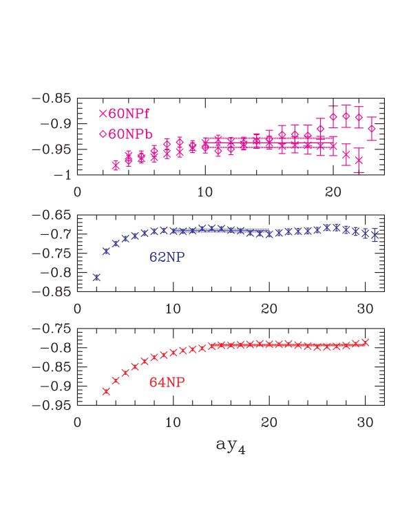
Figure 22: The signal in the ratio of correlators used to extract $c_{T}$ and defined on the left hand side of Eq. (21). The points are from 64NP two-point data with $\kappa_{3}$ quark propagators.

XI $c_{T}$

$c_{T}$ is extracted by solving, for each ${\widetilde{m}}_{3}$, the Ward identity

$$1+ac_{T}\frac{\sum_{\vec{y}}\langle[-\partial_{4}V_{k}]^{(13)}(\vec{y},y_{4})T_{k4}^{(31)}(0)\rangle}{\sum_{\vec{y}}\langle T_{k4}^{(13)}(\vec{y},y_{4})T_{k4}^{(31)}(0)\rangle} = Z_{A}^{0}\frac{\sum_{\vec{y}}\langle\delta{\cal S}^{(12)}_{I}\ T_{ij}^{(23)}(\vec{y},y_{4})\ T_{k4}^{(31)}(0)\rangle}{\sum_{\vec{y}}\langle T_{k4}^{(13)}(\vec{y},y_{4})\ T_{k4}^{(31)}(0)\rangle}\,,$$ (21)

and extrapolating these estimates to $\widetilde{m}_{3}=0$ as discussed in Ref. Bhattacharya et al., 2001. The quality of the data for the ratios on the left and right hand sides of this equation is very good as illustrated in Figs. 22 and 23. We find that the two-point and three-point methods give consistent estimates after the chiral extrapolations. We take the two-point value as our final estimate and the difference from the three-point result as a systematic uncertainty.

The data, illustrated in Fig. 24, exhibit a behavior linear in $\widetilde{m}_{3}$. This can arise due to corrections of the form $O(a\Lambda a\widetilde{m}_{3})$. We had erroneously neglected this $O(\widetilde{m}_{3}a)$ dependence in $c_{T}$ in previous analyses. The slopes, $-0.33(11)$, $-0.21(10)$ and $-0.17(3)$ at $\beta=6.0$, $6.2$ and $6.4$ respectively, are consistent with an $a\Lambda$ behavior. The change in $c_{T}$ between a constant and a linear fit are significant at the $1\sigma$ level, $i.e.$ they change from $0.063(7)\to 0.085(12)$, $0.051(7)\to 0.063(10)$, $0.041(3)\to 0.054(5)$ for the three $\beta$ values respectively. Thus, our new estimates, based on linear fits, differ from those quoted in Ref. Bhattacharya et al., 2001.

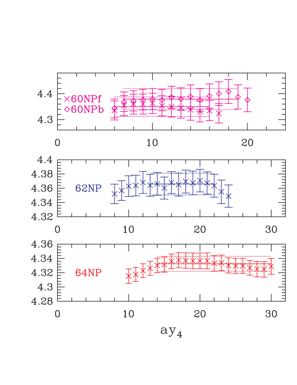
Figure 23: The signal in the ratio of correlators defined on the right hand side of Eq. (21). This 64NP data are used to extract $c_{T}$. In all four cases the data have to be multiplied by the respective values of $2\kappa_{3}$, the lattice normalization of the additional propagator in the numerator.

Figure 24: $c_{T}$ is extracted using a quadratic fit to all seven quark masses ($\kappa_{1}-\kappa_{7}$) for the 64NP data set with two-point discretization and $c_{A}(\widetilde{m})$.

XII Equation-of-motion operators

We extract the coefficients, $c^{\prime}_{\cal O}$, of the equation-of-motion operators from the $\widetilde{m}_{12}$ dependence of the three-point AWI Bhattacharya et al. (2001):

$$\frac{\langle\int_{V}d^{4}x\,\delta S_{I}^{(12)}\ {\cal O}_{I}^{(23)}(y_{4},\vec{y})\ J^{(31)}(0)\rangle}{\langle\delta{\cal O}_{I}^{(13)}(y_{4},\vec{y})\ J^{(31)}(0)\rangle}=\frac{Z^{(13)}_{\delta{\cal O}}}{Z^{(12)}_{A}\ Z^{(23)}_{\cal O}}+a\frac{c^{\prime}_{P}+c^{\prime}_{\cal O}}{2}{\widetilde{m}}_{12}+O(a^{2})\,.$$ (22)

This can be rewritten as

$$c^{\prime}_{P}+c^{\prime}_{\cal O}=2s_{\cal O}-X_{\cal O}\big{(}\widetilde{b}_{\delta{\cal O}}-\widetilde{b}_{\cal O}-2\widetilde{b}_{A}\big{)}\,,$$ (23)

where $X_{\cal O}={Z^{0}_{\delta{\cal O}}}/{Z^{0}_{A}\ Z^{0}_{\cal O}}$ and $s_{\cal O}$ is the slope, in the limit $\widetilde{m}_{3}\to 0$, of the left hand side of Eq. (22) with respect to $\widetilde{m}_{1}$ for fixed $\widetilde{m}_{3}$. The results for $c^{\prime}_{P}+c^{\prime}_{\cal O}$ are shown in Table 7, and for the three individual pieces $s_{\cal O}$, $X_{\cal O}(b_{\delta{\cal O}}-b_{{\cal O}})/2$, and $X_{\cal O}b_{A}$ in Table 10.

$62NP$
$c^{\prime}_{\cal O}+c^{\prime}_{P}$	$s_{\cal O}$	$X_{\cal O}(b_{\delta{\cal O}}-b_{{\cal O}})/2$	$X_{\cal O}b_{A}$
$c^{\prime}_{V}+c^{\prime}_{P}$	$-0.22(05)$	$-0.06(2)$	$1.50(5)$
$c^{\prime}_{A}+c^{\prime}_{P}$	$-0.15(07)$	$+0.05(5)$	$1.42(5)$
$c^{\prime}_{P}+c^{\prime}_{P}$	$-0.17(10)$	$-0.11(6)$	$1.56(6)$
$c^{\prime}_{S}+c^{\prime}_{P}$	$-0.15(03)$	$-0.05(1)$	$1.29(5)$
$c^{\prime}_{T}+c^{\prime}_{P}$	$-0.21(07)$	$+0.02(5)$	$1.45(5)$
$64NP$
$c^{\prime}_{\cal O}+c^{\prime}_{P}$	$s_{\cal O}$	$X_{\cal O}(b_{\delta{\cal O}}-b_{{\cal O}})/2$	$X_{\cal O}b_{A}$
$c^{\prime}_{V}+c^{\prime}_{P}$	$-0.18(5)$	$-0.08(3)$	$1.36(6)$
$c^{\prime}_{A}+c^{\prime}_{P}$	$-0.08(6)$	$+0.08(4)$	$1.27(6)$
$c^{\prime}_{P}+c^{\prime}_{P}$	$-0.84(36)$	$-0.41(32)$	$1.49(8)$
$c^{\prime}_{S}+c^{\prime}_{P}$	$-0.06(4)$	$-0.06(3)$	$1.18(6)$
$c^{\prime}_{T}+c^{\prime}_{P}$	$-0.17(7)$	$-0.05(5)$	$1.31(6)$

Table 10: The three contributions to the coefficient of the equation of motion operators $c^{\prime}_{\cal O}+c^{\prime}_{P}$ for the 62NP and 64NP data sets using the two-point derivative data and $c_{A}(\widetilde{m})$ in the calculation of $\delta S$ and $c_{A}(0)$, $c_{V}(0)$, $c_{T}(0)$ in the discretization of the operators.

The quality of all the results is dominated by how well we can measure $c^{\prime}_{P}$. Unfortunately, the intermediate state in the relevant correlation functions is a scalar which has a poor signal. To obtain a flat region with respect to the time slice of the operator insertion we fit the ratio on the $l.h.s.$ of Eq. 22 allowing $\widetilde{m}$ in $\delta S$ to be a free parameter. The resulting $\widetilde{m}$ differ from those obtained using Eq. 7 by about $7\%$, $4\%$, and $2\%$ at $\beta=6.0$, $6.2$ and $6.4$ respectively.

There is an additional systematic uncertainty of $O(a)\sim 0.1$ in the determination of any slope from the chiral fits as discussed previously. This impacts the determination of all three terms $s_{\cal O}$, $X_{\cal O}(b_{\delta{\cal O}}-b_{{\cal O}})/2$ and $X_{\cal O}b_{A}$.

Examples of fits to the left hand side of Eq. 22 are shown in Fig. 25 for the 64NP data set. The estimates, at leading order, should not depend on ${\widetilde{m}}_{3}$, however, the data show higher order effects. We, therefore, use a quadratic extrapolation in ${\widetilde{m}}_{3}$ at $\beta=6.4$ and linear at $\beta=6.0$ and $6.2$ to get $s_{\cal O}$. This changes the estimates from those presented in Bhattacharya et al. (2001) and Bhattacharya et al. (2002).

There is a very significant improvement in the signal for both the individual terms and the final $c^{\prime}_{P}+c^{\prime}_{\cal O}$ as $\beta$ increases. Nevertheless, due to the uncertainties discussed above, all the $c^{\prime}$ could have additional systematic uncertainties similar to the errors quoted in Table 7, whose resolution is beyond the scope of this work. Thus, we consider our estimates as qualitative and warn the reader that the difference from the tree level value $c^{\prime}_{{\cal O}}=1$ should be used with caution.

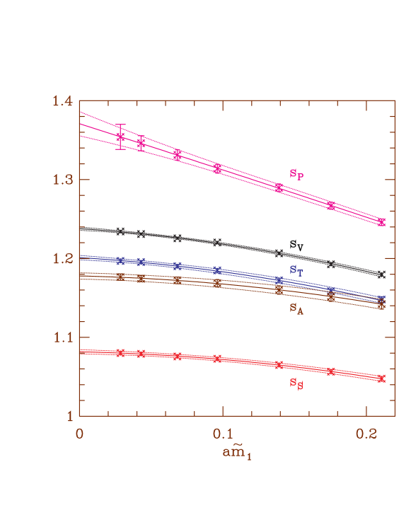
Figure 25: Quadratic fits to the l.h.s. of Eq. (22) versus $a\widetilde{m}$. The slopes $s_{\cal O}$ contribute to the coefficient of the equation of motion operators through Eq. (23). The data are for 64NP with two-point discretization, $c_{A}(\widetilde{m})$ and ${\widetilde{m}}_{3}$ chosen to be $\kappa_{3}$.

XIII Comparison with results by the ALPHA collaboration

The ALPHA collaboration has used a very different method $i.e.$, the Schrodinger Functional method, and their estimates have the largest differences from ours, so it is worthwhile comparing the two sets of values for $Z_{A}^{0}$, $Z_{V}^{0}$, $Z_{P}^{0}/Z_{S}^{0}$, $c_{A}$, $c_{V}$, and $b_{V}$. We expect the difference to vanish as $O(a^{2})$ for $Z_{A}^{0}$, $Z_{V}^{0}$ and $Z_{P}^{0}/Z_{S}^{0}$, and as $O(a)$ for $c_{A}$, $c_{V}$ and $b_{V}$. We find that, within combined errors, the estimates for $b_{V}$ by the LANL, ALPHA and QCDSF collaboration are already consistent at all three $\beta$ values as shown in Table 9. Similarly, estimates for $Z_{P}^{0}/Z_{S}^{0}$ by the LANL and ALPHA collaborations agree. For the other four quantities, there is a statistically significant difference, and we have attempted to see whether the lattice spacing dependence is consistent with theoretical expectations. To do this, we have fit the difference $\Delta X=X_{LANL}-X_{ALPHA}$ to an appropriate function of $a$, with the results:

$$\Delta Z_{V}^{0} = \phantom{-}0.004(1)-[261(16)a]^{2}\quad\chi^{2}/{ndf}=0.03$$ (24)

$$\Delta Z_{A}^{0} = -0.002(12)+[222(190)a]^{2}\quad\chi^{2}/{ndf}=0.5$$ (25)

$$\Delta c_{A} = -188(39)a+[769(74)a]^{2}\quad\chi^{2}/{ndf}=0.4$$ (26)

$$\Delta c_{V} = -0.15(14)+703(431)a\quad\chi^{2}/{ndf}=0.01$$ (27)

where $a$ is in units of MeV^-1 so that the coefficients are in units of MeV. Error estimates in $\Delta X$ were determined by adding the two independent statistical errors in quadratures. A number of comments are in order:

• These fits are very sensitive to the errors assigned to $\Delta X$ and should only be used to draw qualitative conclusions.

• As noted earlier, our condition ($m_{ij}$ independent of $t$ for $t\geq 2$) for fixing $c_{A}$, and the variation in the physical size of our sources with $a$ may lead to a more complicated dependence on $a$ than simply the leading order expectation. Similarly, we have chosen different forms for the chiral extrapolation at the various $\beta$’s. These issues have been ignored here given the small number of values of $\beta$.

• For $Z_{V}^{0}$ and $Z_{A}^{0}$ we expect a vanishing intercept and a difference proportional to $a^{2}$. This expectation is borne out reasonably well. The non-zero value for the intercept in $\Delta Z_{V}^{0}$ could be a manifestation of higher order terms that are ignored in our fit. The size of the $a^{2}$ term is consistent with being $\sim(a\Lambda_{QCD})^{2}$.

• Fits to $\Delta c_{A}$ without a quadratic term have large $\chi^{2}$. The linear plus quadratic fit given in Eq. 27 does slightly better than constant plus quadratic. The fits are dominated by the difference at $\beta=6.0$ where our estimate agrees with that given in Ref. Collins et al. (2003).

• Estimates of $c_{V}$ by the ALPHA collaboration are systematically much larger. The fit in Eq. 27 has large coefficients, however the errors are equally large. The calculation of $c_{V}$ warrants further study since the differences are large.

XIV Comparison with perturbation theory

The data at three values of the coupling allow us to also fit the difference between the non-perturbative and tadpole improved one-loop estimates as a function of $a$ and $\alpha_{s}^{2}$, $i.e.$, including both the leading order discretization and perturbative corrections. The results of these fits are

$$\Delta Z_{V}^{0} = -(192a)^{2}-(1.3\alpha_{s})^{2}\quad\chi^{2}/{ndf}=0.9$$ (28)

$$\Delta Z_{A}^{0} = -(159a)^{2}-(1.2\alpha_{s})^{2}\quad\chi^{2}/{ndf}=0.5$$ (29)

$$\Delta(Z_{P}^{0}/Z_{S}^{0}) = -(439a)^{2}-(1.9\alpha_{s})^{2}\quad\chi^{2}/{ndf}=3.5$$ (30)

$$\Delta c_{V} = -(138a)-(1.5\alpha_{s})^{2}\quad\chi^{2}/{ndf}=0.4$$ (31)

$$\Delta c_{A} = (30a)-(1.4\alpha_{s})^{2}\quad\chi^{2}/{ndf}=0.01$$ (32)

$$\Delta c_{T} = (130a)+(0.4\alpha_{s})^{2}\quad\chi^{2}/{ndf}=0.1$$ (33)

$$\Delta{\widetilde{b}_{V}} = (1197a)-(3.8\alpha_{s})^{2}\quad\chi^{2}/{ndf}=3.2$$ (34)

$$\Delta b_{V} = (630a)-(1.8\alpha_{s})^{2}\quad\chi^{2}/{ndf}=6.3$$ (35)

$$\Delta{\widetilde{b}_{A}} = -(770a)-(3.5\alpha_{s})^{2}\quad\chi^{2}/{ndf}=0.8$$ (36)

$$\Delta{\widetilde{b}_{P}} = -(857a)-(1.9\alpha_{s})^{2}\quad\chi^{2}/{ndf}=2.3$$ (37)

$$\Delta{\widetilde{b}_{S}} = (507a)-(2.3\alpha_{s})^{2}\quad\chi^{2}/{ndf}=8.9$$ (38)

where $a$ is expressed in MeV^-1, $\Delta X=X_{LANL}-X_{1-loop}$, and $\alpha_{s}=g^{2}/(4\pi u_{0}^{4})$ is the tadpole improved coupling with values $0.1340$, $0.1255$ and $0.1183$ at the three $\beta$. The tadpole factor $u_{0}$ is chosen to be the fourth root of the expectation value of the plaquette.

One conclusion from these fits is that one-loop tadpole improved perturbation theory estimates of the $Z$’s and $c$’s underestimate the corrections. The deviations can, however, be explained by coefficients of reasonable size, $i.e.$ the coefficient of $O(a)$ is $\approx\Lambda_{QCD}$ and the perturbative corrections are $(1-2)\alpha_{s}^{2}$. The case of $Z_{P}^{0}/Z_{S}^{0}$ is marginal, and we point to non-perturbative calculations using external quark and gluon states (the RI/MOM method) that show that the majority of the difference comes from 1-loop perturbation theory significantly underestimating ($1-Z_{P}^{0}$) Becirevic et al. (2004).

The most striking differences from perturbation theory are for the $b$’s. We stress, however, that the fits are very poor as evident from the $\chi^{2}/{ndf}$. There are two useful statements we can make. In the case of ${b_{V}}$ (and similarly ${\widetilde{b}}_{V}$), the agreement between our results and those by the ALPHA, QCDSF, and SPQcdR collaborations Lüscher et al. (1997a); Bakeyev et al. (2004); Becirevic et al. (2004), suggests that 1-loop perturbation theory underestimates the correction. Second, at $\beta=6.4$ ${\widetilde{b}_{A}}$, ${b_{A}}$, ${\widetilde{b}_{P}}$ and ${\widetilde{b}_{S}}$ are in good agreement with perturbation theory.

XV Conclusion

We have presented new results for renormalization and improvement constants of bilinear operators at $\beta=6.4$. Combining these with our previous estimates at $\beta=6.0$, and $6.2$, and with the results from the ALPHA collaboration we are able to quantify residual discretization errors. Overall, we find that the efficacy of the method improves very noticeably with the coupling $\beta$. Using data at $\beta=6.4$ we are able to resolve higher order mass dependent corrections in the chiral extrapolation for all the renormalization and improvement constants presented here. Our final results are summarized in Table 6.

Determination of $c_{A}$ is central to $O(a)$ improved calculations. By comparing results from three different discretization schemes we improve the reliability of our error estimate. We also show that reliable estimates from correlators at finite momenta can be extracted and find that these give consistent results with those from zero-momentum correlators once additional $O(p^{2}a^{2})$ errors are taken into account.

We find that both $c_{A}$ and $c_{V}$ are small, and the most significant differences from estimates by the ALHPA collaboration are at the strongest coupling $\beta=6.0$.

We also compare our non-perturbative estimates with one-loop tadpole improved perturbation theory. Overall, we find estimates based on 1-loop tadpole improved perturbation theory underestimate the corrections in the $Z$’s and $c$’s. The differences can, however, be explained by terms of $O(\Lambda_{QCD}a)$ and $(1-2)\alpha_{s}^{2}$.

The most significant differences are in $b_{V}$ and $\widetilde{b}_{V}$ which are hard to explain by a combination of $O(a)$ and $\alpha_{s}^{2}$ errors with coefficients of reasonable size. All the other $b$’s show agreement with perturbative estimates by $\beta=6.4$.