A determination of the strange quark mass for unquenched clover fermions using the AWI

Abstract:

Using the $O(a)$ Symanzik improved action an estimate is given for the strange quark mass for unquenched ($n_{f}=2$) QCD. The determination is via the axial Ward identity (AWI) and includes a non-perturbative evaluation of the renormalisation constant. Numerical results have been obtained at several lattice spacings, enabling the continuum limit to be taken. Results indicate a value for the strange quark mass (in the $\overline{MS}$-scheme at a scale of $2\,\mbox{GeV}$) in the range $100$ – $130\,\mbox{MeV}$.

PoS(LAT2005)078

1 The lattice approach

Lattice methods allow, in principle, the complete ‘ab initio’ calculation of the fundamental parameters of QCD, such as quark masses. However quarks are not directly observable, being confined in hadrons and are thus not asymptotic states. So to determine their mass necessitates the use of a non-perturbative approach – such as lattice QCD. In this brief article, we report on our recent results for the strange quark mass for $2$-flavour QCD in the $\overline{MS}$-scheme at a scale of $2\,\mbox{GeV}$, $m_{s}^{\mbox{\tiny$\overline{MS}$}}(2\,\mbox{GeV})$. Further details can be found in [1].

1.1 Renormalisation group invariants

Being confined, the mass of the quark, $m^{\cal S}_{q}(M)$, needs to be defined by giving a scheme, ${\cal S}$ and scale $M$,

$$m_{q}^{\cal S}(M)=Z_{m}^{\cal S}(M)m_{q}^{\mbox{\tiny$B\!A\!R\!E$}}\,,$$ (1)

and thus we need to find both the bare quark mass and the renormalisation constant. An added complication is that the $\overline{MS}$-scheme is a perturbative scheme, while more natural schemes which allow a non-perturbative definition of the renormalisation constants have to be used. It is thus convenient to first define a (non-unique) renormalisation group invariant (RGI) object, which is both scale and scheme independent by

$$m_{q}^{\mbox{\tiny$R\!G\!I$}}\equiv\Delta Z_{m}^{\cal S}(M)m^{\cal S}(M)\equiv Z_{m}^{\mbox{\tiny$R\!G\!I$}}m_{q}^{\mbox{\tiny$B\!A\!R\!E$}}\,,$$ (2)

where, defining the coupling constant in the chosen scheme to be always $g^{\mbox{\tiny$\overline{MS}$}}$ (i.e. expanding the $\beta^{\cal S}$ and $\gamma^{\cal S}_{m}$ functions in terms of $g^{\mbox{\tiny$\overline{MS}$}}$) we have

$$[\Delta Z_{m}^{\cal S}(M)]^{-1}=\left[2b_{0}g^{\mbox{\tiny$\overline{MS}$}}(M)^{2}\right]^{-{d_{m0}\over 2b_{0}}}\exp{\left\{\int_{0}^{g^{\mbox{\tiny$\overline{MS}$}}(M)}d\xi\left[{\gamma_{m}^{\cal S}(\xi)\over\beta^{\mbox{\tiny$\overline{MS}$}}(\xi)}+{d_{m0}\over b_{0}\xi}\right]\right\}}\,.$$ (3)

The $\beta^{\cal S}$ and $\gamma^{\cal S}_{m}$ functions (with leading coefficients $-b_{0}$, $d_{m0}$ respectively) are known perturbatively up to a certain order. In the $\overline{MS}$ scheme the first four coefficients are known, [2, 3], and this is also true for the $\rm{RI}^{\prime}$-MOM scheme [4, 5] (which is a suitable scheme for lattice applications). In Fig. 1

Figure 1: One-, two-, three- and four-loop results for $[\Delta Z_{m}^{\mbox{\tiny$\overline{MS}$}}(\mu)]^{-1}$ and $[\Delta Z_{m}^{\mbox{\tiny$R\!I^{\prime}\!\!-\!\!M\!O\!M$}}(\mu_{p})]^{-1}$ in units of $\Lambda^{\mbox{\tiny$\overline{MS}$}}$.

we show the results of solving eq. (3) as a function of the scale $M\equiv\mu$ and $M\equiv\mu_{p}$ for both the $\overline{MS}$ and $\rm{RI}^{\prime}$-MOM schemes respectively. We hope to use these (perturbative) results in a region where perturbation theory has converged. $2\,\mbox{GeV}$ corresponds to $\mu/\Lambda^{\mbox{\tiny$\overline{MS}$}}\sim 8$, where it would appear that the expansion for the $\overline{MS}$-scheme has converged; for the $\rm{RI}^{\prime}$-MOM scheme using a higher scale is safer (which is chosen in practice). However, when the RGI quantity has been determined we can then easily change from one scheme to another. Of course these scales are in units of $\Lambda^{\mbox{\tiny$\overline{MS}$}}$ which is awkward to use: the standard ‘unit’ nowadays is the force scale $r_{0}$. To convert to this unit, we use the result for $r_{0}\Lambda^{\mbox{\tiny$\overline{MS}$}}$ as given in [6].

1.2 Chiral perturbation theory

We have generated results for $n_{f}=2$ degenerate sea quarks, together with a range of valence quark masses. Chiral perturbation theory, $\chi$PT, has been developed for this case, [7, 8]. We have manipulated the structural form of this equation to give an ansatz of the form

$$r_{0}m_{s}^{\mbox{\tiny$R\!G\!I$}} = c^{\mbox{\tiny$R\!G\!I$}}_{a}\left[(r_{0}m_{K^{+}})^{2}+(r_{0}m_{K^{0}})^{2}-(r_{0}m_{\pi^{+}})^{2}\right]$$ (4)

$$+(c^{\mbox{\tiny$R\!G\!I$}}_{b}-c^{\mbox{\tiny$R\!G\!I$}}_{d})\left[(r_{0}m_{K^{+}})^{2}+(r_{0}m_{K^{0}})^{2}\right](r_{0}m_{\pi^{+}})^{2}+\mbox{\small$\frac{1}{2}$}(c^{\mbox{\tiny$R\!G\!I$}}_{c}+c^{\mbox{\tiny$R\!G\!I$}}_{d})\left[(r_{0}m_{K^{+}})^{2}+(r_{0}m_{K^{0}})^{2}\right]^{2}$$

$$-(c^{\mbox{\tiny$R\!G\!I$}}_{b}+c^{\mbox{\tiny$R\!G\!I$}}_{c})(r_{0}m_{\pi^{+}})^{4}+c^{\mbox{\tiny$R\!G\!I$}}_{d}(r_{0}m_{\pi^{+}})^{4}\ln(r_{0}m_{\pi^{+}})^{2}$$

$$-c^{\mbox{\tiny$R\!G\!I$}}_{d}\left[(r_{0}m_{K^{+}})^{2}+(r_{0}m_{K^{0}})^{2}\right]\left[(r_{0}m_{K^{+}})^{2}+(r_{0}m_{K^{0}})^{2}-(r_{0}m_{\pi^{+}})^{2}\right]\times$$

$$\hskip 72.26999pt\ln\left((r_{0}m_{K^{+}})^{2}+(r_{0}m_{K^{0}})^{2}-(r_{0}m_{\pi^{+}})^{2}\right)+\ldots\,,$$

and

$${r_{0}m_{q}^{\mbox{\tiny$R\!G\!I$}}\over(r_{0}m_{ps})^{2}}=c^{\mbox{\tiny$R\!G\!I$}}_{a}+c^{\mbox{\tiny$R\!G\!I$}}_{b}(r_{0}m^{S}_{ps})^{2}+c^{\mbox{\tiny$R\!G\!I$}}_{c}(r_{0}m_{ps})^{2}+c^{\mbox{\tiny$R\!G\!I$}}_{d}\left((r_{0}m^{S}_{ps})^{2}-2(r_{0}m_{ps})^{2}\right)\ln(r_{0}m_{ps})^{2}\,.$$ (5)

where $m_{ps}$, $m_{ps}^{S}$ are the valence and sea pseudoscalar masses respectively (both using mass degenerate quarks). The first term is the leading order, LO, result in $\chi$PT while the remaining terms come from the next non-leading order, NLO, in $\chi$PT. We note that to NLO, we can determine $c_{a}^{\mbox{\tiny$R\!G\!I$}}$ and $c_{i}^{\mbox{\tiny$R\!G\!I$}}$, $i=b,c,d$ using mass degenerate quarks and then simply substitute them in eq. (4).

1.3 The axial Ward identity

Approaches to determining the quark mass on the lattice are to use the vector Ward identity, VWI (see e.g. [9]), where the bare quark mass is given in terms of the hopping parameter by

$$m_{q}={1\over 2a}\left({1\over\kappa_{q}}-{1\over\kappa^{S}_{qc}}\right)\,,$$ (6)

or the axial Ward identity, AWI, which is the approach employed here. Imposing the AWI on the lattice for mass degenerate quarks, we have

$$\partial_{\mu}{\cal A}_{\mu}=2\widetilde{m}_{q}{\cal P}+O(a^{2})\,,$$ (7)

and ${\cal A}$ and ${\cal P}$ are now the $O(a)$ improved unrenormalised axial current and pseudoscalar density respectively and $\widetilde{m}_{q}$ is the AWI quark mass. So by forming two-point correlation functions with ${\cal P}$ in the usual way, this bare quark mass can be determined. We have found results for four $\beta$-values: 5.20, 5.25, 5.29, 5.40, each with three sea quark masses and a variety of valence quark masses, [1].

Furthermore upon renormalisation we have that

$$Z^{\cal S}_{\tilde{m}}(M)={Z_{A}\over Z^{\cal S}_{P}(M)}\,.$$ (8)

As mentioned before, we use the $\rm{RI}^{\prime}$-MOM scheme, to determine $Z_{A}$ and $Z_{P}^{\mbox{\tiny$R\!I^{\prime}\!\!-\!\!M\!O\!M$}}$ in the chiral limit. We now have all the components necessary to compute $Z_{m}^{\mbox{\tiny$R\!G\!I$}}$ and hence $r_{0}m_{q}^{\mbox{\tiny$R\!G\!I$}}$. In Fig. 2

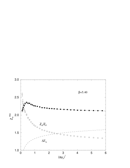
Figure 2: $\Delta Z_{m}^{\mbox{\tiny$R\!G\!I$}}$ (dashed line), $Z_{A}/Z_{P}^{\mbox{\tiny$R\!I\!\!-\!\!M\!O\!M$}}$ (empty squares) and $Z_{m}^{\mbox{\tiny$R\!G\!I$}}$ (filled circles) for $\beta=5.40$ (filled circles), together with a fit $F(a\mu_{p})=p_{1}+p_{2}(a\mu_{p})^{2}+p_{3}/(a\mu_{p})^{2}$.

we show $\Delta Z^{\mbox{\tiny$R\!I^{\prime}\!\!-\!\!M\!O\!M$}}_{m}$, $Z_{A}/Z_{P}^{\mbox{\tiny$R\!I^{\prime}\!\!-\!\!M\!O\!M$}}$ and their product, giving $Z_{m}^{\mbox{\tiny$R\!G\!I$}}$ for $\beta=5.40$. This should be independent of the scale $(a\mu_{p})^{2}$ at least for larger values. This seems to be the case, we make a phenomenological fit to account for residual $(a\mu_{p})^{2}$ effects.

With $Z_{m}^{\mbox{\tiny$R\!G\!I$}}$, we can now find $r_{0}m_{q}^{\mbox{\tiny$R\!G\!I$}}$ and hence the ratio $r_{0}m_{q}^{\mbox{\tiny$R\!G\!I$}}/(r_{0}m_{ps})^{2}$, using the values of $r_{0}/a$ given in [6]. In Fig. 3 we plot this ratio

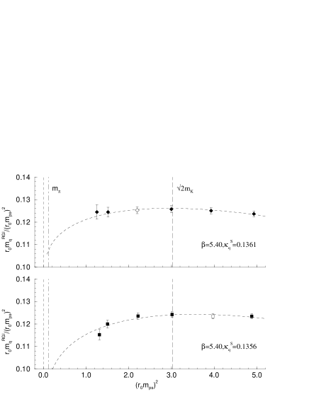
Figure 3: $r_{0}m_{q}^{\mbox{\tiny$R\!G\!I$}}/(r_{0}m_{ps})^{2}$ against $(r_{0}m_{ps})^{2}$, together with a fit using eq. (5) for $\beta=5.40$. Filled points represent valence quark results while unfilled points are the sea quark results. The dashed line (labelled ‘$\sqrt{2}m_{K}$’) represents a fictitious particle composed of two strange quarks, which at LO $\chi$PT is given from eq. (4) by $\sqrt{(r_{0}m_{K^{+}})^{2}+(r_{0}m_{K^{0}})^{2}-(r_{0}m_{\pi^{+}})^{2}}$, while the dashed-dotted line (labelled ‘$m_{\pi}$’) representing a pion with mass degenerate $u/d$ quark is given by $r_{0}m_{\pi^{+}}$.

(against $(r_{0}m_{ps})^{2}$) for $\beta=5.40$. Using eq. (4) to eliminate $c_{a}^{\mbox{\tiny$R\!G\!I$}}$ in favour of $r_{0}m_{s}^{\mbox{\tiny$R\!G\!I$}}/((r_{0}m_{K^{+}})^{2}+(r_{0}m_{K^{0}})^{2}-(r_{0}m_{\pi^{+}})^{2})$ in eq. (5) gives $r_{0}m_{s}^{\mbox{\tiny$R\!G\!I$}}$ directly to NLO in our fit function.

We have restricted the quark masses to lie in the range $(r_{0}m_{ps})^{2}<5$, which translates to $m_{ps}\mathrel{\hbox to0.0pt{\lower 4.0pt\hbox{\hskip 1.0pt$\sim$}\hss}\raise 1.0pt\hbox{$<$}}850\,\mbox{MeV}$, which is hopefully within the range of validity of low order $\chi$PT results. (Indeed using $r_{0}/a$, rather than their chirally extrapolated values for example, tends to give less variation in the ratio $r_{0}m_{q}^{\mbox{\tiny$R\!G\!I$}}/(r_{0}m_{ps})^{2}$ so we expect LO $\chi$PT to be markedly dominant.) Thus finally, for each $\beta$-value we have determined $r_{0}m_{s}^{\mbox{\tiny$R\!G\!I$}}$ and can now perform the last extrapolation to the continuum limit.

2 Results

Our derivation so far, although needing a secondary quantity such as $r_{0}/a$ for a unit, depends only on lattice quantities. Only at the last stage, with our direct fit did we need to give a physical scale to this unit. A popular choice is $r_{0}=0.5\,\mbox{fm}$. However there are some uncertainties in this value; our derivation using the nucleon gave $r_{0}=0.467\,\mbox{fm}$ and so to give some idea of scale uncertainties, we shall consider both values. (The main change when changing the scale comes from the $r_{0}$s in eq. (4), as $m^{\mbox{\tiny$R\!G\!I$}}_{s}\propto r_{0}$, while changes in $\Delta Z^{\mbox{\tiny$\overline{MS}$}}_{m}$ are only logarithmic.)

Using the results from section 1.1 for $[\Delta Z_{m}^{\mbox{\tiny$\overline{MS}$}}(2\,\mbox{GeV})]^{-1}$ to convert $m_{s}^{\mbox{\tiny$R\!G\!I$}}$ to $m_{s}^{\mbox{\tiny$\overline{MS}$}}(2\,\mbox{GeV})$ gives the results shown in Fig. 4. Also shown is an

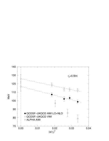
Figure 4: Results for $m_{s}^{\mbox{\tiny$\overline{MS}$}}(2\,\mbox{GeV})$ (filled circles) versus the chirally extrapolated values of $(a/r_{0})^{2}$ (as given in [6]) together with a linear extrapolations to the continuum limit. For comparison, we also give our previous result using the VWI, [9] (open squares) and the ALPHA AWI determination from [12], (open triangles).

extrapolation to continuum limit. We finally find the result

$$m_{s}^{\mbox{\tiny$\overline{MS}$}}(2\,\mbox{GeV}) = \left\{\begin{array}[]{lll}117(7)\,\mbox{MeV}&\mbox{for}&r_{0}=0.5\,\mbox{fm}\\ 111(6)\,\mbox{MeV}&\mbox{for}&r_{0}=0.467\,\mbox{fm}\\ \end{array}\right.\,,$$ (11)

where the error is statistical. This is to be compared to our previous result using the VWI, [9], which gave results of $126(5)\,\mbox{MeV}$, $119(5)\,\mbox{MeV}$ for $r_{0}=0.5\,\mbox{fm}$ and $0.467\,\mbox{fm}$ respectively. We take a further systematic error on these results as being covered by the different $r_{0}$ values of about $\sim 6\,\mbox{MeV}$. Although the continuum extrapolation should be treated with caution, it does indicate that the strange quark mass for 2-flavour QCD lies in the region of $100$ – $130\,\mbox{MeV}$.

References

[1]
M. Göckeler et al., in preparation.
[2]
T. van Ritbergen et al.,
Phys. Lett.B400 379 (1997)
[hep-ph/9701390].
[3]
J. A. M. Vermaseren et al.,
Phys. Lett.B405 327 (1997)
[hep-ph/9703284].
[4]
G. Martinelli et al.,
Nucl. Phys.B445 81 (1995)
[hep-lat/9411010].
[5]
K. G. Chetyrkin et al.,
Nucl. Phys.B583 3 (2000)
[hep-ph/9910332].
[6]
M. Göckeler et al.,
hep-ph/0502212.
[7]
C. Bernard et al.,
Phys. Rev.D49 486 (1994)
[hep-lat/9306005].
[8]
S. R. Sharpe,
Phys. Rev.D56 7052 (1997),
erratum ibid. D62 (2000) 099901
[hep-lat/9707018].
[9]
M. Göckeler et al.,
hep-ph/0409312.
[10]
M. Della Morte et al.,
JHEP0503 029 (2005)
[hep-lat/0503003].
[11]
J. R. Cudell et al.,
Phys. Lett.B454 105 (1999)
[hep-lat/9810058].
[12]
M. Della Morte et al.,
hep-lat/0507035.
[13]
C. R. Allton et al.,
Phys. Rev.D65 054502 (2002) [hep-lat/0107021].