Field Theory Simulations on a Fuzzy Sphere   —
an Alternative to the Lattice

Abstract:

We explore a new way to simulate quantum field theory, without introducing a spatial lattice. As a pilot study we apply this method to the 3d $\lambda\phi^{4}$ model. The regularisation consists of a fuzzy sphere with radius $R$ for the two spatial directions, plus a discrete Euclidean time. The fuzzy sphere approximates the algebra of functions of the sphere with a matrix algebra, and the scalar field is represented by a Hermitian $N\times N$ matrix at each time site. We evaluate the phase diagram, where we find a disordered phase and an ordered regime, which splits into phases of uniform and non-uniform order. We discuss the behaviour of the model in different limits of large $N$ and $R$, which lead to a commutative or to a non-commutative $\lambda\phi^{4}$ model in flat space.

PoS(LAT2005)263

1 The $\lambda\phi^{4}$ model on a fuzzy sphere

In this work we deal with the fuzzy sphere formulation as a method to discretise quantum field theory, and we apply it in numerical simulations of the 3d $\lambda\phi^{4}$ model. In that scheme, the regularisation of the spatial part of the action takes place in angular momentum space, rather than coordinate space, hence no space lattice is involved. Nevertheless we arrive at a finite set of degrees of freedom, which allows us to study the model non-perturbatively.

In particular we are going to regularise the continuum action

$$S(\phi) = \int_{S^{1}}dt\ s(\phi,t)\ ,$$

$$s(\phi,t) = \int_{S^{2}}\left[\frac{1}{2}\phi(t,x)\left(\frac{{\mathcal{L}}^{2}}{R^{2}}-\partial_{t}^{2}\right)\phi(t,x)+\frac{m^{2}}{2}\phi^{2}(t,x)+\frac{\lambda}{4}\phi^{4}(t,x)\right]R^{2}d\Omega\ ,$$ (1)

where $d\Omega=\sin\theta d\theta d\phi$, and $S_{1}$ has circumference $T$. The scalar field $\phi(t,x)$ depends on the Euclidean time $t$ and the space coordinates $x_{i}(\theta,\phi)$, with the constraint $\sum_{i=1}^{3}x_{i}^{2}=R^{2}$. ${\mathcal{L}}_{i}$ are the angular momentum operators, and ${\mathcal{L}}^{2}=\sum_{i=1}^{3}{\mathcal{L}}_{i}^{2}$.

We first focus on $s(\phi,t)$, the spatial part of this action. As a discretisation we replace $S^{2}$ by a fuzzy sphere [3]: this means that the coordinates $x_{i}$ are replaced by the coordinate operators $X_{i}=\frac{2R}{\sqrt{N^{2}-1}}L_{i}$  ($i=1,2,3$), where $L_{i}$ are the $SU(2)$ generators in the $N$-dimensional irreducible representation. These coordinate operators satisfy the constraint $\sum_{i=1}^{3}X_{i}^{2}=R^{2}\cdot 1\!\!\!1\$, which corresponds to a matrix equation for a sphere. The $X_{i}$ obey the commutation relation

$$\left[X_{i},X_{j}\right]=i\epsilon_{ijk}\frac{2R}{\sqrt{N^{2}-1}}X_{k}\ .$$ (2)

At finite $N$ our coordinates describes a non-commutative geometry; the sphere turns fuzzy.

As in the continuum, where $\phi$ can usually be expressed as a polynomial in the coordinates $x_{i}$, its fuzzy counterpart $\Phi$ can be written as a polynomial in the coordinate operators. This formulation is obtained by replacing $C^{\infty}(S^{2})$, the algebra of smooth functions on the sphere, by ${\tt Mat}_{N}$, a sequence of matrix algebras of dimension $N$, where all positive integer values of $N$ are permitted [4]. Thus the scalar field is represented by a Hermitian matrix $\Phi$ of dimension $N$ (note that $\phi\in\mathbb{R}$ implies the Hermiticity of the matrix $\Phi$).

The differential operators ${\cal L}_{i}\,\cdot$ are replaced by $\left[L_{i},\cdot\,\right]$, and the integral over $S^{2}$ is converted to the trace. The standard basis for functions on the sphere — given by the spherical harmonics $\{Y_{lm}\}$ — is replaced by the polarisation tensor basis $\{\hat{Y}_{lm}\}$, see for instance Ref. [5]. Let us summarise this set of substitutions:

$$x_{i}\in C^{\infty}(S^{2})\ \longrightarrow\ X_{i}\in{\tt Mat}_{N} \quad\phi(x)\in C^{\infty}(S^{2})\ \longrightarrow\ \Phi\in{\tt Mat}_{N}\ ,$$ , (3)

$${\cal L}_{i}\phi(x)\ \longrightarrow\ \left[L_{i},\Phi\right] \quad{\cal L}^{2}\cdot\longrightarrow\hat{\cal L}^{2}\cdot:=\sum_{i=1}^{3}\left[L_{i},\left[L_{i},\cdot\right]\right]\ ,$$ , (4)

$$\int_{S^{2}}\phi(x)d\Omega \longrightarrow \frac{4\pi}{N}{\rm Tr}\left(\Phi\right)\ .$$ (5)

Rotations on the fuzzy sphere are performed by using an element $U$ of the $N$ dimensional unitary irreducible representation of $SU(2)$. A general element $U$ of this representation has the form $U=\exp(i\omega_{i}L_{i})$, with $\omega_{i}\in\mathbb{R}$. The coordinate operators are then rotated as $UX_{i}U^{\dagger}={\mathtt{R}}_{ij}X_{j}\,,\ \mathtt{R}\in SO(3)$, and the field transforms as $\Phi\longrightarrow\Phi^{\prime}=U\Phi U^{\dagger}$.

Implementing the substitutions (3)-(5) in the action (1), we obtain

$$s(\Phi(t))=\frac{4\pi R^{2}}{N}{\rm Tr}\Big{[}\frac{1}{2}\Phi(t)\left(\frac{\hat{\cal L}^{2}}{R^{2}}-\partial_{t}^{2}\right)\Phi(t)+\frac{m^{2}}{2}\Phi^{2}(t)+\frac{\lambda}{4}\Phi^{4}(t)\Big{]}\ .$$ (6)

This discretisation (at finite $N$) preserves the exact rotational symmetry of the continuum model, since any rotation on the sphere is allowed, and action (6) remains invariant.

To discretise the time direction we take a set of $N_{{t}}$ equidistant points, $T=N_{{t}}\Delta t$, with periodic boundary conditions. This yields the fully regularised action

$$S\left[\Phi\right]=\frac{4\pi R^{2}\Delta t}{N}\sum_{{t}=1}^{N_{{t}}}{\rm Tr}\Big{[}\frac{1}{2R^{2}}\Phi\left(t\right)\hat{\cal L}^{2}\Phi\left(t\right)+\frac{1}{2}\left(\frac{\Phi(t+\Delta t)-\Phi(t)}{\Delta t}\right)^{2}+\frac{m^{2}}{2}\Phi^{2}(t)+\frac{\lambda}{4}\Phi^{4}(t)\Big{]}\ .$$ (7)

We are interested in the limits $N\longrightarrow\infty$ and $N_{{t}}\longrightarrow\infty$, and for our simulations we fixed $N=N_{{t}}$. One configuration $\Phi$ corresponds to a set of matrices $\{\Phi(t)\}$, for ${t}=\Delta t,\dots,N_{t}\Delta t$.

The formal expression for the Fourier decomposition of the field reads

$$\Phi(t)=\sum_{l=0}^{\infty}\ \sum_{m=-l}^{l}\ \sum_{k\in Z\!\!\!Z}\,c_{lm}(k)\,\exp\left(i\frac{2\pi kt}{N_{{t}}}\right)\,\hat{Y}_{lm}\ ,\quad c_{lm}(k)=\frac{4\pi R^{2}}{NN_{t}}\sum_{t}\exp(-i\frac{2\pi kt}{N_{t}}){\rm Tr}(\hat{Y}_{lm}^{{\dagger}}\Phi(t))$$ (8)

In particular the temporal zero mode of $\Phi$ is given by

$$\bar{\Phi}=\frac{1}{N_{{t}}}\sum_{{t}=1}^{N_{{t}}}\Phi(t)=\mathbf{c}_{00}\hat{Y}_{00}+\sum_{m=-1}^{1}\mathbf{c}_{1m}\hat{Y}_{1m}+\dots$$ (9)

where $\mathbf{c}_{lm}:=\frac{1}{N_{{t}}}\sum_{{t}}c_{lm}({t}).$ Our order parameters are based on the coefficients $\mathbf{c}_{lm}$,

$$\varphi_{0}:=|\mathbf{c}_{00}|\ ,\qquad\varphi_{1}:=\sqrt{\sum_{m=-1}^{1}|c_{1,m}{|}^{2}}\ ,$$ (10)

and the corresponding susceptibilities. We define $\varphi_{all}^{2}$ as the norm of the field $\bar{\Phi}$,

$$\varphi_{all}^{2}:=\sum_{l,m}|\mathbf{c}_{lm}|^{2}=\frac{4\pi}{N}{\rm Tr}\left(\bar{\Phi}^{2}\right)=\varphi_{0}^{2}+\varphi_{1}^{2}+\dots$$ (11)

2 Numerical results

A numerical study of the 2d version of this model was presented in Ref. [6]. However, as an important qualitative difference, in that case the radius $R$ could be absorbed in the couplings, whereas here it takes the rôle of an independent parameter.

We also recall that our formulation corresponds to a non-commutative space on the regularised level. In analogy to previous studies of the non-commutative $\lambda\phi^{4}$ model in flat spaces [7], and to the 2d $\lambda\phi^{4}$ on a fuzzy sphere [6], we observed three phases:

• I : The disordered phase, characterised by $\varphi_{all}^{2}\approx 0$, $\varphi_{0}\approx 0$, $\varphi_{1}\approx 0,\ \dots$

• II : The uniform order, characterised by $\varphi_{all}^{2}\approx\varphi_{0}^{2}>0$, $\varphi_{1}\approx 0$, $\dots$

• III : The non-uniform order, e.g. $\varphi_{all}^{2}>0$, $\varphi_{0}\approx 0$; $\varphi_{1}>0$, $\varphi_{2}\approx 0,\ \dots$

Figures 1 to 3 give an overview of our numerical results.

The triple point $\left(\lambda_{T},m^{2}_{T}\right)$ is fixed by the intersection of the transition curves $I-II$ and $I-III$. We focus on its behaviour since it determines which phases survive under different limits. The emerging triple point expression reads

$$\left(\Delta t\lambda_{T},\Delta t^{2}m^{2}_{T}\right)=\left((41.91\pm 30)\left(\frac{\Delta t^{2}}{NR^{2}}\right)^{\gamma},-(12.7\pm 1)\left(\frac{\Delta t}{R}\right)^{3\gamma^{\prime}}\right)\ ,$$ (12)

where our numerical results are consistent with $\gamma=\gamma^{\prime}=0.64\pm 0.2$.

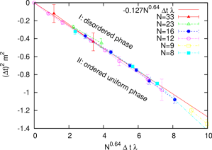
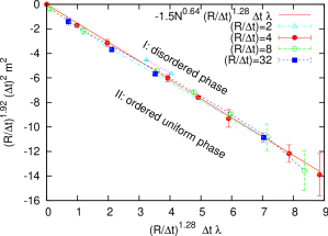
Figure 1: Examples for the phase transition curves I-II: On the left we fix $\frac{R}{\Delta t}=4$ and vary $N$. On the right we fix $N=12$ and and vary the ratio $\frac{R}{\Delta t}$. In both cases the transition lines stabilise for suitably scaled axes.

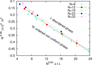
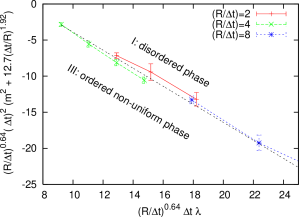
Figure 2: Examples for the phase transition curves I-III: On the left we fix $\frac{R}{\Delta t}=8$ and vary $N$. On the right we fix $N=16$ and and vary the ratio $\frac{R}{\Delta t}$. Also here the transition lines stabilise for suitably scaled axes.

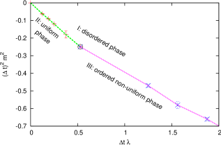
Figure 3: The phase diagram for $N=16$, $\frac{R}{\Delta t}=4$. We show linear fits for both transition curves. The extrapolation of those lines allow us to identify the triple point.

3 Behaviour of the model under different limits

For the temporal part of the model we set $\Delta t=\frac{1}{N^{\kappa}}$, $\kappa\in(0,1)$, hence the time extent $T$ amounts to $N^{1-\kappa}\longrightarrow\infty$.

• Regarding the spatial part of the model, the non-commutative Moyal plane limit $\mathbb{R}_{\Theta}^{2}$ can be accessed if $R^{2}=\frac{N\Theta}{2}$, for $\Theta$ fixed and $R,\,N\longrightarrow\infty$  [8].

• For the commutative flat limit, $\mathbb{R}^{2}$, we take $R\propto N^{\frac{1}{2}(1-\epsilon)}$ with $\epsilon\in(0,1)$, and $N\longrightarrow\infty$.

• The commutative sphere limit arises when $R$ is fixed and $N\longrightarrow\infty$, since $C^{\infty}(S^{2})$ is recovered.

We summarise all cases by setting $R=N^{\beta}$ with $\beta=\frac{1}{2}(1-\epsilon)$, $\epsilon\in[0,1]$. Then eq. (12) takes the form

$$\left(\lambda_{T},m^{2}_{T}\right)=\left(41.91N^{\kappa(1-2\gamma)-\gamma(1+2\beta)},-12.7N^{2\kappa-3\gamma^{\prime}(\beta+\kappa)}\right)\ .$$ (13)

Although the error on $\gamma$ resp. $\gamma^{\prime}$ is sizable, the exponent in $\lambda_{T}$ in eq. (13) seems to be clearly negative. Therefore $\lambda_{T}\longrightarrow 0$ as $N\longrightarrow\infty$, which indicates the disappearance of the uniform order phase.

As a particular case we consider $\kappa=\frac{1}{2}$, with the tri-critical action

$$S_{T}(\Phi) \approx \sum_{{t}=1}^{N}{\rm Tr}\Big{[}\frac{2\pi}{N}\Phi\left(t\right)\hat{\cal L}^{2}\Phi\left(t\right)+2\pi N^{2\beta}\left[\Phi(t+\Delta t)-\Phi(t)\right]$$ (14)

$$\qquad-\frac{25.4\pi}{N}\Phi^{2}(t)+\frac{41.9\pi}{N}N^{\gamma(\beta-\frac{1}{2})}\Phi^{4}(t)\Big{]}\ .$$

For large $N$ the leading contribution to eq. (14) is the temporal kinetic term, while the contribution from the fuzzy kinetic term is negligible. Hence the uniform order phase disappears in this limit, which leads to a simplified model that was analysed in Refs. [9].

Finally we compare our results to those obtained in the last work quoted in Ref. [7]. If we set $\Delta t=1$ and $R=N$, we arrive at a similar behaviour of the triple point, namely $\left(N^{2}\lambda_{T},N^{2}m^{2}_{T}\right)\approx const$. The suitable action is given by eq. (14) at $\beta=1/2$. Again the leading contribution is due to the temporal kinetic term.

4 Conclusions

We presented a numerical study of the $\lambda\Phi^{4}$ model on the 3 dimensional Euclidean space where we combined two schemes of discretisation. As in related models studied previously [6, 7], we identified the existence of three phases, one of which is unknown in the $\lambda\phi^{4}$ model in the continuous commutative space. The fate of these phases under various limits will be discussed in more detail in Ref. [10].

At this point, we just repeat that the triple point scales to zero in the limit $N\rightarrow\infty$. Hence this simple model cannot capture the Ising universality class in this limit. This is not surprising, given the perturbative results of Refs. [4] and [8], where it was observed (in the commutative limit) that though the non-planar diagrams have the same divergence at $N\rightarrow\infty$ as the planar diagrams, the difference of the two diagrams is finite and non-local.

In any case, to maintain the uniform phase, it is necessary to reinforce the fuzzy kinetic term. This is achieved most simply by adding a higher derivative contribution which will guarantee that all diagrams are convergent in the large $N$ limit. For the current model this would correspond to adding a term $\Phi(\hat{\cal L}^{2})^{2}\Phi/(\Lambda^{2}R^{4})$ inside the trace in eq. (7) (where $\Lambda$ is a momentum cutoff). By an appropriate scaling of $\Lambda$ it should be possible to send the triple point to infinity as $N\rightarrow\infty$.

This pilot study reveals that the fuzzy sphere formulation does indeed enable numerical simulations without the requirement of a spatial lattice. Its virtue as a discretisation scheme is that it preserves certain symmetries exactly, which are explicitly broken on the lattice. We hope for that virtue to become powerful in particular in supersymmetric models.

Acknowledgements   We are indebted to A. Balachandran, B. Dolan, X. Martin, J. Nishimura, M. Panero, P. Prešnajder, H. Steinacker, J. Volkholz and B. Ydri for inspiring discussions. This work was supported in part by the “Deutsche Forschungsgemeinschaft” (DFG).

References

- [1]
- [2]
- [3] J. Hoppe, Ph.D. Thesis MIT (Cambrdige MA, 1982), Elem. Part. Res. J. (Koyoto) 80 (1989 145. J. Madore, Class. and Quant. Grav. ~ (9) (1992) 69. H. Grosse, C. Klimčík and P. Prešnajder, Int. J. Theor. Phys. ~ (35) (1996) 231 [hep-th/9505175], Commun. Math. Phys. ~ (180) (1996) 429 [hep-th/9602115]. S. Baez, A.P. Balachandran, S. Vaidya and B. Ydri, Commun. Math. Phys. ~ (208) (2000) 787 [hep-th/9811169]. A.P. Balachandran, X. Martin and D. O’Connor, Int. J. Mod. Phys. A ~ (16) (2001) 2577 [hep-th/0007030]. B. Ydri, Ph. D. thesis, Syracuse University (Syracuse N.Y., 2001) [hep-th/0110006].
- [4] R. Delgadillo, Master Thesis, CINVESTAV (Mexico D.F., 2002). B.P. Dolan, D. O’Connor and P. Prešnajder, J. High Energy Phys. ~ (03) (2002) 013 [hep-th/0109084]. H. Steinacker, JHEP 0503 (2005) 075 [hep-th/0501174].
- [5] D.A. Varshalovich, A.N. Moskalev and V.K. Khersonky, Quantum Theory of Angular Momentum: Irreducible Tensors, Spherical Harmonics, Vector Coupling Coefficients, 3nj Symbols, World Scientific, Singapore (1998).
- [6] X. Martin, JHEP 0404 (2004) 077 [hep-th/0402230].
- [7] S.S. Gubser and S.L. Sondhi, Nucl. Phys. B 605 (2001) 395 [hep-th/0006119]. G.-H. Chen and Y.-S. Wu, Nucl. Phys. B 622 (2002) 189 [hep-th/0110134]. J. Ambjørn and S. Catterall, Phys. Lett. B 549 (2002) 253 [hep-lat/0209106]. P. Castorina and D. Zappalà, Phys. Rev. D 68 (2003) 065008 [hep-th/0303030]. F. Hofheinz, Ph.D. Thesis (Berlin, 2003) [hep-th/0403117]. W. Bietenholz, F. Hofheinz and J. Nishimura, Fortsch. Phys. 51 (2003) 745 [hep-th/0212258], Acta Phys. Polon. B 34 (2003) 4711 [hep-th/0309216], JHEP 0406 (2004) 042 [hep-th/0404020].
- [8] C.-S. Chu, J. Madore and H. Steinacker, JHEP 0108 (2001) 038 [hep-th/0106205].
- [9] A. Matytsin, Nucl. Phys. B 411 (1994) 805 [hep-th/9306077]. B. Eynard, J. Phys. A 31 (1998) 8081 [cond-mat/9801075]; JHEP 0301 (2003) 051 [hep-th/0210047].
- [10] W. Bietenholz, F. Hofheinz, J. Medina and D. O’Connor, in preparation.