Searching for the critical endpoint in QCD with two quark flavors

Abstract:

I present a method which can be used to locate the expected critical endpoint of the phase diagram of QCD with two light quark flavors. I illustrate the ideas on a suitable Random Matrix Model and show preliminary results in QCD

PoS(LAT2005)161

1 The expected phase diagram of QCD

It is belived that the phase diagram of QCD is very rich, especially at low temperatures, where many different phases separated by phase boundaries are expected. The analysis which lead to these expectations are based on symmetries, effective theories, models, and analogies, and therefore are far from being well established [1].

The major problem in the study of the QCD phase diagram is that standard Monte Carlo simulations cannot be used in QCD with baryon chemical potential since the fermion determinant is complex and cannot be included in a probability measure. It is the so called sign problem. But even at zero chemical potential the situation is not clear: in QCD with two degenerate light quarks the nature of the deconfinement transition at finite temperature is not definitely established, and it is not even clear whether it is a crossover or a true phase transition, either of first or second order class [2]. Until recently, it has been generally accepted that it is a crossover, in which case the change from the confinement to the deconfinement regime at high temperature and low baryon chemical potential would also be a crossover. Since a first order deconfinement transition is expected at sufficiently low temperatures, there must be a critical point located where the first order transition ceases to exist and is replaced by a crossover. This is the critical endpoint. The expected phase diagram is depicted in Figure 1. A Chiral Random Matrix Model predicts this phase structure [3]. Lattice computations overcoming the sign problem by means of the double reweighting technique have found signals of a critical point [4].

In the following we will propose a method to locate the critical endpoint and present some preliminary results. We assume that at zero chemical potential the confinement and deconfinement regimes are separated by a crossover.

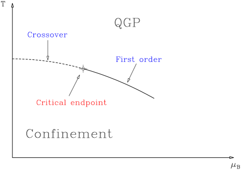
Figure 1: The expected phase diagram of two flavor QCD

2 The method

Let us describe the general setting. A more complete discussion can be found elsewhere [5]. We work on a lattice with a generalized staggered fermion action

$$S=\frac{1}{2}\sum_{n}\sum^{3}_{i=1}\bar{\psi}_{n}\eta_{i}(n)\left(U_{n,i}\psi_{n+i}-U^{\dagger}_{n-i,i}\psi_{n-i}\right)+m\sum_{n}\bar{\psi}_{n}\psi_{n}+S_{\tau}\,,$$ (1)

where $S_{\tau}$ contains the temporal (covariant) derivative, and therefore the temporal links:

$$S_{\tau}\;=\;\frac{x}{2}\sum_{n}\bar{\psi}_{n}\eta_{0}(n)\left(U_{n,0}\psi_{n+0}-U^{\dagger}_{n-0,0}\psi_{n-0}\right)\;+\;\frac{y}{2}\sum_{n}\bar{\psi}_{n}\eta_{0}(n)\left(U_{n,0}\psi_{n+0}+U^{\dagger}_{n-0,0}\psi_{n-0}\right)\,.$$ (2)

We consider $x$ and $y$ as independent parameters. QCD is recovered by setting $x=\cosh\mu$ and $y=\sinh\mu$, where $\mu$ is the baryon chemical potential. The sign problem is present if $\mathrm{Re}\,y\neq 0$. However, it is easy to see that there is no sign problem if $y$ is purely imaginary, $y=\mathrm{i}\bar{y}$, with $\bar{y}$ real. Imaginary chemical potential corresponds to $x=\cos\mu$ and $y=\mathrm{i}\sin\mu$.

It can be seen that the partition function (and therefore the phase diagram) depends on $x$ and $y$ only through the following two variables:

$$u\;=\;x^{2}-y^{2}\,,\hskip 28.45274ptv\;=\;(x+y)^{3L_{t}}+(x-y)^{3L_{t}}\,,$$ (3)

where $L_{t}$ is the lattice size in the temporal direction. This two variables are real for both real and imaginary $y$. Also, they are invariant under the change $y\rightarrow-y$ (or $\bar{y}\rightarrow-\bar{y}$) and $x\rightarrow-x$ separately, since $L_{t}$ is even. Altogether, this implies that the phase diagram can be plotted in the $(x^{2},y^{2})$ plane. Obviously, the semiplane $y^{2}<0$ corresponds to imaginary $y$. The physical region is the line $x^{2}-y^{2}=1$, with $x^{2}\geq 1$. Imaginary chemical potential corresponds to the line $x^{2}-y^{2}=1$, with $0\leq x^{2}\leq 1$. Numerical simulations are feasible for $x^{2}\geq 0$ and $y^{2}\leq 0$.

The expected phase diagram projected onto the $(x^{2},y^{2})$ plane is displayed in Figure 2. The extended phase diagram is three dimensional, with the temperature axis, which is not displayed, perpendicular to the $x^{2}$ and $y^{2}$ axis. We assume that on the physical line (the black line on the figure, made up of solid and dashed pieces), for large $x$ (i.e, large chemical potential) there is a first order phase transition (solid line), which ends at the critical endpoint, marked with an open symbol on the figure. For lower $x$ on the physical line there is a crossover (dashed line) separating the low temperature confining regime from the high temperature deconfined phase. The first order line is extended over a surface in the three dimensional phase diagram, and the critical point is extended along a line of critical points (blue line) which is the boundary of the first order surface (projected onto the $(x^{2},y^{2})$ plane on the figure).

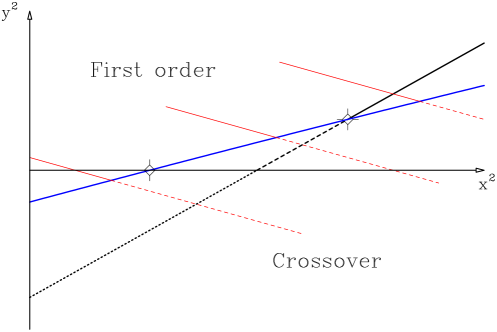
Figure 2: The expected phase diagram projected onto the $(x^{2},y^{2})$ plane. Although the transition lines are plotted as straight lines for simplicity, it should not be inferred we expect they have such simple form.

The $y^{2}=0$ axis is interesting because numerical simulations are feasible there. At $x=1$ and $y=0$, which is the zero chemical potential point on the physical line, there is a crossover, by assumption. On the other hand, at $x=0$ and $y=0$ the fermion determinant contains no temporal link –it contains only the spatial links– and obviously cannot break the Polyakov symmetry explicitely. Hence, the Polyakov loop is an order parameter. We expect center symmetry spontaneously broken at high temperature and a first order transition separating the low and high temperature phases. First order transitions are generically robust under perturbations and therefore there must be a first order transition for $y^{2}=0$ and any $x^{2}$ sufficiently small. This first order line must end at a critical point located at $x^{2}<1$ (marked with an open symbol on the figure), since we assume a crossover at $x^{2}=1$. The natural scenario is a critical line crossing the physical line at the physical critical endpoint and the $y^{2}=0$ axis at some point of the segment $0<x^{2}<1$, as the blue line of Figure 2.

The critical line can be determined for $y^{2}\leq 0$ by means of standard Monte Carlo simulations and extended to small positive $y^{2}$ by double reweighting. The resulting line might be extrapolated to the physical line and then the position of the physical critical endpoint would have been determined. Even if the extrapolation were not reliable, finding a critical line directed towards the physical line would be very interesting, since it would indicate the existence of the critical endpoint.

3 A Chiral Random Matrix Model

A Chiral Random Matrix Model of QCD predics the existence of a critical endpoint in the $(\mu,T)$ plane for light quarks [3]. We can adapt this model to study the structure of the extended phase diagram, in the $(x^{2},y^{2},T)$ space. To this end, let us consider the following partition function

$$\mathcal{Z}=\int[dA^{\dagger}dA][d\bar{\psi}_{L}d\psi_{L}d\bar{\psi}_{R}d\psi_{R}]\exp\left(-S\right)\,,$$ (4)

with

$$S=N\sum_{t=0}^{L_{t}-1}\mathrm{Tr}(A^{\dagger}_{t}A_{t})-\sum_{t=0}^{L_{t}-1}\left[\bar{\psi}^{a}_{L}(t)\mathrm{i}A_{t}\psi^{a}_{L}(t)+\bar{\psi}^{a}_{R}(t)\mathrm{i}A^{\dagger}_{t}\psi^{a}_{R}(t)\right]-m\sum_{t=0}^{L_{t}-1}\left[\bar{\psi}^{a}_{L}(t)\psi^{a}_{R}(t)+\bar{\psi}^{a}_{R}(t)\psi^{a}_{L}(t)\right]$$

$$-\beta\frac{x+y}{2}\sum_{t=0}^{L_{t}-1}\left[\bar{\psi}^{a}_{L}(t)\psi^{a}_{L}(t+1)+\bar{\psi}^{a}_{R}(t)\psi^{a}_{R}(t+1)\right]-\beta\frac{x-y}{2}\sum_{t=0}^{L_{t}-1}\left[\bar{\psi}^{a}_{L}(t+1)\psi^{a}_{L}(t)+\bar{\psi}^{a}_{R}(t+1)\psi^{a}_{R}(t)\right]\,,$$

where $A_{t}$ is a complex $N\times N$ random matrix depending on the temporal index $t$ ($N$ collects the color, Dirac, and spatial indices), $\psi^{a}_{L}(t)$ and $\psi^{a}_{R}(t)$ are respectively the left and right handed components of a fermion field, and $a$ is a flavor index. The parameter $m$ is the fermion mass, which will be set to zero in the following, $x$ and $y$ are the parameters introduced in the previous section, and $\beta$ controls the temperature (large $\beta$ corresponds to high temperature). Notice that, in order to introduce the chemical potential in the lattice way, we keep the dynamics local (and free for simplicity) in the temporal direction.

The model can be solved analytically in the large $N$ limit with the standard techniques. Figure 3 (left panel) displays the physical phase diagram ($x=\cosh\mu$, $y=\sinh\mu$) for $N_{t}=4$. There are two phases: at low temperature chiral symmetry is spontaneously broken and it is restored at high temperatures. The transition is second order at small $\mu$ and first order at large $\mu$. The separation between both lines is a tricritical point. With a small mass, the second order line becomes a crossover, the first order transition remains and the tricritical point becomes the critical endpoint. The phase diagram mimics perfectly what is expected in QCD. Its extension to the $(x^{2},y^{2})$ plane, displayed on the right panel of Figure 3, complies with our expectations: the black line is the physical line, the solid and dashed red lines are respectively first and second order transitions, and the blue line is the tricritical line, which in this case happens to be straight. It crosses the $y^{2}=0$ axis at $x^{2}=y^{2}=0$. This is a pathology of the model which can be easily understood. Moreover, the $(x^{2}=0,y^{2}=0)$ point is singular and the tricritical line could not be continued from it by, say, double reweighting. Notice however that this model is based only on chiral symmetry and does not incorporate the dynamics of the Polyakov loop, which is the basis of the argument of the previous section. Hence, it is interesting that its extended phase diagram showed the features we predicted.

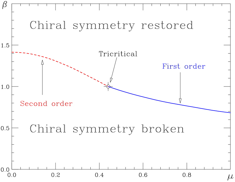
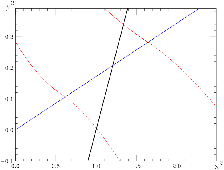
Figure 3: The physical phase diagram of the CRMM (left) and its extension to the $(x^{2},y^{2})$ plane (right).

4 Preliminary results for QCD

Figure 4 displays histograms of the modulus of the Polyakov loop from simulations of QCD performed with the R-algorithm. Since it has been pointed out that the systematics of this algorithm lead to wrong results for the time steps which use to be used [6], the results should be taken with some caution (the extrapolation to zero time step should be addressed before extracting any conclusion). Anyway, they are very preliminary. We take two flavors of staggered quarks, with mass $ma=0.05$, and explore the $y=0$ axis on lattices of temporal extent $L_{t}=4$ and spatial extent $L_{s}=6,8,10$. For each $x$ the value of the gauge coupling, $\beta$, has been tuned to its “critical” value.

For $x=0$ we see a kind of (not very clear) double pick structure on the $L_{s}=6$ lattice, wich becomes clearer as $L_{s}$ increases. The data point out to a first order transition (remenber the action has exact Polyakov symmetry in this case). The situation for $x=0.5$ is similar. For $x=0.7$, however, it is the opposite. We see a clear two pick structure on the $L_{s}=6$ lattice which is disappearing as $L_{s}$ increases, signaling a crossover. There must be a critical point between $x=0.5$ and $x=0.7$. Locating it accurately is a hard task which is in progress.

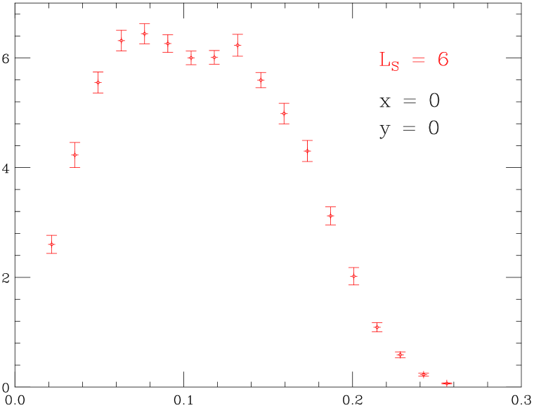
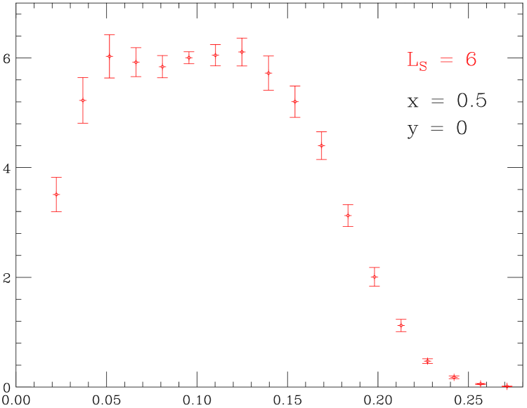
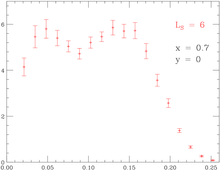
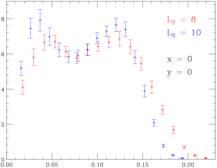
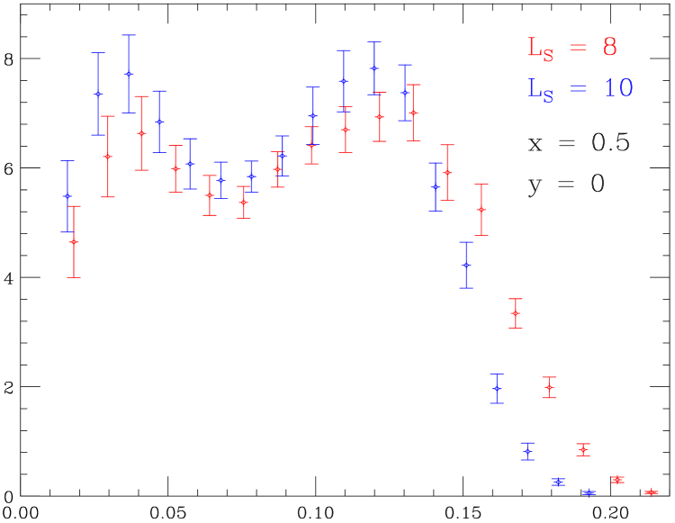
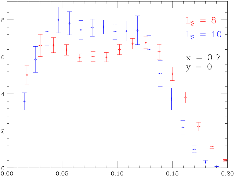
Figure 4: Histograms of the modulus of the Polyakov loop in two flavor QCD.

References

- [1] J.B. Kogut and M. Stephanov The phases of Quantum Chromodynamics, Cambridge University Press, Cambridge (UK) 2004.
- [2] M. D’Elia, A. Di Giacomo, and C. Pica, hep-lat/0503030.
- [3] M.A. Halasz, A.D. Jackson, R.E. Shrock, M.A. Stephanov, and J.J.M. Verbaarschot, Phys. Rev. D 58 (1998) 096007 [hep-ph/9804290].
- [4] Z. Fodor and S.D. Katz, JHEP 03 (2002) 014 [hep-lat/0106002]; JHEP 04 (2004) 050 [hep-lat/0402006].
- [5] V. Azcoiti, G. Di Carlo, A. Galante, and V. Laliena, JHEP 12 (2004) 010 [hep-lat/0409157]; Nucl. Phys. B 723 (2005) 77 [hep-lat/0503010].
- [6] J.B. Kogut and D. Sinclair, hep-lat/0504003; hep-lat/0509095.