Lattice QCD with light Wilson quarks

Abstract:

Wilson’s formulation of lattice QCD is attractive for many reasons, but perhaps mainly because of its simplicity and conceptual clarity. Numerical simulations of the Wilson theory (and of its improved versions) tend to be extremely demanding, however, to the extent that they rapidly become impractical at small quark masses. Recent advances in simulation algorithms now allow such simulations to be pushed to significantly smaller masses without having to compromise in other ways. Contact with chiral perturbation theory can thus be made and many physics questions can be addressed that previously appeared to be inaccessible.

PoS(LAT2005)002

1 Introduction

Several formulations of lattice QCD are currently in use, all having various advantages and shortcomings. There are good reasons, however, to proceed with the one proposed by Wilson long ago [1]. In particular, this formulation respects basic principles such as locality and unitarity, and it also preserves most symmetries of the continuum theory exactly. The axial chiral symmetries are among those that are not preserved, but it was understood in the 90’s that the chiral-symmetry violations can be reduced to small corrections of order $a^{2}$ (at lattice spacings $a\leq 0.1\,{\rm fm}$) by adding O($a$) counterterms to the lattice action and the composite gauge-invariant fields of interest [2, 3]. Non-perturbative renormalization techniques were then developed, and many physical quantities were calculated in the quenched (or valence) approximation, using numerical simulations.

When the sea-quark effects are included in the simulations, much more computer time is required, particularly so in the chiral regime of QCD, where the widely used simulation algorithms slow down proportionally to the second or maybe even the third power of the masses of the light quarks [4]–[15]. So far, simulations of the Wilson theory (with or without O($a$) corrections) thus proved to be impractical at lattice spacings $a\leq 0.1\,{\rm fm}$ and light-quark masses significantly smaller than half the physical mass of the strange quark.

2 Recent advances in simulation algorithms

Eventually many different lattices will have to be simulated, with lattice spacings as small as $0.04$ fm perhaps, and spatial sizes from, say, $2$ to $5$ fm. Moreover, the light-quark masses on these lattices should be such that the physical point can be reached with at most a short extrapolation. Taken together, these requirements imply large lattices, of size $48\times 24^{3},64\times 32^{3}$ and $96\times 48^{3}$ for example, and a situation, where the numerical solution of the lattice Dirac equation for a single source field requires as much as $10^{3}$–$10^{4}$ applications of the Dirac operator.

While the available computers become more powerful at an exponential rate, it is quite clear that better algorithms will be needed as well if these simulations are to be performed in the next few years. There are in fact new opportunities for algorithmic improvements once very large lattices are considered. The separation of short- and long-distance effects along the lines proposed by Peardon and Sexton [16], for example, is potentially more profitable if the lattice covers a wide range of scales.

The last few years have seen several developments that go in this general direction, one of them being the introduction of domain-decomposition methods in lattice QCD [17]. This led to a fast parallel solver for the lattice Dirac equation [18] and to an efficient simulation algorithm for two-flavour QCD (with mass-degenerate quarks), which scales well with the lattice size and the quark mass [19].

Progress has also been made using the Hybrid-Monte-Carlo (HMC) algorithm [20] with even–odd preconditioning and two pseudo-fermion fields, as suggested some time ago by Hasenbusch [21]. Early studies of this algorithm reported speed-up factors of $2$ or so with respect to the case where only one pseudo-fermion field is used [22, 23], but according to a recent paper by Urbach et al. [24], more impressive acceleration factors can be achieved at small quark masses if the parameters of the algorithm are properly tuned.

In this talk, however, the focus will be on the new simulation algorithm mentioned above, which is based on a domain decomposition of the lattice. The general strategies are first discussed, then the algorithm itself, and finally some simulation results [25] that have been obtained with it.

3 Domain-decomposition methods

Probably the first domain-decomposition method goes back to Hermann Amandus Schwarz, a well-known mathematician of the 19th century. One of the questions Schwarz posed himself was whether it is possible to solve the Dirichlet problem in complicated domains (the union of a disk and a square for example) in a constructive way. He then showed that the solution can be obtained through a convergent iteration, in which the Laplace equation is solved alternately in overlapping sub-domains, with boundary values given by the current approximate solution in the full domain. This ingenious method is now referred to as the Schwarz alternating procedure and is widely used, in the form of a preconditioner, for the numerical solution of elliptic partial differential equations (see ref. [26] for an introduction and a list of references).

There are at least three reasons for the popularity of domain-decomposition methods:

Parallel efficiency. Domain decompositions often map to the nodes of a parallel computer in a natural way. Using specially designed algorithms that spend most of the time on the sub-domains, it is then possible to reduce the communication overhead significantly. While this is a purely technical point, the parallel efficiency of an algorithm is an all-important issue in practice, when large systems are considered.

Mode separation. In many cases the dynamics of the low- and high-frequency modes of the system is very different so that it may be advisable to treat these modes separately. The division of space into sub-domains divides the modes into local and global ones, thus providing an obvious opportunity to implement the mode separation.

Scaling behaviour. Good algorithms should scale slowly with the parameters of the physical system. An almost complete elimination of the so-called critical slowing down is rare, but it is quite common that domain-decomposition methods achieve an improved scaling behaviour, particularly so when combined with multigrid ideas or other sophisticated techniques.

All these points are also relevant here, although there are important differences with respect to the well-known cases where domain-decomposition methods are used. In particular, the stochastic nature of the gauge field variables in lattice QCD excludes a straightforward application of multigrid methods.

4 Algorithmic strategies for QCD

The domain decompositions that will be considered in the following are divisions of the lattice into non-overlapping rectangular blocks such as the one shown in Fig. 1. For reasons of efficiency, the block sizes should be as large as possible, but not larger than about $1$ fm. More and more points are thus contained in the blocks when the lattice spacing decreases, while the number of blocks grows roughly in proportion to the lattice volume.

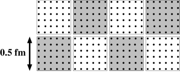
Figure 1: Two-dimensional cross-section of a $24\times 12^{3}$ lattice covered by non-overlapping $6^{4}$ blocks. Only such block divisions are considered that can be chessboard coloured and where the blocks have even sizes in all dimensions.

The development of the simulation algorithm that will be discussed here was guided by the general points listed above and by further considerations that are specific to QCD. As already mentioned, the blocks in the block lattice are taken to be fairly small, with sizes less than $1\,{\rm fm}$ or so. A strong infrared cutoff is then implied on the fluctuations of the block fields if Dirichlet boundary conditions are imposed (as we shall do). In particular, since QCD is asymptotically free, the theory becomes weakly coupled, and therefore easy to simulate, when restricted to the blocks. Treating the block fields separately is thus likely to be a good strategy.

Another property of the theory that may conceivably be exploited is related to the fact that the effective action

$$S_{\rm eff}=S_{\rm gauge}-2\ln\det D$$ (1)

is an approximately local functional of the SU(3) gauge potential $A_{\mu}^{a}$ (for simplicity a continuum notation is used in this section, where $S_{\rm gauge}$ denotes the Yang–Mills action and $D$ the massive Dirac operator, and it is assumed that there are two flavours of mass-degenerate quarks). To understand what approximate locality means and where it comes from, first note that, at non-zero distances $|x-y|$, the second variation of the effective action is given by

$${\delta^{2}S_{\rm eff}\over\delta A^{a}_{\mu}(x)\delta A^{b}_{\nu}(y)}=2\,{\rm tr}\{T^{a}\gamma_{\mu}S(x,y)T^{b}\gamma_{\nu}S(y,x)\},$$ (2)

where $S(x,y)$ stands for the quark propagator in the presence of the gauge field. The ellipticity of the Dirac operator implies that the quark propagator falls off roughly like $|x-y|^{-3}$ in the short-distance regime, and it usually decays even more rapidly at larger distances. Practitioners in lattice QCD have actually long been aware of the fact that quark propagators behave like this, for all representative gauge fields.

While this argumentation is not rigorous, it suggests that the gauge fields in distant blocks are only weakly coupled to each other. Starting with an algorithm that completely decouples the blocks, and treating the interactions between different blocks as a correction, may thus be an ansatz worth pursuing.

5 Block decomposition of the Dirac operator

In this and the following sections, only the standard Wilson theory will be considered, but all formulae generalize straightforwardly to the O($a$) improved theory. It is now also convenient to set the lattice spacing to unity. The lattice Dirac operator is then given by

$$D=\hbox{$1\over 2$}\left\{\gamma_{\mu}\left({\nabla\kern 0.5pt\smash{\raise 4.5pt\hbox{$\ast$}}\kern-5.5pt_{\mu}}+{\nabla_{\mu}}\right)-{\nabla\kern 0.5pt\smash{\raise 4.5pt\hbox{$\ast$}}\kern-5.5pt_{\mu}}{\nabla_{\mu}}\right\}+m_{0},$$ (3)

where, as usual, ${\nabla_{\mu}}$ and ${\nabla\kern 0.5pt\smash{\raise 4.5pt\hbox{$\ast$}}\kern-5.5pt_{\mu}}$ are the gauge-covariant forward and backward difference operators and $m_{0}$ is the bare quark mass.

On a block lattice such as the one shown in Fig. 1, the lattice is divided into two regions, the union $\Omega$ of all black blocks and the union $\Omega^{\ast}$ of all white blocks. The exterior boundaries of these domains, $\partial\Omega$ and $\partial\Omega^{\ast}$, are the sets of all points at distance $1$ from $\Omega$ and $\Omega^{\ast}$ respectively.

Now if the quark fields are written as a sum of two fields, $\psi=\psi_{\Omega}+\psi_{\Omega^{\ast}}$, with support in $\Omega$ and $\Omega^{\ast}$, the Dirac operator decomposes into four pieces according to

$$(D\psi)_{\Omega} = D_{\Omega}\psi_{\Omega}+D_{\partial\Omega}\psi_{\Omega^{\ast}},$$ (4)

$$(D\psi)_{\Omega^{\ast}} = D_{\partial\Omega^{\ast}_{\vphantom{1}}}\psi_{\Omega}+D_{\Omega^{\ast}_{\vphantom{1}}}\psi_{\Omega^{\ast}}.$$ (5)

The operator $D_{\Omega}$, for example, coincides with the Dirac operator on the domain $\Omega$, with Dirichlet boundary conditions at $\partial\Omega$, while $D_{\partial\Omega}$ is the sum of all hopping terms that go from $\partial\Omega$ to $\Omega$. A further decomposition into block operators $D_{\Lambda}$ is possible,

$$D_{\Omega}=\sum_{{\rm black\;blocks}\;\Lambda}D_{\Lambda},\qquad D_{\Omega^{\ast}_{\vphantom{1}}}=\sum_{{\rm white\;blocks}\;\Lambda}D_{\Lambda},$$ (6)

since $\Omega$ and $\Omega^{\ast}$ are unions of disjoint blocks $\Lambda$ that touch one another at the edges only.

Similarly to the familiar case of even–odd preconditioning, these equations go along with an exact factorization of the quark determinant,

$$\det D=\prod_{{\rm all\;blocks}\;\Lambda}\det D_{\Lambda}\times\det R,$$ (7)

where $R$ is an operator that acts on the subspace of quark fields supported on the boundary $\partial\Omega^{\ast}$. If the associated orthogonal projector is denoted by $P_{\partial\Omega^{\ast}}$, the operator is explicitly given by

$$R=1-P_{\partial\Omega^{\ast}}D_{\Omega}^{-1}D_{\partial\Omega}D_{\Omega^{\ast}_{\vphantom{1}}}^{-1}D_{\partial\Omega^{\ast}_{\vphantom{1}}}.$$ (8)

This expression looks a bit complicated, and one may have some doubts that the factorization (7) is useful. However, in view of the operator identity

$$R^{-1}=1-P_{\partial\Omega^{\ast}}D^{-1}D_{\partial\Omega^{\ast}_{\vphantom{1}}},$$ (9)

the solution of the equation $R\psi=\eta$, for example, is actually no more difficult to obtain than the solution of the Wilson–Dirac equation.

6 Preconditioned HMC algorithm

Starting from the factorization (7), the HMC algorithm [20] may now be set up as usual, with some modifications that will be explained below. Technically speaking, the block-diagonal operator $D_{\Omega}+D_{\Omega^{\ast}_{\vphantom{1}}}$ acts as a preconditioner for the HMC algorithm, with $R$ being the preconditioned Wilson–Dirac operator. This particular preconditioning is actually closely related to the classical Schwarz alternating procedure [18].

6.1 Block decoupling

For two mass-degenerate flavours of quarks, the pseudo-fermion action associated to the determinants in eq. (7) is given by

$$S_{\rm pf}=\sum_{{\rm all\;blocks}\;\Lambda}\left\|\hat{D}_{\Lambda}^{-1}\phi_{\Lambda}\right\|^{2}+\left\|R^{-1}\chi\right\|^{2}.$$ (10)

In this expression the block operators $D_{\Lambda}$ have been replaced by their even–odd preconditioned form $\hat{D}_{\Lambda}$ (which is permissible since the determinants are the same). The fields $\phi_{\Lambda}$ thus reside on the even sites in the blocks $\Lambda$ and $\chi$ is supported on $\partial\Omega^{\ast}$.

As explained before, one of the algorithmic strategies is to decouple the gauge-field variables in different blocks as much as possible. A partial decoupling is easily achieved by updating only a subset of all gauge-field variables in each update cycle. With respect to the field variables residing on the links shown in Fig. 2, for example, the gauge action decomposes into a sum of block actions, and the same is trivially true for the block terms in eq. (10). The field variables in different blocks are then still coupled to each other through the last term in the pseudo-fermion action (the one involving the operator $R$), but as will become clear shortly, this interaction is relatively weak.

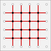
Figure 2: Along the molecular-dynamics trajectories, only the field variables on the active links (thick lines) in the blocks are evolved, while all other link variables are kept fixed. In this way a partial decoupling of the gauge-field variables in different blocks is achieved.

Evidently, an algorithm that updates always the same subset of field variables is not ergodic, but this problem can be overcome by alternating between different block divisions or simply by applying a random space–time translation to the gauge field after every update cycle. In the course of the simulation all link variables are then treated equally.

6.2 Molecular-dynamics forces

Following the standard rules, the trajectories in field space are obtained by solving the molecular-dynamics equations

$${{\rm d}\over{\rm d}t}\,U(x,\mu) = \Pi(x,\mu)U(x,\mu),$$ (11)

$${{\rm d}\over{\rm d}t}\,\Pi(x,\mu) = -F_{\rm G}(x,\mu)-F_{\Lambda}(x,\mu)-F_{R}(x,\mu),$$ (12)

for the gauge-field variables $U(x,\mu)$ on the active links and their canonical momenta $\Pi(x,\mu)$. The forces $F_{\rm G}$, $F_{\Lambda}$ and $F_{R}$ in these equations derive from the gauge action, the block terms and the last term in the pseudo-fermion action (10), respectively.

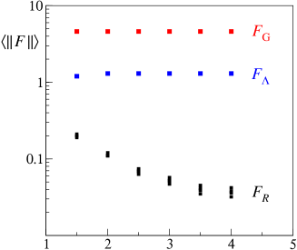
Figure 3: Average magnitude of the forces $F_{G}$, $F_{\Lambda}$ and $F_{R}$ at the end of the molecular-dynamics trajectories as a function of the distance from the block boundary (simulation of the O($a$) improved theory on a $32\times 16^{3}$ lattice divided into $8^{4}$ blocks). Only $F_{R}$ shows a non-negligible dependence on the quark mass (lowest four points at each distance).

An important observation is now that these forces have widely different magnitudes. This is so on all lattices considered so far, independently of the quark masses and of whether O($a$) corrections are included or not. Typically the situation is as shown in Fig. 3, where $F_{\rm G}$ is about $4$ times larger than $F_{\Lambda}$, which is more than $6$ times larger than $F_{R}$. Moreover, even though the bare current-quark mass ranged from $14$ to $70$ MeV in this study, there is hardly any mass dependence seen on the scale of the plot.

To some extent, at least, these empirical findings can be understood theoretically (cf. Sect. 4). The block forces $F_{\Lambda}$, for example, are protected from large fluctuations and a significant quark-mass dependence, because there is a strong infrared cutoff on the spectrum of the block Dirac operators. Somewhat less obvious is perhaps the suppression of the third force

$$F_{R}(x,\mu)=2\,{\rm Re}\,\!\left(R^{-1}\chi,D^{-1}\delta^{U}_{x,\mu}DD^{-1}D_{\partial\Omega^{\ast}}\chi\right).$$ (13)

This formula shows, however, that the force involves two quark propagators that go from the boundaries of the blocks to the point $x$ where the force is to be evaluated. The decay properties of the quark propagator then suggest that the force should be small, particularly so at the points $x$ that are well inside the blocks.

6.3 Integration scheme

The widely used numerical integration schemes for the molecular-dynamics equations divide the integration range $0\leq t\leq\tau$ into $N$ steps of size $\epsilon=\tau/N$, and update the momenta and the link variables step by step. Evidently the computational cost of the integration (and thus of the simulation) is inversely proportional to the step size.

When the evolution is driven by several forces of different magnitudes, as in the present case, it is possible to use larger step sizes for the smaller forces. This was first pointed out by Sexton and Weingarten [27] many years ago, and the idea was more recently revived by Peardon and Sexton [16], who suggested to split the forces into high- and low-frequency parts, where the latter are integrated at a lower speed.

Here the multiple step-size integration method can be applied straightforwardly since the total force is already split in parts. It seems reasonable to choose the associated step sizes $\epsilon_{0},\epsilon_{1},\epsilon_{2}$ such that

$$\epsilon_{0}\|F_{\rm G}\|\simeq\epsilon_{1}\|F_{\Lambda}\|\simeq\epsilon_{2}\|F_{R}\|.$$ (14)

This rule works well in practice, and in all simulations reported later the step sizes were as in Fig. 4. In this way the computational cost per trajectory is potentially reduced by a large factor, because the block-interaction force $F_{R}$, which is by far the most difficult to calculate at small quark masses, is now also the least often computed force.

Figure 4: Division of the integration interval into steps of size $\epsilon_{0}$ (small tick marks). The multiple step-size integration requires the gauge force $F_{\rm G}$ to be computed at all ticks, the block forces $F_{\Lambda}$ at the middle-size ticks and the block-interaction force $F_{R}$ at the large ticks only.

7 Simulations of two-flavour QCD

Numerical studies of the Schwarz-preconditioned HMC algorithm started about one and a half years ago, using $8$ nodes of a PC cluster at the Institute for Theoretical Physics at Berne [19]. The algorithm is now well understood and more extensive simulations, on a cluster with $64$ nodes at the Fermi Institute in Rome, are being performed by a collaboration based at CERN and the University of Rome “Tor Vergata” [25].

The parameters of the simulations carried out so far are listed in Table 1. In all cases the standard Wilson theory was considered and the trajectory length $\tau$ was set to $0.5$. Along the trajectories the lattice Dirac equation on the blocks and the full lattice was solved accurately enough to guarantee the reversibility of the molecular-dynamics evolution at a level better than $10^{-9}$. For the solution of the Dirac equation on the full lattice, a highly parallel Schwarz-preconditioned solver was used [17].

Lattice	$\beta$	$\kappa$	$\sim m/m_{\rm s}$	Block size	$\tau/\epsilon_{2}$	$N_{\rm traj}$	$P_{\rm acc}$
$32\times 24^{3}$	$5.6$	$0.15750$	$0.93$	$8\times 6^{2}\times 12$	$5$	$6400$	$0.80$
		$0.15800$	$0.48$		$6$	$9500$	$0.80$
		$0.15825$	$0.30$		$10$	$9400$	$0.86$
		$0.15835$	$0.17$		$16$	$5000$	$0.91$
$64\times 32^{3}$	$5.8$	$0.15410$	$0.75$	$16\times 8^{3}$	$8$	$5000$	$0.86$
		$0.15440$	$0.38$		$10$	$5050$	$0.89$

Table 1: Simulations were performed at several values of the inverse gauge coupling $\beta=6/g_{0}^{2}$ and the hopping parameter $\kappa=(8+2m_{0})^{-1}$. The lowest current quark mass $m$ reached in these runs was about a sixth of the physical strange-quark mass $m_{\rm s}$. In the last two columns, the number of trajectories generated after thermalization and the average acceptance rate are reported.

In physical units the lattice spacing is estimated to be about $0.080$ fm at $\beta=5.6$ and $0.064$ fm at $\beta=5.8$ . All simulated lattices thus have a spatial size close to $2$ fm, and a comparison of the simulation results obtained on the $32\times 24^{3}$ and the $64\times 32^{3}$ lattice should therefore provide some clues as to how large the lattice effects are at these lattice spacings. Further simulations on the big lattice are still required, however, to match the range of quark masses covered on the small one.

An important experience made in these simulations is that the number $\tau/\epsilon_{2}$ of the integration steps at which the block-interaction force $F_{R}$ must be computed can be taken to be fairly small. Moreover, to keep the acceptance rates high when the quark mass is lowered, a moderate increase in the step numbers turns out to be sufficient. The performance of the algorithm will be discussed later, but these low numbers and the fact that the simulations could be performed on relatively small computers already show that the algorithm works very well.

8 Pion mass and decay constant

Some of the simulations reported here were performed at fairly low quark masses, and the question may now be asked whether contact with chiral perturbation theory can be made at these points. In the case of the pion mass $m_{\pi}$, for example, two-flavour chiral perturbation theory predicts

$$m_{\pi}^{2} = M^{2}R_{\pi},\qquad M^{2}\equiv 2Bm,$$ (15)

$$R_{\pi} = 1+{M^{2}\over 32\pi^{2}F^{2}}\ln(M^{2}/\Lambda_{\pi}^{2})+\ldots,$$ (16)

where $m$ denotes the current quark mass, $F$ the pion decay constant in the chiral limit, $B$ another constant related to the chiral condensate, and $\Lambda_{\pi}$ a scale that characterizes the strength of the one-loop chiral corrections in this formula [29].

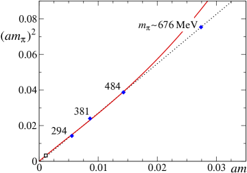
Figure 5: Simulation results for the pion mass $m_{\pi}$ on the $32\times 24^{3}$ lattice, plotted versus the current quark mass $m$ in lattice units. The dotted line is a linear fit of all four data points. Below $m_{\pi}\simeq 500\,{\rm MeV}$, one-loop chiral perturbation theory fits the data equally well (full line). The point represented by an open square is obtained by extrapolation to the physical pion mass.

In lattice QCD the pion mass and the current quark mass are usually extracted from the correlation functions of the isovector axial current and density. The data points obtained in this way on the $32\times 24^{3}$ lattices are plotted in Fig. 5. They all lie on a straight line, which passes through the origin within errors, and so it seems that the data leave no room for chiral loop corrections.

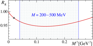
Figure 6: Plot of the one-loop chiral correction factor (8.2) as a function of $M^{2}=2Bm$, using the values of $F$ and $\Lambda_{\pi}$ quoted by Gasser and Leutwyler [29]. In the shaded range, $R_{\pi}$ changes by less than $1\%$ and $m_{\pi}^{2}$ is practically a linear function of the quark mass.

This is not obviously so, however, because the loop corrections could be very small. In real-world QCD, for example, the scale $\Lambda_{\pi}$ is expected to be such that [29]

$$\left.\ln(\Lambda_{\pi}^{2}/M^{2})\right|_{M=140\,{\rm MeV}}\simeq 2.9\pm 2.4.$$ (17)

Using this estimate and setting $F=88$ MeV, the one-loop expression (16) for the correction factor $R_{\pi}$ turns out to be practically constant in the relevant range of pion masses (see Fig. 6). The pion mass squared is thus predicted to be a nearly linear function of the quark mass in this range, although with a slope about $4\%$ lower than $2B$. It is then not too surprising that one-loop chiral perturbation theory fits the data plotted in Fig. 5 if the point at the largest mass is omitted. Moreover, the values of the fit parameters $B$ and $\Lambda_{\pi}$ come out to be close to the phenomenologically expected ones.

The situation in the case of the pion decay constant $F_{\pi}$ is qualitatively similar, but the one-loop correction in the chiral expansion

$$F_{\pi}=F\left\{1-{M^{2}\over 16\pi^{2}F^{2}}\ln(M^{2}/\Lambda_{F}^{2})+\ldots\right\}$$ (18)

tends to be larger than in eq. (16) by a factor $4$ or so. On the lattice the data for the decay constant must be renormalized before they can be compared with this formula. Since the renormalization factor $Z_{A}$ is currently not known, it was estimated using “tadpole-improved” perturbation theory. Moreover, a small finite-volume correction, computed to one-loop order of chiral perturbation theory [30], was applied to the data.

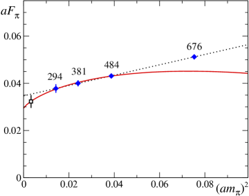
Figure 7: Simulation results for the pion decay constant $F_{\pi}$ on the $32\times 24^{3}$ lattice, plotted versus the pion mass squared in lattice units. The curves are linear and chiral fits of the data as in Fig. 5.

Within statistical errors, the corrected data shown in Fig. 7 lie on a straight line. The data are also compatible with the chiral formula (18) if the point at the largest mass is discarded and if $F$ and $\Lambda_{F}$ are treated as free fit parameters. As it turns out, the fit result for the latter comes out to be well within the range

$$\left.\ln(\Lambda_{F}^{2}/M^{2})\right|_{M=140\,{\rm MeV}}\simeq 4.6\pm 0.9$$ (19)

quoted by Gasser and Leutwyler [29], while the value obtained for the decay constant after extrapolation to the physical point, $\left.F_{\pi}\right|_{M=140\,{\rm MeV}}=80(7)$ MeV, is a bit lower than expected in real-world QCD. This result should not be taken too seriously, however, since there are still many uncontrolled systematic errors in this calculation. In particular, there can be large lattice-spacing effects.

The conclusion is then that the simulation results for $m_{\pi}$ and $F_{\pi}$ obtained on the $32\times 24^{3}$ lattice are compatible with one-loop chiral perturbation theory, within errors and up to pion masses of about $500$ MeV. On the other hand, since the data can also be fitted by straight lines, the presence of the chiral logarithms has not been unambiguously demonstrated. The discussion also showed, however, that their effects are very small, partly because of accidental numerical cancellations. More extensive simulations will therefore be required if chiral perturbation theory is to be matched at this level of precision.

9 Large-lattice experiences

As already mentioned, the simulations of the $64\times 32^{3}$ lattice performed so far will have to be extended to smaller quark masses to match the range of masses covered on the smaller lattice. There are, however, a number of interesting remarks that can be made at this point.

To a first approximation, the simulation algorithm performs equally well on the two lattices. In particular, good acceptance rates were achieved with similarly low step numbers $\tau/\epsilon_{2}$. The larger volume of the big lattice actually appears to have a stabilizing effect on the simulations (see fig. 8). The deficit $\Delta H$ of the molecular-dynamics Hamiltonian at the end of the trajectories, for example, remained bounded essentially between $-1$ and $+1$ in all cases, and the iteration numbers $N_{\rm GCR}$ of the solver used for the full-lattice Dirac equation fluctuated with standard deviations of $3$ to $5\%$ only.

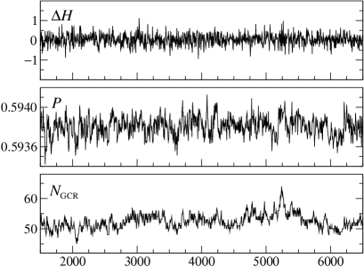
Figure 8: Histories of the energy deficit $\Delta H$, the average plaquette $P$ and the average solver iteration number $N_{\rm GCR}$ as functions of the trajectory number ($64\times 32^{3}$ lattice, simulation parameters as given on the last line of Table 1). Only the values at every 5th trajectory are plotted.

In general, simulating large lattices pays off in many ways. A common experience is that the a priori statistical errors tend to be smaller on these lattices and that a significant further reduction in the errors is seen when the correlation functions of interest are averaged over several distant source points. Moreover the time dependence of the correlation functions can be followed up to larger time separations, which is particularly helpful when the masses of the vector mesons, the baryons and other heavy particles are to be calculated (see Fig. 9).

Note, incidentally, that the mass gap $W_{\rho}$ in the $\rho$-channel does not necessarily coincide with the mass of the $\rho$-resonance. The virtual mixing with the isovector two-pion states actually sets in as soon as the gap is greater than $2m_{\pi}$, and this leads to volume-dependent energy shifts that can be fairly large [31].

10 Performance figures and timings

Contrary to what may be assumed, the performance of a simulation algorithm is not readily established and comparisons of different algorithms may easily be misleading. There are a number of points that should be taken into account:

• In practice the efficiency of an algorithm depends on the lattice parameters, the program and the computer. A particular algorithm may be a good choice for simulations of coarse lattices, for example, but less competitive at smaller lattice spacings.

• Modern algorithms tend to have many tunable parameters that must be properly adjusted, on each lattice, to achieve a good efficiency. Performing many simulations for tuning purposes alone may not be possible, however, and good algorithms should thus have a transparent and soft parameter dependence.

• The relevant autocorrelation times are often difficult to determine reliably. Moreover, when the available data series are not exceedingly long, the calculation of autocorrelation times invariably involves a certain amount of subjective judgement.

In particular, saying that algorithm $A$ is five times faster than algorithm $B$, without further qualifications, is almost certainly a meaningless statement.

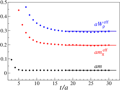
Figure 9: Plot of the current-quark mass $m$, the pion mass $m_{\pi}$ and the mass gap $W_{\rho}$ in the $\rho$-meson channel ($64\times 32^{3}$ lattice, simulation parameters as given on the next-to-last line of table 1). The values shown are effective masses in lattice units, obtained from the appropriate correlation functions at times $t$ and $t-a$.

When a simulation algorithm spends most of the time on the solution of the Dirac equation on the full lattice, as is the case here, a useful measure of the computational cost is the number of times the solver has to be called before the next statistically independent field configuration is obtained. A cost figure of this kind is

$$\quad\nu=10^{-3}\left(2N_{2}+3\right)\tau_{\rm int}[P],\qquad N_{2}=\tau/\epsilon_{2},$$ (20)

where $\tau_{\rm int}[P]$ denotes the integrated autocorrelation time of the plaquette. Evidently $\nu$ is independent of the solver, the program and the computer that are used for the simulation.

Lattice	$\beta$	$c_{\rm sw}$	$am$	$\tau_{\rm int}[P]$	$\nu$
$32\times 16^{3}$	$5.3$	$1.9095$	$0.035$	$56(26)$	$0.84(39)$
			$0.021$	$14(4)\kern 4.50002pt$	$0.27(8)\kern 4.50002pt$
			$0.011$	$21(6)\kern 4.50002pt$	$0.40(11)$
			$0.007$	$17(5)\kern 4.50002pt$	$0.39(12)$
$32\times 24^{3}$	$5.6$	$0.0$	$0.027$	$53(22)$	$0.69(29)$
			$0.014$	$33(11)$	$0.50(17)$
			$0.009$	$27(10)$	$0.62(23)$
			$0.006$	$21(5)\kern 4.50002pt$	$0.74(18)$
$64\times 32^{3}$	$5.8$	$0.0$	$0.019$	$16(3)\kern 4.50002pt$	$0.30(6)\kern 4.50002pt$
			$0.011$	$13(2)\kern 4.50002pt$	$0.30(5)\kern 4.50002pt$

Table 2: Estimates of the integrated autocorrelation time of the plaquette (in numbers of trajectories of length $\tau=0.5$) and of the cost figure $\nu$ [eq. (10.1)]. The results listed on the first few lines refer to the O($a$) improved theory, with non-perturbatively tuned coeffcient $c_{\rm sw}$ of the Sheikholeslami–Wohlert term [32].

Within errors, the cost figures listed in Table 2 do not show any obvious dependence on the quark mass or the lattice size. Moreover, whether O($a$) improvement is switched on or not does not appear to make a big difference. An exceptional case are the two runs on the $64\times 32^{3}$ lattice, where the cost figures reflect the high degree of stability of the simulations mentioned before.

Much larger values of $\nu$ are common to all previous simulations of two-flavour QCD. In a study of the O($a$) improved theory conducted by the UKQCD collaboration [11], for example, using the even–odd preconditioned HMC algorithm, the cost figure on a $32\times 16^{3}$ lattice at $m_{\pi}\simeq 420$ MeV was $5.5(11)$. Significantly smaller masses were reached by the CP–PACS collaboration on a coarse $24\times 12^{3}$ lattice [15], and in these simulations, $\nu$ ranged from $9.4(18)$ at $m_{\pi}\simeq 398$ MeV to $29(10)$ at $m_{\pi}\simeq 255$ MeV. From this purely algorithmic point of view, the new algorithm is thus much more efficient than the algorithms previously used, particularly so at small quark masses.

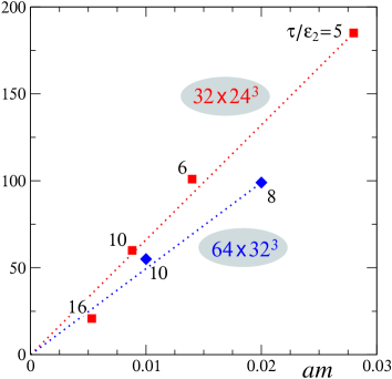
Figure 10: Number of accepted gauge-field configurations generated per day at the simulation points listed in table 1. All simulations were performed on commodity PC clusters, using $8$ and $32$ nodes, respectively, for the $32\times 24^{3}$ and $64\times 32^{3}$ lattices.

In practice the computer time required for a particular simulation also depends on the specific capabilities of the available computers and the efficiency of the program. So far the algorithm has been implemented on PC clusters, and it performs very well on these machines (see Fig. 10). Moreover, the timings show that the algorithm scales favourably with the quark mass and the lattice size, a property that should be largely independent of the computer and the program.

11 Conclusions

The important qualitative message of this talk is that numerical simulations of lattice QCD with light Wilson quarks are much less “expensive” than previously estimated. Lattices as large as $96\times 48^{3}$, for example, with lattice spacings $a=0.06$–$0.08$ fm and at pion masses from, say, $200$ to $500$ MeV, should now be accessible using a (current) PC cluster with a few hundred nodes. As a result contact with chiral perturbation theory can be made at lattice spacings where the residual lattice effects are expected to be small.

After having passed many tests successfully, the use of the Schwarz-preconditioned HMC algorithm can be recommended without reservation if large lattices, with lattice spacings $a\leq 0.1\,{\rm fm}$, are to be simulated. First studies now also confirm that the efficiency of the algorithm is preserved when O($a$) improvement is switched on. There appears to be very little difference here, and it also seems unlikely that the addition of six-link terms to the gauge action [33]–[36] will slow down the simulations significantly. Some thought may have to be given, however, to which is the best way to include the strange sea quark, although this quark is so heavy that one may be able to do with a preconditioned PHMC algorithm [37, 38].

Not many physics issues were touched in this talk, but there is a wide range of topics that may now be addressed in a conceptually solid framework, including pion scattering, the $\rho$-resonance, the properties of the nucleons and the charmed mesons, to mention just the obvious ones. Sometimes it seems that the most difficult question in these days is: What should we compute first?

Many results presented here were obtained together with Luigi Del Debbio, Leonardo Giusti, Roberto Petronzio and Nazario Tantalo, whom I would like to thank for helpful discussions and a pleasant collaboration. The numerical simulations were performed on a PC cluster at the Institut für Theoretische Physik der Universität Bern, which was funded in part by the Schweizerischer Nationalfonds, and on another PC cluster at the Fermi Institute in Rome. I wish to thank all these institutions for their support.

References

- [1] K. G. Wilson, Confinement of quarks, Phys. Rev. D10 (1974) 2445
- [2] B. Sheikholeslami and R. Wohlert, Improved continuum limit lattice action for QCD with Wilson fermions, Nucl. Phys. B259 (1985) 572
- [3] M. Lüscher, S. Sint, R. Sommer and P. Weisz, Chiral symmetry and improvement in lattice QCD, Nucl. Phys. B478 (1996) 365 [hep-lat/9605038]
- [4] SESAM and TL Collaborations, Th. Lippert et al., SESAM and TL results for Wilson action: A status report, Nucl. Phys. B (Proc. Suppl.) 60A(1998) 311 [hep-lat/9707004]
- [5] TL Collaboration, N. Eicker et al., Light and strange hadron spectroscopy with dynamical Wilson fermions, Phys. Rev. D59 (1999) 014509 [hep-lat/9806027]
- [6] TL Collaboration, G. S. Bali et al., Static potentials and glueball masses from QCD simulations with Wilson sea quarks, Phys. Rev. D62 (2000) 054503 [hep-lat/0003012]
- [7] N. Eicker, Th. Lippert, B. Orth and K. Schilling, Light quark masses with Wilson fermions, Nucl. Phys. B (Proc. Suppl.) 106 (2002) 209 [hep-lat/0110134]
- [8] B. Orth, Th. Lippert and K. Schilling, Finite-size effects in lattice QCD with dynamical Wilson fermions, Phys. Rev. D72 (2005) 014503 [hep-lat/0503016]
- [9] UKQCD Collaboration, C. R. Allton et al., Light hadron spectroscopy with O(a) improved dynamical fermions, Phys. Rev. D60 (1999) 034507 [hep-lat/9808016]
- [10] UKQCD Collaboration, C. R. Allton et al., Effects of non-perturbatively improved dynamical fermions in QCD at fixed lattice spacing, Phys. Rev. D65 (2002) 054502 [hep-lat/0107021]
- [11] UKQCD Collaboration, C. R. Allton et al., Improved Wilson QCD simulations with light quark masses, Phys. Rev. D70 (2004) 014501 [hep-lat/0403007]
- [12] CP–PACS Collaboration, A. Ali Khan et al., Dynamical quark effects on light quark masses, Phys. Rev. Lett. 85 (2000) 4674 [E: ibid. 90 (2003) 029902] [hep-lat/0004010]
- [13] CP–PACS Collaboration, A. Ali Khan et al., Light hadron spectroscopy with two flavors of dynamical quarks on the lattice, Phys. Rev. D65 (2002) 054505 [E: ibid. D67 (2003) 059901] [hep-lat/0105015]
- [14] JLQCD Collaboration, S. Aoki et al., Light hadron spectroscopy with two flavors of O(a)-improved dynamical quarks, Phys. Rev. D68 (2003) 054502 [hep-lat/0212039]
- [15] CP–PACS Collaboration, Y. Namekawa et al., Light hadron spectroscopy in two-flavor QCD with small sea quark masses, Phys. Rev. D70 (2004) 074503 [hep-lat/0404014]
- [16] TrinLat Collaboration, M. J. Peardon and J. C. Sexton, Multiple molecular dynamics time-scales in Hybrid-Monte-Carlo fermion simulations, Nucl. Phys. B (Proc. Suppl.) 119 (2003) 985 [hep-lat/0209037]
- [17] M. Lüscher, Lattice QCD and the Schwarz alternating procedure, JHEP 0305 (2003) 052 [hep-lat/0304007]
- [18] M. Lüscher, Solution of the Dirac equation in lattice QCD using a domain-decomposition method, Comput. Phys. Commun. 156 (2004) 209 [hep-lat/0310048]
- [19] M. Lüscher, Schwarz-preconditioned HMC algorithm for two-flavour lattice QCD, Comput. Phys. Commun. 165 (2005) 199 [hep-lat/0409106]
- [20] S. Duane, A. D. Kennedy, B. J. Pendleton and D. Roweth, Hybrid Monte Carlo, Phys. Lett. B195 (1987) 216
- [21] M. Hasenbusch, Speeding up the Hybrid-Monte-Carlo algorithm for dynamical fermions, Phys. Lett. B519 (2001) 177 [hep-lat/0107019]
- [22] M. Hasenbusch and K. Jansen, Speeding up lattice QCD simulations with clover-improved Wilson fermions, Nucl. Phys. B659 (2003) 299 [hep-lat/0211042]
- [23] ALPHA Collaboration, M. Della Morte et al., Simulating the Schrödinger functional with two pseudo-fermions, Comput. Phys. Commun. 156 (2003) 62 [hep-lat/0307008]
- [24] C. Urbach, K. Jansen, A. Shindler and U. Wenger, HMC algorithm with multiple time scale integration and mass preconditioning, hep-lat/0506011
- [25] L. Del Debbio, L. Giusti, M. Lüscher, R. Petronzio and N. Tantalo, in preparation
- [26] Y. Saad, Iterative methods for sparse linear systems, 2nd ed. (SIAM, Philadelphia, 2003); see also http://www-users.cs.umn.edu/~saad/
- [27] J. C. Sexton and D. H. Weingarten, Hamiltonian evolution for the Hybrid-Monte-Carlo algorithm, Nucl. Phys. B380 (1992) 665
- [28] R. Sommer, A new way to set the energy scale in lattice gauge theories and its applications to the static force and in SU(2) Yang-Mills theory, Nucl. Phys. B411 (1994) 839 [hep-lat/9310022]
- [29] J. Gasser and H. Leutwyler, Chiral perturbation theory to one loop, Ann. Phys. 158 (1984) 142
- [30] J. Gasser and H. Leutwyler, Light quarks at low temperatures, Phys. Lett. B184 (1987) 83
- [31] M. Lüscher, Signatures of unstable particles in finite volume, Nucl. Phys. B364 (1991) 237
- [32] ALPHA Collaboration, K. Jansen and R. Sommer, O() improvement of lattice QCD with two flavors of Wilson quarks, Nucl.Phys. B530 (1998) 185 [E: ibid. B643 (2002) 517] [hep-lat/9803017]
-
[33]
Y. Iwasaki,
Renormalization group analysis of lattice theories
and improved lattice action.
2. Four-dimensional non-abelian SU() gauge model, Tsukuba preprint UTHEP-118 (1983) - [34] Y. Iwasaki, Renormalization group analysis of lattice theories and improved lattice action: Two-dimensional nonlinear O() sigma model, Nucl. Phys. B258 (1985) 141
- [35] M. Lüscher and P. Weisz, On-shell improved lattice gauge theories, Commun. Math. Phys. 97 (1985) 59 [E: ibid. 98 (1985) 433]
- [36] M. Lüscher and P. Weisz, Computation of the action for on-shell improved lattice gauge theories at weak coupling, Phys. Lett. B158 (1985) 250
- [37] P. de Forcrand and T. Takaishi, Fast fermion Monte Carlo, Nucl. Phys. B (Proc. Suppl.) 53 (1997) 968 [hep-lat/9608093]
- [38] R. Frezzotti and K. Jansen, A polynomial Hybrid-Monte-Carlo algorithm, Phys. Lett. B402 (1997) 328 [hep-lat/9702016]