The critical end point of quantum chromodynamics

Abstract:

We investigate the critical end point (CEP) of QCD with two flavours of light dynamical quarks at finite lattice cutoff $a=1/4T$ using a Taylor expansion of the baryon number susceptibility. We find a strong volume dependence of the position of the critical end point. In the large volume limit we obtain $T^{E}/T_{c}\approx 0.95$ and $\mu_{B}^{E}/T^{E}\approx 1.1$, where $T_{c}$ is the cross over temperature at zero chemical potential, and $T^{E}$ and $\mu_{B}^{E}$ are the temperature and the baryon chemical potential at the critical end point. The small value of $\mu_{B}^{E}$ places it in the range of observability in energy scans at the RHIC.

PoS(LAT2005)160

1 Finding the CEP by Taylor Expansion

In QCD with two flavours of quarks, the pressure and its Taylor expansion are

$$P(T,\mu_{u},\mu_{d})\equiv\left(\frac{T}{V}\right)\log Z(T,\mu_{u},\mu_{d})=P(T,0,0)+\sum_{n_{u},n_{d}}\chi_{n_{u},n_{d}}\frac{\mu_{u}^{n_{u}}}{n_{u}!}\frac{\mu_{d}^{n_{d}}}{n_{d}!}$$ (1)

where $T$ is the temperature, $\mu_{u,d}$, the chemical potentials for each flavour (since weak interactions are neglected, flavours are exactly conserved), $V$, the volume, $Z$, the partition function, and the Taylor expansion is around $\mu_{u}=\mu_{d}=0$. The Taylor coefficients are called quark number susceptibilities (QNS). The coefficients of order higher than 2 were called non-linear susceptibilities (NLS) in [1]. Most lattice computations are performed in the flavour symmetric limit, $m_{u}=m_{d}$, which forces the coefficients to have the symmetry $\chi_{nm}=\chi_{mn}$. Also, CP symmetry forces $\chi_{n,N-n}=0$ whenever $N$ is odd.

We are interested in the critical end point in the plane of $T$ and the baryon chemical potential $\mu_{B}=3\mu_{u}=3\mu_{d}$. The second derivative

$$\chi_{20}(T,\mu_{B})=\left.\frac{\partial^{2}P}{\partial\mu_{u}^{2}}\right|_{\mu_{u}=\mu_{d}=\mu_{B}/3}$$ (2)

diverges at the critical point in the thermodynamic limit. We construct the Taylor series for this QNS from (1). In [2] we extract the Taylor coefficients of $\chi_{20}(T,\mu_{B})$ from lattice simulations in order to estimate the CEP. Note that we scan along lines of constant $T$. At the CEP the Taylor expansion in (2) would break down. Hence, the radius of convergence of the series, in the thermodynamic limit, would give the position of the CEP provided that there is no other critical point nearer to $\mu_{u}=\mu_{d}=0$.

Our analysis involves examination of finite volume effects in $\chi_{20}(T,\mu_{B})$. On any finite volume, as one scans along a line of constant $T$, one sees a peak in the QNS. With increasing volume one sees larger and sharper peaks, which go smoothly into the non-analytic divergence in the thermodynamic limit. This implies an interesting behaviour for the Taylor coefficients on finite volumes. Estimates of the radius of convergence from terms up to some order $N_{;}(V)$ should indicate a finite value; but terms of order greater than $N_{;}(V)$ would show a growth in the radius of convergence. With increasing $V$ one should observe $N_{;}(V)$ to be increasing. Estimates of the radius of convergence have to be performed, perforce, at finite $V$, and therefore only the estimates for orders less than $N_{;}(V)$ should be used, and continued to the thermodynamic limit using standard finite size scaling methods.

The main systematic errors in the location of CEP by lattice methods are due to three sources— lattice spacing effects, finite volume effects, quark mass effects. In this work we show that finite volume effects can be controlled when ${\cal V}=m_{\pi}V^{1/3}>5$. By working in the large volume region and taking small quark masses such that $m_{\pi}/m_{\rho}=0.3$ (close to the physical value) we are able to control the last two sources of errors simultaneously for the first time. Lattice spacing errors will be considered later. Our simulation parameters are listed in [2]. We expand $P$ to 8th order in $\mu_{B}$.

2 Optimizing the computations

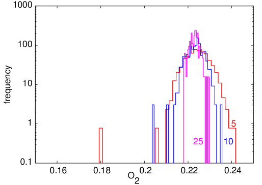
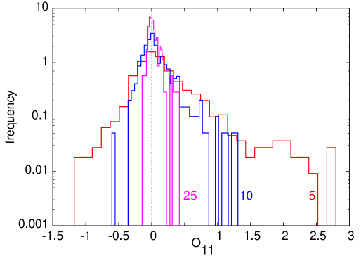
Figure 1: The distribution of estimators of the traces involved in (a) $\chi_{20}$ and (b) $\chi_{11}$ on one configuration at $0.8T_{c}$ by Gaussian distributed noise vectors. The different histograms in each case are labeled by the number of vectors used to make one measurement. Noise in the measurement of $\chi_{11}$ arises from the significantly larger spread of the second (highly non-Gaussian) histogram with a much smaller mean, and therefore requires many more vectors to control.

Every derivative of $\log Z$ with respect to $\mu$ lands on the Dirac determinant, since this is the part of the measure which contains $\mu$. Every derivative of the determinant of a matrix creates an inverse power of the matrix, i.e., a quark propagator in this example. Thus, when Taylor series are examined at order $N$, they may contain terms containing up to $N$ propagators. On every gauge configuration one is therefore required to construct fermion traces with many propagators, implying a need for multiple Dirac matrix inversions. The way to optimize the number of inversions is to map this problem on to a computer science problem called the “Steiner problem” [3]. Details are given in [2].

Fermion traces are obtained using the usual stochastic method— random vectors are drawn from some ensemble (usually Gaussian or $Z_{2}$), the expectation of the operator is found on each vector and the average is found over the noise ensemble. Optimization involves choosing the ensemble and the number of vectors. We found that for this specific purpose the Gaussian ensemble is superior to the $Z_{2}$ noise ensemble. The number of vectors needed increases with the order, and at each order Fermion-line-disconnected operators require more vectors than connected operators.

Since multiple matrix inversions are required to on each gauge configurations, one may expect a priori that some preconditioning or reuse of vectors may improve the performance of the inverter. However, it turns out that the extra arithmetic effort involved in this is comparatively large, and leads to gains of around 10% (with a less sparse Dirac operator, i.e., with improved actions, there may be more gain). We therefore did not optimize the inversion in this manner. The main optimization of the CG inverter was to tune the stopping criterion.

We measured the autocorrelations of the Wilson line and the quark condensate during the R-algorithm run, and chose to analyze only one configuration per autocorrelation time, gathering statistics of 50–100 configuration at each coupling on every lattice size. Since autocorrelations are large in the vicinity of the QCD crossover temperature, $T_{c}$, it took massive computational effort to generate sufficient statistics in this interesting region. The effort required in the measurements was significantly smaller.

3 Non-linear susceptibilities

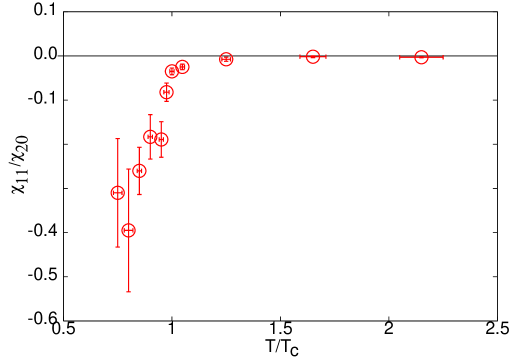
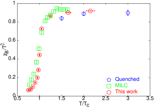
Figure 2: The first panel shows the ratio $\chi_{11}/\chi_{20}$ as a function of $T/T_{c}$. The second shows the scaled value of $\chi_{20}$ from our computation (see text for details) compared to data from [5] and quenched QCD [6].

Different systematics are seen for non-linear susceptibilities (NLS) in the three regions, well below $T_{c}$, near $T_{c}$ and well above $T_{c}$ [4]. An example is provided by the ratio $\chi_{11}/\chi_{20}$ which measures the importance of sign fluctuations in the partition function at small chemical potential. This is of order unity at $0.75T_{c}$, and decreases rapidly in the region near $T_{c}$, becoming of the order of $10^{-3}$ at large $T$ (see Figure 2). $\chi_{20}$ itself crosses over from a small value below $T_{c}$ to a much larger values above $T_{c}$. In Figure 2 the value shown is the observed value scaled by a factor which would transform measurements of $\chi_{20}$ in the quenched theory at the same lattice spacing into the continuum. We have argued before that this procedure is within 5—10% of the true continuum limit. Taking into consideration this uncertainty, and differences in quark masses and lattice volumes, the values are in agreement with the $N_{t}=8$ computations with improved staggered quarks of [5].

Well above $T_{c}$ there is a hierarchy of values of the NLS which is consistent with weak-coupling power counting rules. In the vicinity of $T_{c}$ these rules break down, and some of the NLS peak. These peaks are found to be due to one particular class of operators, which measure fluctuations of the fermion-line-connected operator, ${\cal O}_{2}$, contributing to $\chi_{20}$ [4].

4 The CEP

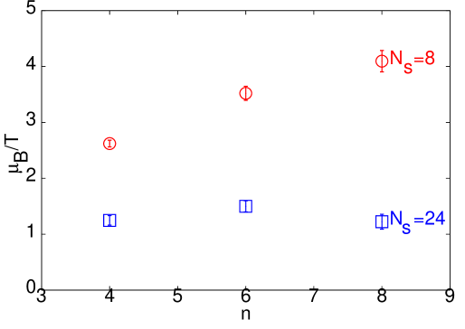
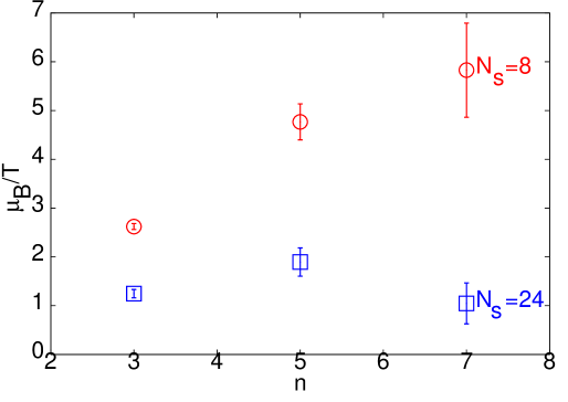
Figure 3: The two estimators of the radius of convergence of the series for $\chi_{20}(\mu_{B})$— (a) $\rho_{2n}$ and (b) $r_{2n}$. The nature of the finite volume effects are clear.

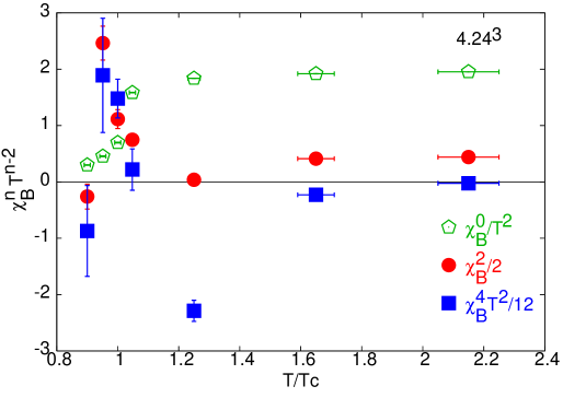
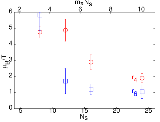
Figure 4: The first panel shows the Taylor coefficients of $\chi_{20}$ at orders 0, 2 and 4 as a function of $T/T_{c}$. The second shows $r_{4}$ and $r_{6}$ at $T=0.95t_{c}$ as a function of $V^{1/3}$ and $\cal V$.

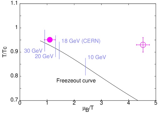
Figure 5: Our evaluation of the critical end point for QCD in the thermodynamic limit compared to an earlier evaluation [7]. Also shown is the freezeout curve in heavy-ion collisions with the center of mass energy marked. It seems that energy scans at RHIC may see interesting physics.

Given the Taylor expansion of an even function $f(x)=\sum_{n}f_{2n}x^{2n}$ around the symmetric point $x=0$, one may define the radius of convergence, $x_{*}$, in several equivalent ways. Two definitions which we use here are the limits of the successive approximants

$$\rho_{2n}=\left|\frac{f_{0}}{f_{2n}}\right|^{1/2n}\quad{\rm or}\quad r_{2n}=\sqrt{\left|\frac{f_{2n}}{f_{2n+2}}\right|}$$ (3)

The results for $\chi_{20}(\mu_{B})$ evaluated on two different volumes are shown in Figure 3 at $T=0.95T_{c}$. Note that the volume effects are compatible with the expectations discussed in Section 1.

One important question is whether the series diverges for real $\mu_{B}$ or imaginary $\mu_{B}$. If it is the first possibility which is realized, then all terms in the series should be positive; if the second, then the series should alternate. We find that all the terms are positive in the range $0.8\leq T/T_{c}\leq 1$, within which the CEP is located (see the first panel of Figure 4), indicating that the first possibility is actually realized. For $N_{f}=2$ the only other nearby critical point is that at $\mu_{I}/T_{c}=m_{\pi}/T_{c}=1.6$ for $T=0$. This is further away from the origin than the critical point identified by the radius of convergence. Hence we conclude that the radius of convergence identifies the CEP.

Finite size effects are of two kinds. At small volumes, i.e., when ${\cal V}<5$ (in this formula the appropriate value of $m_{\pi}$ to use is that measured in very large volumes at $T=0$), the finite volume effects are dominated by the infrared cutoff on the Dirac eigenvalues presented by the volume. Thermodynamics is recovered when ${\cal V}>5$. We show the effects of this crossover in the second panel of Figure 4. In the large volume portion one may use standard (thermodynamic) finite size scaling analysis (using the expected Ising exponents) to continue the results to infinite volume.

Our final result on the CEP are displayed in Figure 5. Also shown for comparison is an older evaluation of this point by a different method in $N_{f}=2+1$ QCD with the same pion mass and a volume ${\cal V}\leq 3.9$ [7] (other approaches include [8, 9, 10, 11]). Since our results at the comparable volumes agree with this evaluation, we believe that the discrepancy cannot be attributed to the difference in the flavour content of the sea. Also shown for comparison is the freezeout curve in heavy-ion collisions. It seems that the CEP may be observed in energy scans at the RHIC.

References

- [1] R. V. Gavai and S. Gupta, Pressure and non-linear susceptibilities in QCD at finite chemical potentials, Phys. Rev. D 68 (2003) 034506, [hep-lat/0303013].
- [2] R. V. Gavai and S. Gupta, On the critical end point of QCD, Phys. Rev. D 71 (2005) 114014 [hep-lat/0412035].
- [3] M. Charikar et al., Approximation algorithms for directed Steiner Tree problems, Stanford University Technical Report STAN-CS-TN-97-56.
- [4] R. V. Gavai and S. Gupta, Simple patterns for non-linear susceptibilities near , Phys. Rev. D (2005) to appear, [hep-lat/0507023].
- [5] C. Bernard et al., QCD thermodynamics with three flavours of improved staggered quarks, Phys. Rev. D 71 (2005) 034504 [hep-lat/0405029].
- [6] R. V. Gavai and S. Gupta, Valence quarks in the QCD plasma, Phys. Rev. D 67 (2003) 034501, [hep-lat/0211015].
- [7] Z. Fodor and S. Katz, Lattice determination of the critical point of QCD at finite and , JHEP 0203 (2002) 014, [hep-lat/0106002].
- [8] M.-P. Lombardo and M. d’Elia, Finite density QCD via imaginary chemical potential, Phys. Rev. D 67 (2003) 014505, [hep-lat/0209146].
- [9] Ph. de Forcrand and O. Philipsen, The QCD phase diagram for small densities from imaginary chemical potential, Nucl. Phys. B 642 (2002) 290, [hep-lat/0205016].
- [10] C. R. Allton et al., The equation of state for two flavour QCD at nonzero chemical potential, Phys. Rev. D 68 (2003) 014507, [hep-lat/0305007].
- [11] V. Azcoiti et al., Phase diagram of QCD with four quark flavours at finite temperature and baryon density, [hep-lat/0503010]