A (P)HMC algorithm for $N_{f}=2+1+1$ flavours of twisted mass fermions

Abstract:

We present a detailed design of a (P)HMC simulation algorithm for $N_{f}=2+1+1$ maximally twisted Wilson quark flavours. The algorithm retains even/odd and mass-shift preconditionings combined with multiple Molecular Dynamics time scales for both the light mass degenerate, $u$ and $d$, quarks and the heavy mass non-degenerate, $s$ and $c$, quarks. Various non-standard aspects of the algorithm are discussed, among which those connected to the use of a polynomial approximation for the inverse (square root of the squared) Dirac matrix in the $s$ and $c$ quark sector.

PoS(LAT2005)103

1 Introduction and motivation

A realistic setup for studying many non-perturbative QCD properties is obtained by introducing two quark pairs, a light ($l$) mass degenerate one ($u$ and $d$ flavours: $2$) and a heavier ($h$) mass non-degenerate one ($s$ and $c$ flavours: $1+1$): for short $N_{f}=2+1+1$. Monte Carlo simulations in this setup are becoming increasingly feasible in the tmLQCD formulation [1, 2, 3] with action

$$S=S_{G}[U]+\bar{\psi}_{l}~{}D_{l}[U]~{}\psi_{l}+\bar{\psi}_{h}~{}D_{h}[U]~{}\psi_{h}~{}~{}~{}~{},~{}~{}~{}~{}\psi_{l}=[u,d]~{}~{}~{}~{},~{}~{}~{}~{}\psi_{h}=[s,c]\;.$$ (1)

Here $S_{G}$ is a suitable pure gauge action , the Dirac operators read (in the “physical” quark basis)

$$D_{l}=\gamma\tilde{\nabla}-i\gamma_{5}\tau_{1}W_{cr}+\mu_{l}\;, \qquad D_{h}=\gamma\tilde{\nabla}-i\gamma_{5}\tau_{1}W_{cr}+\mu_{h}-\epsilon_{h}\tau_{3}\;,$$ (2)

$$W_{cr}=-\frac{a}{2}\nabla^{*}\nabla+M_{cr}\;, M_{cr}=\frac{1}{2\kappa_{cr}}-4\;,$$ (3)

and $\epsilon_{h}$ is the bare $s$–$c$ quark mass splitting. Among the general features of the above formulation [3] we recall: automatic O($a$) improvement [2], robust quark mass protection against “exceptional configurations” [1], expected moderate CPU-cost for unquenched simulations (assuming metastability problems related to the lattice phase structure are solved) [3]. The determinant of $D_{h}$ (eq. (2)) is real and positive provided $|\epsilon_{h}|<|\mu_{h}|$, which, if $Z_{P}/Z_{S}<1$, induces some limitation on the renormalised quark masses, $\hat{m}_{c,s}=Z_{P}^{-1}(\mu_{h}\pm\frac{Z_{P}}{Z_{S}}\epsilon_{h})$, one can simulate.

Through rescaling and chiral rotations of the quark fields (which do not affect the fermion determinant, besides an irrelevant constant factor) and by setting $\tilde{\mu}_{l,h}=2\kappa_{cr}\mu_{l,h}~{},~{}\tilde{\epsilon}_{l,h}=2\kappa_{cr}\epsilon_{l,h}$, the lattice Dirac operators (eq. (2)) can be rewritten in a form more convenient for MC simulations:

$$(\tilde{D}_{l})_{2\times 2}=\left[\gamma\tilde{\nabla}+W_{cr}\right]2\kappa_{cr}+i\tilde{\mu}_{l}\gamma_{5}\tau_{3}\;,\qquad(\tilde{D}_{h})_{2\times 2}=\left[\gamma\tilde{\nabla}+W_{cr}\right]2\kappa_{cr}+i\tilde{\mu}_{h}\gamma_{5}\tau_{3}+\tilde{\epsilon}_{h}\tau_{1}\;.$$ (4)

As the value of $\kappa_{cr}$ is a priori unknown, $\kappa_{cr}$ is generically replaced by $\kappa$ in the definition of $\tilde{\mu}_{l,h}$ and $\tilde{\epsilon}_{l,h}$ . With these premises, we focus on the $\gamma_{5}$-Hermitian partner of the Dirac operator(s) above,

$$\tilde{Q}_{2\times 2}=\left[\begin{array}[]{cc}\tilde{Q}+i\tilde{\mu}&\tilde{\epsilon}\gamma_{5}\\ \tilde{\epsilon}\gamma_{5}&\tilde{Q}-i\tilde{\mu}\end{array}\right]\equiv\left[\begin{array}[]{cc}\tilde{Q}_{+}&\tilde{\epsilon}\gamma_{5}\\ \tilde{\epsilon}\gamma_{5}&\tilde{Q}_{-}\end{array}\right]\;,\qquad\tilde{Q}\equiv\gamma_{5}\left(\gamma\tilde{\nabla}-\frac{a}{2}\nabla^{*}\nabla+\frac{1}{2\kappa}-4\right)2\kappa\;,$$ (9)

where we have for the moment dropped the quark pair labels $l$ and $h$. In the mass degenerate case ($\tilde{\epsilon}=0$), a standard HMC algorithm can be employed in view of

$$\det[\tilde{Q}_{2\times 2}]=\det[\tilde{Q}_{+}\tilde{Q}_{-}]=\det[\tilde{Q}_{cr}^{2}+\mu^{2}]~{}\Leftrightarrow~{}\int\mathcal{D}\phi~{}e^{-\phi^{{\dagger}}(\tilde{Q}_{+}\tilde{Q}_{-})^{-1}\phi}\;,$$

with $\phi$ a single flavour pseudofermion field. This fits well our needs for the $l$ quark pair. In the mass non-degenerate case ($\tilde{\epsilon}\neq 0$) no plain HMC algorithm is straightforwardly applicable because

$$\det[\tilde{Q}_{2\times 2}]=\det[\tilde{Q}_{+}\gamma_{5}\tilde{Q}_{-}-\tilde{\epsilon}^{2}\gamma_{5}]=\det[\tilde{Q}_{+}\tilde{Q}_{-}-\tilde{\epsilon}^{2}\tilde{Q}_{+}\gamma_{5}\tilde{Q}_{+}^{-1}\gamma_{5}]\;,$$ (10)

cannot be reproduced by $\int\mathcal{D}\phi~{}e^{-\phi^{{\dagger}}(AA^{{\dagger}})^{-1}\phi}$, with $A$ a 1-flavour matrix. Owing to the flavour non-diagonal structure of the matrix (9), we propose to deal with a two-flavour matrix, $\tilde{Q}_{2\times 2}\tilde{Q}_{2\times 2}^{{\dagger}}$, acting on a two-flavour pseudofermion field, $\Phi$, and to use a polynomial $P(s)\simeq 1/\sqrt{s}$, which gives

$$\det[\tilde{Q}_{2\times 2}]~{}\Leftrightarrow~{}\int\mathcal{D}\Phi~{}e^{-\Phi^{{\dagger}}(\tilde{Q}_{2\times 2}\tilde{Q}_{2\times 2}^{{\dagger}})^{-1/2}\Phi}~{}\simeq~{}\int\mathcal{D}\Phi~{}e^{-\Phi^{{\dagger}}P(\tilde{Q}_{2\times 2}\tilde{Q}_{2\times 2}^{{\dagger}})\Phi}\;,\qquad\Phi=\left(\begin{array}[]{cc}\phi^{\prime}\\ \phi^{\prime\prime}\end{array}\right)\;,$$ (11)

at least in the $\Phi$-heatbath and the reweighting (or acceptance) correction. A PHMC algorithm [6, 7] appears thus a natural choice to include the effects of the $h$ quark pair in MC simulations.

2 A preconditioned (P)HMC algorithm for $N_{f}=2+1+1$ flavours

We outline here the mixed HMC-PHMC (briefly (P)HMC) algorithm we are developing, which incorporates even-odd (EO) and mass-shift preconditionings [8]. Using different Molecular Dynamics (MD) time steps for different MD force contributions we expect to obtain a good performance, in line with that recently achieved in simulations with two Wilson quark flavours [9, 10].

Denoting by $\Pi$ the momenta conjugated to the gauge field, the MD-Hamiltonian reads

$$H_{2+1+1}\quad = \quad\frac{1}{2}\Pi\cdot\Pi+S_{G}+\Phi^{{\dagger}}_{h}~{}P\left(\hat{Q}_{h}\hat{Q}_{h}^{\dagger}\right)_{h}\Phi_{h}+$$ (12)

$$+ \phi_{1}^{{\dagger}}\left[\hat{Q}_{l}^{\prime}(\hat{Q}_{l}^{\prime})^{\dagger}\right]^{-1}\phi_{1}+\phi_{2}^{{\dagger}}\left\{\hat{Q}_{l}^{\prime}\left[\hat{Q}_{l}^{\prime\prime}(\hat{Q}_{l}^{\prime\prime})^{\dagger}\right]^{-1}(\hat{Q}_{l}^{\prime})^{\dagger}\right\}\phi_{2}\;,$$

where $P(\hat{Q}_{h}\hat{Q}_{h}^{\dagger})$ is a polynomial in $\hat{Q}_{h}\hat{Q}_{h}^{\dagger}$ approximating $[\hat{Q}_{h}\hat{Q}_{h}^{\dagger}]^{-1/2}$ (see sect. 3) while in the $l$ quark sector mass-shift preconditioning is applied [4, 10] on top of EO preconditioning (see eq. (17) and eq. (18)). In this way we need two pseudofermions, $\phi_{1}$ and $\phi_{2}$, for the $l$ quark sector and a two-flavour pseudofermion field, $\Phi_{h}$, for the $h$ quark sector. The EO preconditioned Dirac operators are

$$\hat{Q}_{h}=\gamma_{5}\left[\begin{array}[]{cc}1+i\tilde{\mu}_{h}\gamma_{5}-\frac{M_{oe}(1-i\tilde{\mu}_{h}\gamma_{5})M_{eo}}{1+\tilde{\mu}_{h}^{2}-\tilde{\epsilon}_{h}^{2}}&\tilde{\epsilon}_{h}\left(1+\frac{M_{oe}M_{eo}}{1+\tilde{\mu}_{h}^{2}-\tilde{\epsilon}_{h}^{2}}\right)\\ \tilde{\epsilon}_{h}\left(1+\frac{M_{oe}M_{eo}}{1+\tilde{\mu}_{h}^{2}-\tilde{\epsilon}_{h}^{2}}\right)&1-i\tilde{\mu}_{h}\gamma_{5}-\frac{M_{oe}(1+i\tilde{\mu}_{h}\gamma_{5})M_{eo}}{1+\tilde{\mu}_{h}^{2}-\tilde{\epsilon}_{h}^{2}}\end{array}\right]\;,$$ (15)

$$(M_{eo(oe)})_{x,y}=-\kappa\sum_{\mu}\left[(1+\gamma_{\mu})U^{{\dagger}}_{\mu}(y)\delta_{y,x-\hat{\mu}}+(1-\gamma_{\mu})U_{\mu}(x)\delta_{y,x+\hat{\mu}}\right]\;,$$ (16)

with $\hat{Q}_{h}$ having a $2\times 2$ flavour structure that is made apparent in the r.h.s. of eq. (15), and

$$\hat{Q}_{l}^{\prime} = \gamma_{5}\left[1+i\left(\tilde{\mu}_{l}+\delta\tilde{\mu}_{l}\right)\gamma_{5}-\frac{M_{oe}(1-i\left(\tilde{\mu}_{l}+\delta\tilde{\mu}_{l}\right)\gamma_{5})M_{eo}}{1+\left(\tilde{\mu}_{l}+\delta\tilde{\mu}_{l}\right)^{2}}\right]\;,$$ (17)

$$\hat{Q}_{l}^{\prime\prime} = \gamma_{5}\left[1+i\tilde{\mu}_{l}\gamma_{5}-\frac{M_{oe}(1-i\tilde{\mu}_{l}\gamma_{5})M_{eo}}{1+\tilde{\mu}_{l}^{2}}\right]\;,$$ (18)

with $\hat{Q}_{l}^{\prime}$ and $\hat{Q}_{l}^{\prime\prime}$ carrying the shifted ($\tilde{\mu}_{l}+\delta\tilde{\mu}_{l}$) and the physical ($\tilde{\mu}_{l}$) twisted mass parameters. We remark that (due to the absence of the Sheikholeslami–Wohlert term in the fermionic action) the gauge field enters the Dirac matrices eqs. (15), (17) and (18) only through $M_{eo}$ and $M_{oe}$, eq. (16). It follows that the evaluation of the MD driving force $\dot{\Pi}=-\delta_{U}H_{2+1+1}$ can be, as usual, traced back to that of $\delta_{U}M_{eo}$ and $\delta_{U}M_{oe}$ plus the (many) necessary applications of the relevant Dirac matrices.

With the (P)HMC update [7, 10] dictated by the Hamiltonian $H_{2+1+1}$ (eq. (12)) one ends (after thermalisation) with a sample of gauge configurations equilibrated with respect to the effective gauge action $S_{G}[U]-\log|\det\hat{Q}^{\prime\prime}_{l}|^{2}+\log\det P(\hat{Q}_{h}\hat{Q}_{h}^{\dagger})$. A way to correct for the polynomial approximation of $[\hat{Q}_{h}\hat{Q}_{h}^{\dagger}]^{-1/2}$ is to reweight all the observables ${\cal O}={\cal O}[U]$ with a correction factor [7] that provides a noisy estimate of  $\det[\hat{Q}_{h}\hat{Q}_{h}^{\dagger}]^{1/2}P(\hat{Q}_{h}\hat{Q}_{h}^{\dagger})=\det\hat{Q}_{h}P(\hat{Q}_{h}\hat{Q}_{h}^{\dagger})$ (see also sect. 3).

2.1 MD force contributions and multiple time scales

The MD driving force can be defined (omitting for brevity all indices) as

$$\dot{\Pi}=-\delta_{U}H_{2+1+1}\equiv{\rm tr~{}}\left[\delta UF+F^{{\dagger}}\delta U^{{\dagger}}\right]\;,\qquad F=F_{G}+F_{h}+F_{l1}+F_{l2}\;,$$ (19)

where (see eq. (12)) the pure gauge contribution $(F_{G})$ is completely standard, the $l$ quark sector contributions ($F_{l1}$ and $F_{l2}$) can be straightforwardly evaluated following Refs. [10, 11] and also the $h$ quark sector contribution ($F_{h}$) poses no principle problems (see sect. 3 for more details).

Based on Refs. [9, 10], we expect that for typical choices of $S_{G}$, the lattice spacing and the quark masses, one can have a hierarchy in the average ($av$) size of the individual force contributions,

$$|F_{G}|_{av}~{}>~{}|F_{l1}|_{av}~{}>~{}|F_{l2}|_{av}\;,\qquad|F_{l1}|_{av}~{}\geq~{}|F_{h}|_{av}~{}\geq~{}|F_{l2}|_{av}\;,$$ (20)

provided $\tilde{\mu}_{l}>0$ is not too small and $\delta\tilde{\mu}_{l}>0$ is appropriately chosen [10]. $|F_{h}|_{av}$ is expected to be small for heavy quark masses, i.e. large $|\tilde{\mu}_{h}|$ and $|\tilde{\mu}_{h}|>|\tilde{\epsilon}_{h}|$ .

The hierarchy in eq. (20) –once realised– suggests that an optimal performance is obtained by implementing a MD leapfrog scheme where the force contributions $(F_{G},F_{h},F_{l1},F_{l2})$ enter associated to different time steps $(\delta\tau_{G},\delta\tau_{h},\delta\tau_{l1},\delta\tau_{l2})$ so as to get

$$|F_{G}|_{av}\delta\tau_{G}\simeq|F_{h}|_{av}\delta\tau_{h}\simeq|F_{l1}|_{av}\delta\tau_{l1}\simeq|F_{l2}|_{av}\delta\tau_{l2}\;,\qquad\delta\tau_{i}N_{i}\equiv\tau_{traj}\;,\quad i=\{G,l1,l2,h\}\;,$$ (21)

with $(N_{G},N_{h},N_{l1},N_{l2})$ a set of integers and $\tau_{traj}\sim 1$ the time length of a MD trajectory.

2.2 Some possible algorithmic variants

Several modifications of the above (P)HMC algorithmic scheme are of course possible. For instance, the correction for the polynomial approximation can be moved, fully or partially, from the reweighting to a modified A/R Metropolis step [12, 13]. If this is done “fully” the modified A/R step compensates for both $\det[\sqrt{\hat{Q}_{h}\hat{Q}_{h}^{\dagger}}P(\hat{Q}_{h}\hat{Q}_{h}^{\dagger})]\neq 1$ and the finite MD time step(s).

The update of the gauge field itself can be performed by means of a Multiboson-like algorithm [14] using suitable polynomials to approximate the appropriate power of the inverse Hermitean Dirac matrices (see e.g. Ref. [13] for more details) relevant for the $l$ and $h$ quark sectors.

Another interesting possibility is to employ a non-standard HMC algorithm, whose MD is guided by an Hamiltonian $\tilde{H}\neq H_{2+1+1}$ such that a good acceptance is still obtained in the A/R test. One might try e.g. an $\tilde{H}$ that differs from $H_{2+1+1}$ (eq. (12)) only by the replacement of $\Phi^{{\dagger}}_{h}~{}P(\hat{Q}_{h}\hat{Q}_{h}^{\dagger})_{h}\Phi_{h}$ with $\Phi^{{\dagger}}_{h}~{}\hat{Q}_{h}^{-1}\Phi_{h}$. Numerical experience is of course crucial to test these possible variants and choose the most efficient one.

3 Polynomial approximations for the $h$ quark sector ($s$ and $c$ flavours)

The well known Chebyshev polynomial approximation method allows to approximate the inverse square root of the operator $\hat{S}=\rho_{h}\hat{Q}_{h}\hat{Q}_{h}^{\dagger}$, where $\rho_{h}$ is a positive normalisation factor such that on “practically all” gauge configurations the highest eigenvalue of $\hat{S}$, say $s_{H}$, satisfies $0.8\leq s_{H}<1$. The polynomial $P(\hat{S})=P_{n,s_{L}}(\hat{S})$ of even degree $n$ in $\hat{S}$ that is designed to approximate $\hat{S}^{-1/2}$ in the eigenvalue interval $[s_{L},1]$  can be written (via a product representation with a normalisation factor ${\cal N}>0$ and roots $z_{k}$, $k=1,\dots,n$ such that $z_{n+1-k}=z_{k}^{*}\;$) in a manifestly positive form

$$P_{n,s_{L}}(\hat{S})={\cal N}\prod_{k=1}^{n}(\hat{S}-z_{k})\quad\Rightarrow\quad P_{n,s_{L}}\equiv B_{n/2,s_{L}}B_{n/2,s_{L}}^{\dagger}=\hat{S}^{-1/2}\left[1+R_{n,s_{L}}\right]\;,$$ (22)

where $R_{n,s_{L}}=R_{n,s_{L}}(\hat{S})$ is called the relative fit error. Denoting by $s$ a generic eigenvalue of $\hat{S}$, in Fig. 1 (left panel) we plot for illustration the relative fit error $R_{n,s_{L}}(s)$ for $s_{L}=10^{-4}$ and a value of $n$, namely $n=162$, taken such that $|R_{n,s_{L}}(s)|\leq 0.03$. The chosen value of $s_{L}$ is rather conservative, since it is very low as compared to those that, based on simulation experience with two mass degenerate quarks, we expect to have to face in the $h$ quark sector while working with realistic parameters. We see from Fig. 1 that $R_{n,s_{L}}(s)$ tends to increase when decreasing $s\in[s_{L},1]$, which we believe is acceptable in view of the expected non-high density of eigenvalues in the low end of the spectrum of $\hat{S}$. A conservative and an “effective” measure of the magnitude of the relative fit error are thus given, respectively, by $\delta_{IR}\equiv\max_{s\in[s_{L},1]}|R_{n,s_{L}}(s)|=|R_{n,s_{L}}(s_{L})|$ and $\delta_{UV}\equiv\max_{s\in[0.5,1]}|R_{n,s_{L}}(s)|$ with $\delta_{UV}$ smaller than $\delta_{IR}$ (typically by an order of magnitude).

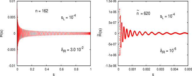
Figure 1: $R(s)=R_{n,s_{L}}(s)$ for $(n,s_{L})=(162,10^{-4})$ (left) and $\tilde{R}(s)=\tilde{R}_{\tilde{n},s_{L}}(s)$ for $(\tilde{n},s_{L})=(620,10^{-4})$ (right).

For the task of computing the contribution $F_{h}$ to the MD driving force we plan to exploit the product representation of $P_{n,s_{L}}(\hat{S})$, see eq. (22), and then proceed analogously to Ref. [7]. A careful ordering [15] of the $n$ monomials in $\hat{S}$ together with 64 bit precision should be sufficient to keep rounding errors under control for polynomials with $n$ up to one thousand.

There are two places where a second polynomial approximation (or an equivalent method such as a rational CG solver [16]) is needed. The first place is the generation of $\Phi_{h}$ distributed according to $\exp[-\Phi_{h}^{\dagger}P_{n,s_{L}}(\hat{S})\Phi_{h}]$, see eq. (12). If $r_{h}$ is a random Gaussian (two flavour) vector, we can construct $\Phi_{h}=B_{n/2,s_{L}}^{-1}(\hat{S})~{}r_{h}~{}$ by e.g. evaluating

$$\Phi_{h}=\tilde{P}_{\tilde{n},s_{L}}(\hat{S})B_{n/2,s_{L}}^{\dagger}(\hat{S})~{}[\sqrt{\rho_{h}}\hat{Q_{h}}]~{}r_{h}\;,\qquad\tilde{P}_{\tilde{n},s_{L}}(\hat{S})=\left[\sqrt{\hat{S}}P_{n,s_{L}}(\hat{S})\right]^{-1}\left[1+\tilde{R}_{\tilde{n},s_{L}}(\hat{S})\right]\;,$$ (23)

where $\tilde{P}_{\tilde{n},s_{L}}(\hat{S})$ is a new polynomial of degree $\tilde{n}$ in $\hat{S}$ that approximates $[\sqrt{\hat{S}}P_{n,s_{L}}(\hat{S})]^{-1}$ with very high precision in the eigenvalue interval $[s_{L},1]$. Values of the corresponding relative fit error, $\tilde{R}_{\tilde{n},s_{L}}$, not exceeding in modulus $\tilde{\delta}_{IR}=10^{-6}$ can be reached for a degree $\tilde{n}=620$, in the above mentioned case of $s_{L}=10^{-4}$ and $n=162$, as it is illustrated in Fig. 1 (right panel). The evaluation of $\tilde{P}_{n,s_{L}}(\hat{S})$ times a vector can be safely performed in 64 bit arithmetics by using a recursive relation (such as Clenshaw’s) that is stable against roundoff.

The other place where the high precision polynomial $\tilde{P}_{n,s_{L}}(\hat{S})$ in eq. (23) may be useful is in the evaluation of $W[\eta;U]=\exp\left\{\eta^{{\dagger}}\left(1-[P_{n,s_{L}}(\hat{S})\sqrt{\hat{S}}]^{-1}\right)\eta\right\}$, the noisy reweighting factor that is needed to get the “exact” v.e.v. of a generic observable ${\cal O}={\cal O}[U]$ (here $\eta$ is the noise field) [7]

$$\langle{\cal O}\rangle=\int D\mu[U]\int D\eta~{}e^{-\eta^{\dagger}\eta}~{}W[\eta;U]~{}{\cal O}[U]\;/\;\int D\mu[U]\int D\eta~{}e^{-\eta^{\dagger}\eta}~{}W[\eta;U]\;,$$

$$\quad\int D\mu[U]\equiv\int DUe^{-S_{G}[U]}~{}\det[\hat{Q}_{l}^{\prime\prime}\hat{Q}_{l}^{\prime\prime{\dagger}}[U]]~{}\det\left[P(\hat{S}[U])\right]^{-1}~{}\equiv~{}Z_{(P)HMC}\quad.$$ (24)

4 Conclusions and Acknowledgements

We discussed an exact algorithm for $N_{f}=2+1+1$ flavours of maximally twisted quarks. Implementation of the algorithm and investigation of important numerical properties, such as the spectrum of $\hat{Q}_{h}\hat{Q}_{h}^{\dagger}$ and the magnitude of the contribution $F_{h}$ to the MD driving force, are in progress.

We thank K. Jansen for many valuable discussions and advises. The work of T. C. is supported by the Deutsche Forschungsgemeinschaft in the form of a Forschungsstipendium CH398/1.

References

- [1] R. Frezzotti et al., Nucl. Phys. Proc. Suppl. 83 941 ; JHEP 0108 058.
- [2] R. Frezzotti and G. C. Rossi, JHEP 0408 007 ; JHEP 0410 070 ; Nucl. Phys. Proc. Suppl. 128 193.
- [3] A. Shindler, these Proceedings ; R. Frezzotti, Nucl. Phys. Proc. Suppl. 140 134.
- [4] F. Farchioni et al., these Proceedings.
- [5] F. Farchioni et al., Eur. Phys. J. C. 42 73.
- [6] P. de Forcrand and T. Takaishi, Nucl. Phys. Proc. Suppl. 53 968.
- [7] R. Frezzotti and K. Jansen, Phys. Lett. B402 328 ; Nucl. Phys. B555 395 and 432.
- [8] M. Hasenbusch, Phys. Lett. B519 177 ; M. Hasenbusch and K. Jansen, Nucl. Phys. B659 299.
- [9] M. Lüscher, hep-lat/0409106 and Refs. therein.
- [10] C. Urbach et al., hep-lat/0506011.
- [11] F. Farchioni et al., Eur. Phys. J. C39 421.
- [12] G. Bhanot and A. D. Kennedy, Phys. Lett. B157 70. A. D. Kennedy and J. Kuti, Phys. Rev. Lett. 54 2473. P. de Forcrand and T. Takaishi, Nucl. Phys. Proc. Suppl. 94 818 and Int. J. Mod. Phys. C13 343.
- [13] I. Montvay and E. Scholz, Phys. Lett. B623 73 and Refs. therein.
- [14] M. Lüscher, Nucl. Phys. B418 637.
- [15] B. Bunk et al., Comput. Phys. Commun. 118 95. I. Montvay, hep-lat/9911014.
- [16] B. Bunk, Nucl. Phys. Proc. Suppl. B63 952.