Abstract

We develop an analytical approach for studying lattice gauge theories within the plaquette representation where the plaquette matrices play the role of the fundamental degrees of freedom. We start from the original Batrouni formulation and show how it can be modified in such a way that each non-abelian Bianchi identity contains only two connectors instead of four. In addition, we include dynamical fermions in the plaquette formulation. Using this representation we construct the low-temperature perturbative expansion for $U(1)$ and $SU(N)$ models and discuss its uniformity in the volume. The final aim of this study is to give a mathematical background for working with non-abelian models in the plaquette formulation.

1 Introduction

1.1 Motivation

There exist several equivalent representations of lattice gauge theories (LGT). Originally, LGT was formulated by K. Wilson in terms of group valued matrices on links as fundamental degrees of freedom [1]. The partition function can be written as

$$Z=\int DU\ \exp\{\beta S[U_{n}(x)]\}\ ,$$ (1)

where $S[U_{n}(x)]$ is some gauge-invariant action whose naive continuum limit coincides with the Yang-Mills action. The integral in (1) is calculated over the Haar measure on the group at every link of the lattice. Very popular in the context of abelian LGT is the dual representation which was constructed in [2]-[4]. Extensions of dual formulations to non-abelian groups have been proposed only in the nineties in [5]-[10]. The resulting dual representation appears to be a local theory of discrete variables which label the irreducible representations of the underlying gauge group and can be written solely in terms of group invariant objects like the $6j$-symbols, etc. A closely related approach to the dual formulation is the so-called plaquette representation invented originally in the continuum theory by M. Halpern [11] and extended to lattice models in [12]. In this representation the plaquette matrices play the role of the dynamical degrees of freedom and satisfy certain constraints expressed through Bianchi identities in every cube of the lattice. Each representation has its own advantages and deficiencies. E.g., the Wilson formulation is well suited for Monte-Carlo simulations, while dual and plaquette representations are usually used for an analytical study of the models. In particular, duals of abelian $U(1)$ LGT have been used to prove the existence of the deconfinement phase transition at zero temperature in four-dimensions ($4D$) [13, 14] and to prove confinement at all couplings in $3D$ [15]. Also Monte-Carlo simulations proved to be very efficient in the dual of $4D$ $U(1)$ LGT [16].

So far, however both dual and plaquette formulations have not been so popular in the case of non-abelian models, probably due to the complexity of these representations. For instance, the plaquette representation can hardly be used for Monte-Carlo computations due to a number of constraints on the plaquette matrices. Let us remind the general form of the Batrouni construction . In [12] the plaquette representation was constructed in the maximal axial gauge. The partition function takes the following form if $S[U_{n}(x)]$ in (1) is the standard Wilson action

$$Z=\int\prod_{p}dV_{p}\exp\left[\beta\sum_{p}{\rm Re\ Tr}V_{p}\right]\prod_{c}J(V_{c})\ ,$$ (2)

where $V_{p}\in SU(N)$ are plaquette matrices, $DV_{p}$ is the invariant Haar measure of $SU(N)$. The product over $c$ runs over all cubes of the lattice. The Jacobian $J(V_{c})$ is given by

$$J(V_{c})=\sum_{r}d_{r}\chi_{r}\left(V_{c}\right)\ ,$$ (3)

where the sum over $r$ is a sum over all representations of $SU(N)$, $d_{r}=\chi_{r}(I)$ is the dimension of the representation $r$. The last expression is nothing but an $SU(N)$ delta-function which introduces certain constraint on the plaquette matrices. This constraint is just the lattice form of the Bianchi identity. The $SU(N)$ character $\chi_{r}$ depends on an ordered product of $SU(N)$ matrices as dictated by the Bianchi identity. Its exact form will be given in the next section. An important point is that in the non-abelian case the resulting constraints on the plaquette matrices appear to be highly-nonlocal and this fact makes an analytical study of the model rather difficult. In particular, it has prevented so far the construction of any well controlled and useful weak-coupling expansion.

A different plaquette formulation of $3D$ $SU(N)$ LGT has been proposed in [17]. It has a local form and does not require gauge fixing. Unfortunately, as we have found by explicit computations the model proposed in [17] does not coincide with the Wilson LGT contrary to the claim of [17]. Exact calculations on a $3^{3}$ lattice show the equivalence between Wilson LGT and the model of [17] but the equivalence is lost already for a $4\times 3^{2}$ lattice. The point is that the constraints on the plaquette matrices in the model of [17] do not match the non-abelian Bianchi identity as will be seen from our explicit calculations. Nevertheless, we have found that a certain decomposition of the lattice made in [17] can be useful in simplifying Batrouni’s original representation. In the next section we use some ideas of [17] to reduce the number of connectors in constraints on plaquette matrices from four to two per each cube of the lattice. This simplifies the whole representation but still it is quite involved.

Let us also mention that there exists a plaquette representation in terms of so-called gauge-invariant plaquettes [18]. This representation does not require gauge fixing and can be formulated both on finite and infinite lattices. It is quite possible to work also with this formulation, all the methods developed in this paper can be straightforwadly extended to the model of gauge-invariant plaquettes. We have nevertheless found that the plaquette formulation obtained in the maximal axial gauge is simpler to handle, especially on finite lattices. Moreover, we shall explain how our formulation can be extended to periodic lattices. In addition to the previous works [12], [17], [18] we include also dynamical fermions in the plaquette formulation.

In spite of the complexity of the plaquette representation, we think it has certain advantages compared to the standard Wilson representation. Some of them have been mentioned and elaborated in [12] and [19]. Duality transformations, Coulomb-gas representation, strong coupling expansion look more natural and simpler in the plaquette formulation. It is also possible to develop a mean-field method which is gauge-invariant by construction and is in better agreement with Monte-Carlo data than any mean-field approach based on the mean-link method [19].

Nevertheless we believe that the main advantage of this formulation, not mentioned in [12], [18] and [19] lies in its applications to the low-temperature region. Let $V_{p}$ be a plaquette matrix in $SU(N)$ LGT. The rigorous result of [20] asserts that the probability $p(\xi)$ that ${\mbox{Tr}}(I-V_{p})\geq\xi$ is bounded by

$$p(\xi)\leq{\cal O}(e^{-b\beta\xi})\ ,\ \beta\to\infty\ ,\ b={\rm{const}}$$ (4)

uniformly in the volume. Thus, all configurations with $\xi\geq O(\beta^{-1})$ are exponentially suppressed. This is equivalent to the statement that the Gibbs measure of $SU(N)$ LGT at large $\beta$ is strongly concentrated around configurations on which $V_{p}\approx I$. This property justifies expansion of the plaquette matrices around unity when $\beta$ is sufficiently large while there is no such justification for the expansion of link matrices, especially in the large volume limit. In particular, we think that replacing ${\rm Tr}V_{p}$ in the Gibbs measure by a Gaussian distribution, in the region of sufficiently large $\beta$ is a well justified approximation. In fact, all the corrections to this approximation must be non-universal.

Actually, this is one of our motivations to construct a low-temperature, i.e. large-$\beta$ expansion of gauge models using the plaquette representation. The well-known problem of the standard perturbation theory (PT), i.e. whether PT is uniformly valid in the volume, can be shortly formulated in the following way. When the volume is fixed, and in the maximal axial gauge the link matrices perform small fluctuations around the unit matrix and the PT works very well producing the asymptotic expansion in inverse powers of $\beta$. However, in the large volume limit the integrand becomes arbitrarily flat even in the maximal axial gauge. It means that in the thermodynamic limit (TL) the system deviates arbitrarily far from the ordered perturbative state, so that no saddle point exists anymore, i.e. configurations of link matrices are distributed uniformly in the group space. That there are problems with the conventional PT was shown in [21], where it was demonstrated that the PT results depend on the boundary conditions (BC) used to reach the TL. Fortunately, even in the TL the plaquette matrices are close to unity, the inequality (4) holds and thus provides a basis for the construction of the low-temperature expansion in a different and mathematically reliable way. In this paper we develop such a weak-coupling expansion both for abelian and non-abelian models.

This paper is organised as follows. In the next section we give our plaquette formulation of $3D$ $SU(N)$ LGT. We work in maximal axial gauge and consider a model with arbitrary local pure gauge action. For fermions we choose either the Wilson or the Kogut-Susskind action. The plaquette representation will be formulated on a dual lattice for the partition function, ’t Hooft and Wilson loops. In section 3 we construct the weak-coupling expansion for the abelian model using the plaquette representation. We give a general expansion for the partition function, calculate the zero-order generating functional and show how to compute corrections and expectation values of Wilson loops. Then, we extend the weak-coupling expansion to an arbitrary $SU(N)$ gauge model. Here we give a general expansion of the Boltzmann factor, explain how to treat the Bianchi constraints in the expansion, compute the generating functional and establish some simple Feynmann rules. Finally, we discuss some features of the large-$\beta$ expansion in non-abelian models. Our conclusions are presented in section 4. Some computations are moved to the Appendices. In Appendix A we study the link Green functions which appear as the main building blocks of the expansion in the plaquette formulation. In the Appendices B and C we give all technical details for the calculation of the free energy expansion for SU(N) models in the plaquette representation.

1.2 Notations and conventions

We work on a $3D$ cubic lattice $\Lambda\in Z^{d}$ with lattice spacing $a=1$, a linear extension $L$ and $\vec{x}=(x,y,z)$, $x,y,z\in[0,L-1]$ denote the sites of the lattice. We impose either free or Dirichlet BC in the third direction and the periodic BC in other directions. Let $G=U(N),SU(N)$; $U_{l}=U_{n}(x)\in G$, $V_{p}\in G$ and $DU_{l}$, $DV_{p}$ denote the Haar measure on $G$. $\chi_{r}(U)$ and $d(r)$ will denote the character and dimension of the irreducible representation $\{r\}$ of $G$, correspondingly. We treat models with local interaction. Let $H[U]$ be a real invariant function on $G$ such that

$$\mid H[U]\mid\ \leq H(I)$$ (5)

for all $U$ and coefficients of the character expansion of $\exp(\beta H)$

$$C[r]\ =\ \int DU\ \exp\left(\beta H[U]\right)\chi_{r}(U)$$ (6)

exist. Introduce the plaquette matrix as

$$V_{p}\>=\>U_{n}(x)U_{m}(x+e_{n})U_{n}^{\dagger}(x+e_{m})U_{m}^{\dagger}(x)\ ,$$ (7)

where $e_{n}$ is a unit vector in the direction $n$. The action of the pure gauge theory is taken as

$$S_{g}[U_{n}(x)]=\sum_{p\in\Lambda}H\left[V_{p}\right]\ .$$ (8)

The action for fermions we write down in the form (colour and spinor indices are suppressed)

$$S_{q}[\overline{\psi}_{f}(x),\psi_{f}(x),U_{n}(x)]=\frac{1}{2}\sum_{x,x^{\prime}\in\Lambda}\sum_{f=1}^{N_{f}}\ \overline{\psi}_{f}(x)A_{f}(x,x^{\prime};U_{l})\psi_{f}(x^{\prime})\ ,$$ (9)

where

$$A_{f}(x,x^{\prime};U_{l})=M_{f}\delta_{x,x^{\prime}}+\frac{1}{2}\sum_{n=1}^{d}\left[\delta_{x+e_{n},x^{\prime}}\xi_{n}(x)U_{n}(x)+\delta_{x-e_{n},x^{\prime}}\overline{\xi}_{n}(x^{\prime})U_{n}^{\dagger}(x^{\prime})\right]\ .$$ (10)

We have introduced here the following notations

$$M_{f}=m_{f}-rd\ ,\ \xi_{n}(x)=r+\gamma_{n}\ ,\ \overline{\xi}_{n}(x)=r-\gamma_{n}$$ (11)

for Wilson fermions and

$$M_{f}=m_{f}\ ,\ \xi_{n}(x)=\overline{\xi}_{n}(x)=\eta_{n}(x)=(-1)^{x_{1}+x_{2}+...+x_{n-1}}$$ (12)

for Kogut-Susskind fermions. $m_{f}$ is mass of the fermion field, $N_{f}$ is the number of quark flavours and $r$ is the Wilson parameter ($r=1$ is a conventional choice).

After integrating out fermion degrees of freedom the partition function of the gauge theory on $\Lambda$ with the symmetry group $G$ can be written as

$$Z_{\Lambda}(\beta,m_{f},N_{f})=\int\prod_{x,n}dU_{n}(x)\times\exp\left\{\beta\sum_{p\in\Lambda}H[V_{p}]+\sum_{f=1}^{N_{f}}{\rm Tr}\ln A_{f}(x,x^{\prime};U_{l})\right\}\ ,$$ (13)

where the trace is taken over space, colour and spinor indices.

2 Plaquette formulation and expression for the Jacobian

In this section we give our formulation of the plaquette representation for $3D$ $SU(N)$ LGT. A short description of our procedure can be found in [22] for pure gauge theory and in [23] for a theory with fermions. In subsection 2.1 we calculate the plaquette representation for the partition function on a dual lattice. In the second subsection we derive the plaquette representation for some observables.

2.1 Expression for the Jacobian

Let us first give a qualitative explanation of our transformations. Consider the partition function given in Eqs. (2) and (3). For the formulation of the Bianchi identity related to a given $3d$-cube we define according to [17] a vertex $A$ in this cube and separated by the diagonal a vertex $B$, see Fig.1. This assignment we extend to all neighbouring cubes and finally to the whole lattice. Thus, all $A$ vertices are separated by 2 lattice spacings, the same is true for $B$ vertices. Next, we take a path connecting the vertices $A$ and $B$ by three links $U_{1}$, $U_{2}$, $U_{3}$ as shown in Fig.1. Then the matrix $V_{c}$ in (2) and (3) entering the Bianchi identity for the cube $c$ can be presented in the following form

$$V_{c}=\left(\prod_{p\in A}V_{p}\right)\ C\left(\prod_{p\in B}V_{p}\right)\ C^{{\dagger}}\ .$$ (14)

$\prod_{p\in A}$ means an appropriately ordered product over three plaquettes of the cube attached to the vertex $A$. The matrix $C$ defines a parallel transport of vertex $A$ into vertex $B$ and equals the product of three link matrices connecting $A$ and $B$, see Fig.1

$$C=U_{1}U_{2}U_{3}^{{\dagger}}\ .$$ (15)

The connector $C$ plays a crucial role in the non-abelian Bianchi identity.

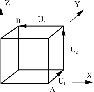
Figure 1: Vertices $A$, $B$ and the connector path on the cube.

Its path has to fit to the choices of $\prod_{p\in A}$ and $\prod_{p\in B}$. We choose the structure of the connectors as shown in Fig.2.

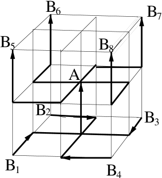
Figure 2: Structure of connectors on the lattice.

This $8$-cube fragment of the lattice is repeated through the whole lattice by simple translation. As is seen from Fig.2 there are only four different types of connectors. For example, the connector $B_{1}A$ is the same as $B_{7}A$. The collection of cubes with the same type of connectors, e.g. $B_{1}A$ form on a dual lattice a body centred cubic (BCC) lattice with double lattice spacing. There are four different sub-lattices of this type corresponding to the four types of connectors in Fig.2: $B_{1}A$, $B_{2}A$, $B_{3}A$ and $B_{4}A$, and therefore four different types of Bianchi identities.

Consider now the partition function given by Eq. (13) on a $3D$ lattice with free or Dirichlet BC in the third direction and periodic BC in other directions for the link matrices. To get the plaquette representation we make a change of variables (7) in the partition function (13). Then the partition function gets the form

$$Z_{\Lambda}(\beta,m_{f},N_{f})=\int\prod_{p}dV_{p}\exp\left\{\beta\sum_{p\in\Lambda}H[V_{p}]\right\}\prod_{p}\ J(V_{p})\ ,$$ (16)

where the Jacobian of the transformation reads

$$J(V_{p})\>=\>\int\prod_{l}dU_{l}\ \prod_{p}\delta\left(V_{p}^{\dagger}\prod_{l\in p}U_{l}-I\right)\exp\left\{\sum_{f=1}^{N_{f}}{\rm Tr}\ln A_{f}(x,x^{\prime};U_{l})\right\}\ .$$ (17)

The last equation is rather formal, for we have to specify the order of multiplications of non-abelian matrices. An important point concerns the position of the plaquette matrix within the product of link matrices. The plaquette matrices $V_{p}$ we insert at the vertices $A$ or $B$ of each plaquette attached to $A$ or $B$, correspondingly. To write down the plaquette delta-functions in (17) explicitly we use the following conventions: 1) a plaquette is always defined as $U_{n}(x)U_{m}(x+e_{n})U_{n}^{\dagger}(x+e_{m})U_{m}^{\dagger}(x)$ with $n<m$, i.e. it starts from the smallest possible coordinate; 2) plaquette matrices are inserted as $V_{p}$, not $V_{p}^{{\dagger}}$ in all vertices $A$ and $B$. Then, for instance, the six delta-functions for the cube $B_{1}A$ in Fig.2 can be written with the notations of Fig.3 as

$$\delta\left(V_{p_{1}}U_{l_{1}}U_{l_{2}}U_{l_{3}}^{{\dagger}}U_{l_{4}}^{{\dagger}}-I\right)\ ,\ \delta\left(V_{p_{2}}U_{l_{1}}U_{l_{5}}U_{l_{9}}^{{\dagger}}U_{l_{8}}^{{\dagger}}-I\right)\ ,\$$

$$\delta\left(V_{p_{3}}U_{l_{4}}U_{l_{7}}U_{l_{12}}^{{\dagger}}U_{l_{8}}^{{\dagger}}-I\right)\ ,\ \delta\left(U_{l_{3}}U_{l_{6}}V_{p_{4}}U_{l_{11}}^{{\dagger}}U_{l_{7}}^{{\dagger}}-I\right)\ ,\$$ (18)

$$\delta\left(U_{l_{2}}U_{l_{6}}V_{p_{5}}U_{l_{10}}^{{\dagger}}U_{l_{5}}^{{\dagger}}-I\right)\ ,\ \delta\left(U_{l_{9}}U_{l_{10}}V_{p_{6}}U_{l_{11}}^{{\dagger}}U_{l_{12}}^{{\dagger}}-I\right)\ .$$

The change of variables in (7) is uniquely determined from these expressions. Similar expressions can be written for all types of connectors using the same rules. Now we want to map one of the plaquette delta’s to a delta-function for the cube using all other delta’s. This procedure can be done for all cubes of the lattice in the following way. We start from the plane $z=L-1$ and use space-like plaquettes (i.e., lying in the $xy$-plane) to map them onto cube delta-function. For the above cube $B_{1}A$ it means that we take the plaquette delta for $V_{p_{6}}$ and substitute link matrices by their expressions obtained from all other delta’s. Then we repeat these calculations for all cubes. One should be careful about the order in which the cubes are taken since to accomplish such calculations for all cubes, the order is important. We can proceed strictly plane by plane and stop at the plane $z=1$. There are still space-like plaquettes left in the plane $z=0$. The connector for a given cube is taken in accordance with Fig.2. Therefore, we mapped all space-like plaquette delta’s lying on the top of a given cube onto cube deltas with connectors lying on the bottom of this cube (in the gauge $U_{3}=I$ defined below). For instance, if the original plaquette lies in the plane $z=z_{i}$, then the connector lies in the plane $z_{i}-1$. These cube delta-functions become samples for the Bianchi constraints. In this way we arrive at the following expression for the Jacobian (17)

$$J(V_{p})\>=\>\int\prod_{l}dU_{l}\ \prod_{p_{0}}\delta\left(V_{p_{0}}^{\dagger}\prod_{l\in p_{0}}U_{l}-I\right)\prod_{i=1}^{4}\prod_{c(i)}J(V_{c}^{(i)})$$

$$\times\exp\left\{\sum_{f=1}^{N_{f}}{\rm Tr}\ln A_{f}(x,x^{\prime};U_{l})\right\}\ ,$$ (19)

where $J(V_{c})$ is given in (3). $\prod_{p_{0}}$ runs over all time-like plaquettes and $\prod_{c(i)}$ means a product over all cubes with the $i$-th type of connector. In the unique notations of Fig.3, the matrices $V_{c}^{(i)}$ for different types of connectors $C_{B_{i}A}$ (see Fig.2) are given by

$$V_{c}^{1}=V_{p_{3}}^{{\dagger}}V_{p_{2}}V_{p_{1}}^{{\dagger}}C_{B_{1}A}V_{p_{5}}V_{p_{6}}V_{p_{4}}^{{\dagger}}C_{B_{1}A}^{{\dagger}}\ ,\ C_{B_{1}A}=U_{l_{4}}U_{l_{3}}U_{l_{6}}\ ,$$ (20)

$$V_{c}^{2}=V_{p_{4}}^{{\dagger}}V_{p_{3}}^{{\dagger}}V_{p_{1}}^{{\dagger}}C_{B_{2}A}V_{p_{2}}V_{p_{6}}V_{p_{5}}C_{B_{2}A}^{{\dagger}}\ ,\ C_{B_{2}A}=U_{l_{3}}U_{l_{2}}^{{\dagger}}U_{l_{5}}\ ,$$ (21)

$$V_{c}^{3}=V_{p_{5}}V_{p_{4}}^{{\dagger}}V_{p_{1}}^{{\dagger}}C_{B_{3}A}V_{p_{3}}^{{\dagger}}V_{p_{6}}V_{p_{2}}C_{B_{3}A}^{{\dagger}}\ ,\ C_{B_{3}A}=U_{l_{2}}^{{\dagger}}U_{l_{1}}^{{\dagger}}U_{l_{8}}\ ,$$ (22)

$$V_{c}^{4}=V_{p_{2}}V_{p_{5}}V_{p_{1}}^{{\dagger}}C_{B_{4}A}V_{p_{4}}^{{\dagger}}V_{p_{6}}V_{p_{3}}^{{\dagger}}C_{B_{4}A}^{{\dagger}}\ ,\ C_{B_{4}A}=U_{l_{1}}^{{\dagger}}U_{l_{4}}U_{l_{7}}\ .$$ (23)

Figure 3: Notations for links and plaquettes of the original cube $B_{1}A$.

The rest of the derivation follows closely Ref.[12]. Choose the maximal axial gauge in the form

$$U_{3}(x,y,z)=U_{2}(x,y,0)=U_{1}(x,0,0)=I\ .$$ (24)

For the Dirichlet BC one has $U_{2}(x,y,0)=U_{1}(x,y,0)=I$. Note, that the gauge fixing procedure and the procedure described above are freely interchangeable. After gauge fixing one can easily obtain expressions for link variables in terms of plaquettes. First of all, space-like links from the plane $z=L-1$ can be trivially integrated out removing all plaquette but Bianchi delta’s from the corresponding cubes near the top boundary of the lattice. Further, we observe that expressions for link variables will depend on the position of a link relatively to the vertex $A$ or $B$. As example, consider a line containing vertices $B$ in $z$ direction, $x,y$ being fixed and let one of the vertices $B$ have the coordinates $B=(x,y,z)$. Then one finds for the link $l=(x,y,z;n_{2})$

$$U_{n_{2}}(x,y,z)=\prod_{z^{\prime}=z-1}^{0}V_{23}(x,y,z^{\prime})\ ,$$ (25)

while for the link $l=(x,y-e_{2},z;n_{2})$

$$U_{n_{2}}(x,y-e_{2},z)=\prod_{z^{\prime}=0}^{z-1}V_{23}(x,y-e_{2},z^{\prime})\ ,$$ (26)

where $V_{23}$ is the plaquette matrix from the $(zy)$-plane. Similar expressions one obtains for all links entering in or coming out of the considered line. Obviously, the same rules apply for links in direction $n_{1}$ as well as for lines containing vertices $A$. Using these expressions one can easily integrate out all link variables in (19). Clearly, the presence of the fermion determinant cannot change the integration procedure. In what follows we pass to the dual lattice where cubes become sites, links become plaquettes and sites become cubes. On the dual lattice our original notations of Fig.3 for the cube $B_{1}A$ become as in Fig.4. This helps us to obtain explicit expressions for the Jacobian.

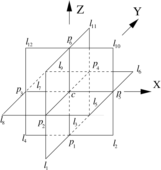
Figure 4: Original cube $B_{1}A$ on the dual lattice.

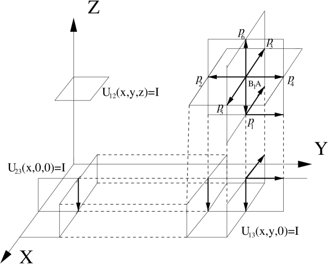
Figure 5: Graphical representation on the dual lattice of the cube delta-function for the cube $B_{1}A$.

Now we can write down the plaquette representation for the $SU(N)$ gauge model on the dual lattice

$$Z_{\Lambda}(\beta,m_{f},N_{f}) = \int\prod_{l}dV_{l}\exp\left[\beta\sum_{l}H[V_{l}]+\sum_{f=1}^{N_{f}}{\rm Tr}\ln A_{f}\left[c(x),c(x^{\prime});U_{l}[V_{l}]\right]\right]$$ (27)

$$\times \prod_{i=1}^{4}\ \prod_{x(i)}\ J\left(V_{x}^{(i)}\right)\ ,$$

where $i=1,2,3,4$ denote four BCC sub-lattices, $\prod_{x(i)}$ runs over all sites of such a BCC sub-lattice and $J(V_{x}^{(i)})$ is an $SU(N)$ delta-function (3). To visualise calculations in the next sections we give here full expressions for the matrices $V_{x}^{(i)}$. As example, we also give the graphical representation of the Bianchi identity for the cube $B_{1}A$ in Fig.5. To write down the full expressions we choose a coordinate system on the dual lattice as shown in Fig.5. Let $\vec{x_{i}}=(x_{i},y_{i},z_{i})$ be a site of the dual lattice which belongs to the $i$-th BCC sub-lattice and introduce notations for dual links

$$l_{1}=(\vec{x_{i}};n_{1})\ ,\ l_{2}=(\vec{x_{i}};n_{2})\ ,\ l_{3}=(\vec{x_{i}};n_{3})\ ,$$

$$l_{4}=(\vec{x_{i}}-e_{1};n_{1})\ ,\ l_{5}=(\vec{x_{i}}-e_{2};n_{2})\ ,\ l_{6}=(\vec{x_{i}}-e_{3};n_{3})\ .$$ (28)

We keep these notations for links attached to any site $x_{i}$. Then, for the type of the connector for the cube $B_{1}A$ one has

$$V_{x}^{(1)}=V_{l_{5}}^{{\dagger}}V_{l_{1}}V_{l_{6}}^{{\dagger}}\ C_{\vec{x}(1)}\ V_{l_{2}}V_{l_{3}}V_{l_{4}}^{{\dagger}}\ C_{\vec{x}(1)}^{{\dagger}}\ ,$$ (29)

$$C_{\vec{x}(1)}=\prod_{k=z_{i}-1}^{1}V_{n_{2}}(x_{i},y_{i}-e_{2},k)\prod_{j=L-1}^{x_{i}}V_{n_{3}}(j,y_{i},0)\prod_{p=1}^{z_{i}-1}V_{n_{1}}(x_{i}-e_{1},y_{i},p)\ ,$$ (30)

for the connector of the cube $B_{2}A$

$$V_{x}^{(2)}=V_{l_{4}}^{{\dagger}}V_{l_{5}}^{{\dagger}}V_{l_{6}}^{{\dagger}}\ C_{\vec{x}(2)}\ V_{l_{1}}V_{l_{3}}V_{l_{2}}\ C_{\vec{x}(2)}^{{\dagger}}\ ,$$ (31)

$$C_{\vec{x}(2)}=\prod_{k=z_{i}-1}^{1}V_{n_{1}}(x_{i}-e_{1},y_{i},k)\prod_{j=x_{i}}^{L-1}V_{n_{3}}(j,y_{i},0)\prod_{p=1}^{z_{i}-1}V_{n_{2}}^{{\dagger}}(x_{i},y_{i},p)\ ,$$ (32)

for the connector of the cube $B_{3}A$

$$V_{x}^{(3)}=V_{l_{2}}V_{l_{4}}^{{\dagger}}V_{l_{6}}^{{\dagger}}\ C_{\vec{x}(3)}\ V_{l_{5}}^{{\dagger}}V_{l_{3}}V_{l_{1}}\ C_{\vec{x}(3)}^{{\dagger}}\ ,$$ (33)

$$C_{\vec{x}(3)}=\prod_{k=z_{i}-1}^{1}V_{n_{2}}^{{\dagger}}(x_{i},y_{i},k)\prod_{j=L-1}^{x_{i}+1}V_{n_{3}}^{{\dagger}}(j,y_{i},0)\prod_{p=1}^{z_{i}-1}V_{n_{1}}^{{\dagger}}(x_{i},y_{i},p)\ ,$$ (34)

and for the connector of the cube $B_{4}A$

$$V_{x}^{(4)}=V_{l_{1}}V_{l_{2}}V_{l_{6}}^{{\dagger}}\ C_{\vec{x}(4)}\ V_{l_{4}}^{{\dagger}}V_{l_{3}}V_{l_{5}}^{{\dagger}}\ C_{\vec{x}(4)}^{{\dagger}}\ ,$$ (35)

$$C_{\vec{x}(4)}=\prod^{1}_{k=z_{i}-1}V_{n_{1}}^{{\dagger}}(x_{i},y_{i},k)\prod_{j=x_{i}+1}^{L-1}V_{n_{3}}^{{\dagger}}(j,y_{i},0)\prod_{p=1}^{z_{i}-1}V_{n_{2}}(x_{i},y_{i}-e_{2},p)\ .$$ (36)

Finally, the fermionic matrix in the gauge (24) can be presented on the dual lattice as

$$A_{f}(c(x),c(x^{\prime});U_{l}[V_{l}])=M_{f}\delta_{c,c^{\prime}}+\frac{1}{2}\left[\delta_{c+e_{3},c^{\prime}}\xi_{3}(c)+\delta_{c-e_{3},c^{\prime}}\overline{\xi}_{3}(c^{\prime})\right]$$

$$+\frac{1}{2}\sum_{n=1}^{2}\left[\delta_{c+e_{n},c^{\prime}}\xi_{n}(c)U_{n}[c;V_{l}]+\delta_{c-e_{n},c^{\prime}}\overline{\xi}_{n}(c^{\prime})U_{n}^{\dagger}[c^{\prime};V_{l}]\right]\ ,$$ (37)

where $c(x)$ is a cube dual to the site $x$. $U_{n}[c;V_{l}]$ is given in (25), (26) for $n=2$ and similar expressions can be easily written for $n=1$.

The expressions for the connectors $C_{\vec{x}(i)}$ in (29)-(36) are given for the free BC. For the Dirichlet BC one should omit the second product $\prod_{j}V_{n_{3}}(j)$ from formulae (30), (32), (34) and (36). Extension of this representation to the lattice with periodic BC in all directions is, at least in principle very simple. Here we give a qualitative explanation only, the details will be given elsewhere. Instead of the maximal axial gauge which is not compatible with the periodic BC one can fix the following gauge

$$U_{3}(x,y,z)=I\ ,\ z\in[1,L-1]\ ;\ U_{3}(x,y,0)=W(\vec{x})=\prod_{z=0}^{L-1}U_{3}(x,y,z)\ ,$$ (38)

where $W$ is the Polyakov line. All the steps performed above are unchanged except for the integration over space-like links in the time slice $z=0$. In this slice the expressions for connectors are modified: they include the values of the Polyakov lines. Therefore, one can express the final result in terms of plaquettes and these Polyakov lines (38).

2.2 Observables on the dual lattice

In this subsection we derive on the dual lattice a representation for the t’ Hooft line and the Wilson loop.

We consider first a t’ Hooft line which in $3D$ consists of a string $S_{xy}$ of dual links between the sites $x$ and $y$ on the dual lattice. For simplicity let us restrict ourselves to pure gauge theory with the Wilson action. With the set $T$ of plaquettes dual to the string $S_{xy}$ we define the action

$$S_{z}(U;T)=\beta\sum_{p\notin T}{\rm ReTr}U_{p}+\beta\sum_{p\in T}{\rm ReTr}zU_{p}$$ (39)

and the partition function

$$Z(z;S_{xy})=\int DU\ \exp\{\beta S_{z}(U;T)\}\ ,$$ (40)

where $z$ is center element of $SU(N)$. We can introduce the disorder operator as

$$\langle D_{z}(S_{xy})\rangle=\frac{Z(z;S_{xy})}{Z(1;S_{xy})}\ .$$ (41)

On the dual lattice the partition function $Z(z,S_{xy})$ of pure gauge theory can be written in the form of Eq.(27) with the action

$$S_{z}(V;S_{xy})=\beta\sum_{l\notin S_{xy}}{\rm ReTr}V_{l}+\beta\sum_{l\in S_{xy}}{\rm ReTr}zV_{l}\ .$$ (42)

Suppose that the points $x$ and $y$ belong to the BCC sub-lattice with the $i=1$ type of connector. By a change of variables $V_{l}\to z^{*}V_{l}$ for $l\in S_{xy}$ we get the following representation for the partition function $Z(z;S_{xy})$

$$Z(z;S_{xy})=\int\prod_{l}dV_{l}\exp\left[\beta\sum_{l}{\rm Re\ Tr}V_{l}\right]\ \prod_{i=1}^{3}\ \prod_{x(i)}\ J\left(V_{x}^{(i)}\right)$$

$$\times\left[\prod_{x(1)\neq x,y}\ J\left(V_{x}^{(1)}\right)\right]\ J\left(zV_{x}^{(1)}\right)J\left(zV_{y}^{(1)}\right)\ ,$$ (43)

since $z$ cancels from all Bianchi constraints but those for the endpoints. Therefore, one can say that the Bianchi constraint is violated at these endpoints. For example, for the $SU(2)$ gauge group $z=-1$ and $J(zV)$ has the form

$$J(zV)=\delta(V+I)=\sum_{r}(-1)^{2r}d_{r}\chi_{r}\left(V\right)\ .$$ (44)

This delta-function constrains the product of non-abelian matrices to $-I$.

Now we give a dual expression for a Wilson loop of size $R\times T$ in some representation $j$. Suppose, for simplicity that the loop contour lies in the $y-z$ plane and $R$, $T$ are even. Generelizing the consideration of the previous subsection it is straightforward to show that such a Wilson loop has the following dual form

$$W_{j}(C)=\langle\ {\rm Tr}_{j}\ \prod_{n=0}^{R/2-1}\left(\prod_{z_{1}=z-1}^{0}V_{1}(x,y+2n,z_{1})\prod_{z_{2}=0}^{z-1}V_{1}(x,y+2n+1,z_{2})\right)$$

$$\prod_{n=R/2-1}^{0}\left(\prod_{z_{1}=0}^{z+T-1}V_{1}^{{\dagger}}(x,y+2n+1,z_{1})\prod_{z_{2}=z+T-1}^{0}V_{1}^{{\dagger}}(x,y+2n,z_{2})\right)\ \rangle\ .$$ (45)

As one can see, the connectors are not cancelled in the general from the Wilson loop. One can simplify this expression taking one side of the loop in the plane $z=0$. Then the Wilson loop is an ordered product of dual links which all lay inside the area spanned by the loop $C$, i.e. the first line in the last formula is unity.

3 Low-temperature expansion

This section is devoted to the construction of the low-temperature expansion of gauge models in the plaquette formulation. In doing this we follow the strategy developed for the two-dimensional principal chiral models in [24]. In that paper a low-temperature expansion was constructed for $SU(N)$ spin models in the link formulation. This formulation appears to be closely related to the plaquette formulation of $3D$ gauge models. For example, as was shown in [12] and [25] in both cases the strong coupling expansion is the expansion towards restoration of the Bianchi identity. As will be seen below, the weak-coupling expansion in both models also bears many common features. In the abelian case they turn out to be practically identical, while the only (but essential) difference in the non-abelian gauge models is the appearance of connectors.

A lattice PT in the maximal axial gauge was constructed for abelian and non-abelian models in the standard Wilson formulation by F. Müller and W. Rühl in [26]. In this gauge the PT for non-abelian models displays serious infrared divergences in separate terms of the expansion starting from ${\cal O}(\beta^{-2})$ order for the Wilson loop and from ${\cal O}(\beta^{-1})$ for the free energy. Of course, it is expected that all divergences must cancel in all gauge invariant quantities. In [26] the authors worked out a special procedure of how to deal with such divergences. The essential ingredients of the procedure of [26] are the following: 1) fixing the Dirichlet BC in one direction and the periodic ones in other directions; 2) a Wilson loop under consideration is placed at distance $R$ from the boundary and the limit $R\to\infty$ is imposed to restore time translation invariance; 3) divergent Green functions must be properly regularised, though there is no a priori preference to any regularization. With this procedure the first two coefficients of the expansion of Wilson loop expectation values in $SU(2)$ LGT have been computed. These coefficients appear to be infrared finite in all $D\geq 3$ and are proportional to the perimeter of the loop in $4D$ and to $R\ln T+T\ln R$ in $3D$ (for a rectangular loop $R\times T$).

We are not aware of any proof of the infrared finiteness at higher orders of the expansion. That there could be a problem with the infrared behaviour was shown however in [21]. Namely, in the addition to the Dirichlet BC on the boundary, one link was fixed in the middle of the lattice and it was shown that the TL value of the expectation value of the plaquette to which the fixed link belong differs from that obtained in [26]. The underlying reason of such infrared behaviour lies, of course in the fact that the conventional PT is done around the vacuum $U_{n}(x)=I$ which is the true ground state only at fixed $L$, even in the maximal axial gauge. When the volume grows the fluctuations of the link matrices become larger and larger and may cause an infrared unstable behaviour. In particular, the integration regions over fluctuations are usually extended to infinity. But only for fixed $L$ one can really prove that this introduces exponentially small corrections. There is no tool for proving that they remain exponentially small also in the large volume limit. On the contrary, bounds on the large plaquette fluctuations (4) holds uniformly in the volume implying that large plaquette fluctuations remain exponentially small also in the TL. This is the first achievement of the low-temperature expansion in the plaquette formulation. Constructing the low-temperature expansion in the plaquette formulation we aim not only to develop a new technics of calculation of the asymptotic expansions in LGT but also to get a deeper insight into this infrared problem and as a consequence into the problem of the uniformity of the low-temperature expansion. We hope that this will help in the investigation of the general properties of asymptotic expansions of non-abelian gauge models. As will be seen below, all Green functions appearing in the plaquette formulation are infrared finite. The source of trouble are the connectors of the non-abelian Bianchi identity. The low-temperature expansion in the plaquette formulation starts from the abelian Bianchi identity (zero order partition function) for every cube and goes towards gradual restoration of the full identity with every order of the expansion. Thus, the generating functional contains an abelianized form of the identity without connectors. High-order terms include expansion of connectors (of course, together with other contributions which are however infrared finite) which can lead to the infrared problem. Let us also mention that in this respect there is a big difference between gauge models and $2D$ $SU(N)$ spin models. In the latter the low-temperature expansion also goes towards restoration of the full non-abelian Bianchi identity [24] and the form of the generating functional is formally the same. It includes invariant link Green functions and the standard Green function. In $2D$ the latter is not infrared finite and is the main source of the trouble. As will be seen below, in $3D$ gauge models all Green functions entering the generating functional are infrared finite. The source of the infrared problem in gauge models are the connectors of the non-abelian Bianchi identities.

3.1 $U(1)$ LGT

For a simple introduction to our method we first consider the abelian $U(1)$ LGT without fermions where the expansion can be done in a straightforward manner. Due to a cancellation of the connectors from Bianchi identities for abelian models the plaquette formulation for the $U(1)$ model on the dual lattice with the Wilson action reads

$$Z_{U(1)}(\beta)=\int_{-\pi}^{\pi}\prod_{l}\frac{d\omega_{l}}{2\pi}\exp\left[\beta\sum_{l}\cos\omega_{l}\right]\prod_{x}J_{x}\ ,$$ (46)

where the Jacobian is given by the periodic delta-function

$$J_{x} = \sum_{r=-\infty}^{\infty}e^{ir\omega_{x}}\ ,$$ (47)

$$\omega_{x} = \omega_{n_{1}}(x)+\omega_{n_{2}}(x)+\omega_{n_{3}}(x)-\omega_{n_{1}}(x-e_{1})-\omega_{n_{2}}(x-e_{2})-\omega_{n_{3}}(x-e_{3})\ .$$

Dual links are defined by the point $x$ and the positive direction $n$, see Eq.(28). Strictly speaking, if the original link gauge matrices satisfy free boundary conditions, and so do the plaquette matrices then the dual links $\omega_{l}$ and representations $r_{x}$ must obey zero Dirichlet BC. All general expansions given below are valid for any type of BC, the dependence on the BC enters only the Green functions defined below. In $3D$ the difference between Green functions for different types of BC is of the order ${\cal O}(L^{-2})$ for large $L$. Since we are interested in the TL behaviour only, we can consider dual models without any reference to the original link representation and introduce any type of BC. Both in abelian and in non-abelian cases we work with periodic BC. We remind at this point that expressions obtained below on a finite lattice do not correspond to the standard link formulation since the latter would include contributions from nontrivial Polyakov loops on a periodic finite lattice. However, in the TL both models must coincide and convergence to the TL is very fast, like ${\cal O}(L^{-2})$. If one wants to recover the exact correspondence between our dual representation and the link representation on the finite lattice with free BC, the only change is that one should take the corresponding Green functions entering the generating functionals.

The construction of the PT proceeds as follows. The first step is a standard one, i.e. we re-scale $\omega\to\omega/\sqrt{\beta}$ and expand the Boltzmann factor in powers of $1/\beta$ as

$$\exp\left[\beta\cos\frac{\omega_{l}}{\sqrt{\beta}}\right]=\exp\left[\beta-\frac{1}{2}(\omega_{l})^{2}\right]\left[1+\sum_{k=1}^{\infty}(\beta)^{-k}A_{k}(\omega_{l}^{2})\right]\ ,$$ (48)

where $A_{k}$ are known coefficients (see, e.g. [24]). Introducing sources $h_{l}$ for the link field, we find

$$Z_{U(1)}(\beta>>1)=e^{3\beta L^{3}-L^{3}\ln\beta}\prod_{l}\left[1+\sum_{k=1}^{\infty}\frac{1}{\beta^{k}}A_{k}\left(\frac{\partial^{2}}{\partial h_{l}^{2}}\right)\right]M_{U(1)}(h_{l})\ ,$$ (49)

where $M_{U(1)}(h_{l})$ is a zero-order generating functional. Using the Poisson summation formula $M_{U(1)}(h_{l})$ can be represented as

$$M_{U(1)}(h_{l})=\sum_{m_{x}=-\infty}^{\infty}\int_{-\infty}^{\infty}\prod_{x}dr_{x}\int_{-\pi\sqrt{\beta}}^{\pi\sqrt{\beta}}\prod_{l}\frac{d\omega_{l}}{2\pi}$$

$$\times\exp\left[-\frac{1}{2}\sum_{l}\omega_{l}^{2}+i\sum_{l}\omega_{l}(r_{x}-r_{x+e_{n}})+2\pi i\sqrt{\beta}\sum_{x}r_{x}m_{x}+\sum_{l}\omega_{l}h_{l}\right]\ .$$ (50)

In addition to the above perturbation one has to extend the integration region over dual link angles $\omega_{l}$ to infinity. Clearly, all the corrections from this perturbation go down exponentially with $\beta$ (it is obvious from the expression for the generating functional, Eq.(50)). Calculating all the integrals in (50) we find up to a constant (sum over all repeating indices is understood)

$$M_{U(1)}(h_{l})=e^{\frac{1}{4}h_{l}G_{ll^{\prime}}h_{l^{\prime}}}\sum_{m_{x}}e^{-\pi^{2}\beta m_{x}G_{x,x^{\prime}}m_{x^{\prime}}+\pi\sqrt{\beta}h_{l}D_{l}(x^{\prime})m_{x^{\prime}}}\ ,$$ (51)

where we have introduced the link Green functions $G_{ll^{\prime}}$ and $D_{l}(x)$ (see Appendix A). $G_{x,x^{\prime}}$ is the Green function of free massless scalar field in $3D$. Up to the first exponent, the generating functional coincides with the dual partition function of the $U(1)$ Villain model in the Coulomb gas representation. From here it follows: Only the configuration $m_{x}=0$ for all $x$ contributes to the asymptotic expansion and non-trivial monopole configurations are exponentially suppressed. We thus get

$$M_{U(1)}(h_{l})=\exp\left[\frac{1}{4}\sum_{l,l^{\prime}}h_{l}G_{ll^{\prime}}h_{l^{\prime}}\right]\ +{\cal O}(e^{-\beta})\ .$$ (52)

Substitution of the last equation into (49) generates a weak-coupling expansion in inverse powers of $\beta$.

The easiest way to construct the corresponding expansion for the Wilson loop is the following. Let $S_{xy}^{d}$ be some surface dual to the surface $S_{xy}$ which is bounded by the loop $C$ and consists of links dual to plaquettes of the original lattice. Let $b$ denote links from $S_{xy}^{d}$. Then, the Wilson loop in representation $J$ is defined as

$$W(C)=\langle\prod_{b\in S^{d}_{xy}}\exp\left[\frac{i}{\sqrt{\beta}}J\omega_{b}\right]\rangle\ .$$ (53)

The last formula suggests that for the computation of the Wilson loop it is sufficient to make the shift $h_{l}\to h_{l}+(i/\sqrt{\beta})J\sum_{b}\delta_{l,b}$ in the expression for the generating functional (52). We find

$$W(C)=\exp\left[-\frac{J^{2}}{4\beta}\sum_{b,b^{\prime}\in S^{d}_{xy}}G_{bb^{\prime}}\right]Z^{-1}_{U(1)}\prod_{l}\left[1+\sum_{k=1}^{\infty}\frac{1}{\beta^{k}}A_{k}\left(\frac{\partial^{2}}{\partial h_{l}^{2}}\right)\right]$$

$$\exp\left[\frac{1}{4}\sum_{l,l^{\prime}}h_{l}G_{ll^{\prime}}h_{l^{\prime}}+\frac{i}{2\sqrt{\beta}}Jh_{l}\sum_{b}G_{lb}\right]\ .$$ (54)

It is now straightforward to calculate all connected pieces contributing to the Wilson loop at a given order of $1/\beta$. For the first coefficients we get

$$W(C)=\exp\left[-\frac{J^{2}}{2\beta}\left(1+\frac{1}{4\beta}\right)P(C)+{\cal O}\left(\beta^{-3}\right)\right]\ ,$$ (55)

where

$$2P(C)=\sum_{b,b^{\prime}\in S^{d}_{xy}}G_{bb^{\prime}}\ .$$ (56)

Using some properties of $G_{ll^{\prime}}$ described in the Appendix A it is easy to prove that this result coincides with the result given in [26] for the $U(1)$ model and for $J=1$. The asymptotic behaviour of $P(C)$ is given by Eq. (93).

3.2 $SU(2)$ LGT

In this subsection we derive the low-temperature expansion for non-abelian models. Again, the general procedure is precisely the same as in $2D$ non-abelian spin models, therefore for some technical details we refer the reader to paper [24]. First, we describe the general procedure for pure $SU(2)$ LGT and then give a simple generalisation for all $SU(N)$ models and include dynamical fermions. For simplicity we work in what follows with the Wilson action, i.e. $H[V_{l}]={\rm Re\ Tr}V_{l}$.

We want to expand the partition and correlation functions into an asymptotic series whose coefficients $\langle B_{k}\rangle_{G}$ are calculated in some ensemble $G$ with a Gaussian measure. For the partition function we expect up to a constant factor an expression of the form

$$Z=1+\sum_{k=1}^{\infty}\frac{1}{\beta^{k}}\langle B_{k}\rangle_{G}\ .$$ (57)

Let us consider the standard parameterisation for the $SU(2)$ link matrix

$$V_{l}=\exp[i\sigma^{k}\omega_{k}(l)]\ ,$$ (58)

where $\sigma^{k},k=1,2,3$ are Pauli matrices and introduce

$$W_{l}=\left[\sum_{k}\omega^{2}_{k}(l)\right]^{1/2}\ \ ,\ W_{x}=\left[\sum_{k}\omega^{2}_{k}(x)\right]^{1/2},$$ (59)

where $\omega_{k}(x)$ is a site angle defined as

$$V_{x}=\exp\left[i\sigma^{k}\omega_{k}(x)\right]=\left(\prod_{p\in A}V_{p}\right)\ C\left(\prod_{p\in B}V_{p}\right)\ C^{{\dagger}}\ .$$ (60)

Here, the site $x$ is dual to the cube $c$ with vertices $A$ and $B$. $\omega_{k}(x)$ has the following expansion in powers of link angles

$$\omega_{k}(x)=\omega^{(0)}_{k}(x)+\omega^{(1)}_{k}(x)+\omega^{(2)}_{k}(x)+\cdots\ .$$ (61)

On the dual lattice (we keep notations (28) for dual links) the first coefficient can be written down as

$$\omega^{(0)}_{k}(x)=\omega_{k}(l_{4})+\omega_{k}(l_{5})+\omega_{k}(l_{6})-\omega_{k}(l_{1})-\omega_{k}(l_{2})-\omega_{k}(l_{3})\ .$$ (62)

$\omega^{(i)}_{k}(x)$ for $i\geq 1$ can be computed by making repeated use of the Campbell-Baker-Hausdorff formula. Then, the partition function (27) can be exactly rewritten to the following form (see Appendix A in the e-print version of [24])

$$Z_{SU(2)}=\int\prod_{l}\left[\frac{\sin^{2}W_{l}}{W^{2}_{l}}\prod_{k}d\omega_{k}(l)\right]\exp\left[2\beta\sum_{l}\cos W_{l}\right]\prod_{x}\frac{W_{x}}{\sin W_{x}}$$

$$\prod_{x}\sum_{m(x)=-\infty}^{\infty}\int\prod_{k}d\alpha_{k}(x)\exp\left[-i\sum_{k}\alpha_{k}(x)\omega_{k}(x)+2\pi im(x)\alpha(x)\right]\ ,$$ (63)

where $\alpha(x)=(\sum_{k}\alpha^{2}_{k}(x))^{1/2}$. For the derivation of this representation we have used the Poisson resummation formula. In order to perform the weak coupling expansion we make the substitution

$$\omega_{k}(l)\to(2\beta)^{-1/2}\omega_{k}(l)\ ,\ \alpha_{k}(x)\to(2\beta)^{1/2}\alpha_{k}(x)$$ (64)

and then expand the integrand of (63) in powers of fluctuations of the link fields. We introduce now the external sources $h_{k}(l)$ coupled to the link field $\omega_{k}(l)$ and $s_{k}(x)$ coupled to the auxiliary field $\alpha_{k}(x)$ and adopt the definitions

$$\omega_{k}(l)\to\frac{\partial}{\partial h_{k}(l)}\ ,\ \alpha_{k}(x)\to\frac{\partial}{\partial s_{k}(x)}\ .$$ (65)

With this convention we get the following expansion for the partition function (63)

$$Z=\left[1+\sum_{k=1}^{\infty}\frac{1}{\beta^{k}}B_{k}\left(\partial_{h},\partial_{s}\right)\right]M(h,s)\ ,$$ (66)

where the operators $B_{k}$ are defined through

$$1 + \sum_{k=1}^{\infty}\frac{1}{\beta^{k}}B_{k}\left(\partial_{h},\partial_{s}\right)=\prod_{x}\left[1+\sum_{q=1}^{\infty}\frac{(-i)^{q}}{q!}\left(\sum_{k}\alpha_{k}(x)\sum_{n=1}^{\infty}\frac{\omega^{(n)}_{k}(x)}{(2\beta)^{n/2}}\right)^{q}\right]$$ (67)

$$\times \prod_{l}\left[\left(1+\sum_{k=1}^{\infty}\frac{1}{(2\beta)^{k}}\sum_{l_{1},..,l_{k}}^{\prime}\frac{a_{1}^{l_{1}}...a_{k}^{l_{k}}}{l_{1}!...l_{k}!}\right)\left(1+\sum_{k=1}^{\infty}\frac{(-1)^{k}}{(2\beta)^{k}}C_{k}W_{l}^{2k}\right)\right]\ .$$

Here we have denoted

$$a_{k}=(-1)^{k+1}\frac{W_{l}^{2(k+1)}}{(2k+2)!}\ ,\ C_{k}=\sum_{n=0}^{k}\frac{1}{(2n+1)!(2k-2n+1)!}\ .$$ (68)

The first brackets on the rhs in Eq.(67) represent the expansion of the Jacobian. The first and the second brackets in the second line come from the expansion of the action and of the invariant measure, correspondingly. We have omitted the expansion of the term $W_{x}/\sin W_{x}$ since it does not contribute to the asymptotic expansion (due to the constraint $W_{x}=0$) but only to exponentially small corrections. As usual, one has to put $h_{k}=s_{k}=0$ after taking all the derivatives. Note, that in writing down these general expansions we do not distinguish between four BCC sub-lattices since the generating functional (see just below) has a unique form for all lattice. Thus, the product over $x$ in Eq.(67) goes over all sites of the dual lattice. The difference between BCC sub-lattices appears only in the general expressions for coefficients $\omega^{(i)}_{k}(x)$ for $i\geq 1$.

The generating functional $M(h,s)$ is given by

$$M(h,s)=\int_{-\infty}^{\infty}\prod_{x,k}d\alpha_{k}(x)\int_{-\infty}^{\infty}\prod_{l,k}d\omega_{k}(l)\exp[-\frac{1}{2}\omega^{2}_{k}(l)-i\omega_{k}(l)[\alpha_{k}(x+e_{n})-\alpha_{k}(x)]]$$

$$\times\ \sum_{m(x)=-\infty}^{\infty}\exp\left[2\pi i\sqrt{2\beta}\sum_{x}m(x)\alpha(x)+\sum_{l,k}\omega_{k}(l)h_{k}(l)+\sum_{x,k}\alpha_{k}(x)s_{k}(x)\right]\ ,$$ (69)

where we extended the integration region for the link angles $\omega_{k}(l)$ to the real axes. As in the abelian case, only the configuration with $m_{x}=0$ for all $x$ contributes to the asymptotic expansion, all others are exponentially suppressed. Calculating all Gaussian integrals in (69) we come to

$$M(h,s)=\exp\left[\frac{1}{4}s_{k}(x)G_{x,x^{\prime}}s_{k}(x^{\prime})+\frac{i}{2}s_{k}(x)D_{l}(x)h_{k}(l)+\frac{1}{4}h_{k}(l)G_{ll^{\prime}}h_{k}(l^{\prime})\right]\ .$$ (70)

From the last expression one can deduce the following simple rules

$$\langle\omega_{k}(l)\omega_{n}(l^{\prime})\rangle=\frac{\delta_{kn}}{2}G_{ll^{\prime}}\ ,\ \langle\alpha_{k}(x)\alpha_{n}(x^{\prime})\rangle=\frac{\delta_{kn}}{2}G_{xx^{\prime}}\ ,-i\langle\omega_{k}(l)\alpha_{n}(x^{\prime})\rangle=\frac{\delta_{kn}}{2}D_{l}(x^{\prime})\ .$$ (71)

The expansion (66), the representation (70) for the generating functional and the rules (71) are the main formulae of this section which allow to calculate the weak coupling expansion of both the free energy and any fixed-distance observable. The extension of this expansion for the Wilson loop is straightforward. Since all gauge invariant quantities depend only on the dual link variables but not on auxiliary fields one can make their direct expansion in powers of link angles.

3.3 $SU(N)$ LGT and dynamical fermions

A generalisation for an arbitrary $SU(N)$ model can be done again precisely like in $2D$ spin models. For completeness, we repeat the arguments of [24] below. It is seen from the procedure outlined above that the low-temperature expansion arises only from the “vacuum” sector with $m_{x}=0$ for all $x$. It follows from Eq.(63) that in this sector the $SU(N)$ delta-function reduces to the Dirac delta-function so that the partition function becomes

$$Z(\beta)=\int\prod_{l}dV_{l}\exp\left[\beta\sum_{l}{\mbox{Re Tr}}V_{l}\right]\int_{-\infty}^{\infty}\prod_{x}\prod_{k=1}^{N^{2}-1}d\alpha_{k}(x)\exp\left[-i\alpha_{k}(x)\omega_{k}(x)\right]\ .$$ (72)

After this simple observation the expansion itself is done precisely like for $SU(2)$.

To include fermions in the above expansion one can proceed in a standard way. Namely, we expand gauge matrices entering the fermionic matrix (37) as

$$U_{n}(c)=\exp[it_{k}\omega_{k}(c,n)]=\sum_{m=0}\frac{i^{m}}{m!}[t_{k}\omega_{k}(c,n)]^{m}\ .$$ (73)

Here $\omega_{k}(c,n)=\omega_{k}(p)$ can be calculated from equations (25) and (26) with the help of the Campbell-Baker-Hausdorf formula. We introduce now the following matrices

$$\hat{G}_{f}^{-1}(c(x),c(x^{\prime}))=M_{f}\delta_{c,c^{\prime}}+\frac{1}{2}\sum_{n=1}^{3}\left[\delta_{c+e_{n},c^{\prime}}\xi_{n}(c)+\delta_{c-e_{n},c^{\prime}}\overline{\xi}_{n}(c^{\prime})\right]$$ (74)

and

$$F(c(x),c(x^{\prime});U_{l}[V_{l}])=\sum_{m=1}\frac{i^{m}}{m!}\sum_{k_{1}...k_{m}}F^{(m)}(c(x),c(x^{\prime}))t_{k_{1}}...t_{k_{m}}\ ,$$ (75)

where

$$F^{(m)}(c(x),c(x^{\prime})) = \frac{1}{2}\sum_{n=1}^{2}[\delta_{c+e_{n},c^{\prime}}\xi_{n}(c)\omega_{k_{1}}(c,n)...\omega_{k_{m}}(c,n)$$ (76)

$$+ (-1)^{m}\delta_{c-e_{n},c^{\prime}}\overline{\xi}_{n}(c^{\prime})\omega_{k_{1}}(c^{\prime},n)...\omega_{k_{m}}(c^{\prime},n)]\ .$$

Then, the fermionic part of the partition function (27) is expanded as

$$\exp\left[\sum_{f=1}^{N_{f}}{\rm Tr}\ln A_{f}\left[c(x),c(x^{\prime});U_{l}[V_{l}]\right]\right]=\prod_{f=1}^{N_{f}}{\rm Det}[\hat{G}_{f}^{-1}]$$

$$\times\exp\left[\sum_{f=1}^{N_{f}}\sum_{s=1}^{\infty}\frac{(-1)^{s}}{s}{\rm Tr}(\hat{G}_{f}F)^{s}\right]\ .$$ (77)

With the substitution (64) and expressing the plaquette angles $\omega_{k}(c,n)$ in terms of $\omega_{k}(l)$ the last formula can be expanded further in powers of fluctuations of dual link variables. This procedure obviously does not change the generating functional therefore all expectation values can be obtained again by differentiating the functional (70).

In order to show how our expansion works in practice we have computed the simplest possible quantity, namely the first order coefficient in the expansion of the free energy. All details of these calculations for $SU(N)$ model are given in the Appendix C.

3.4 Some remarks on the low-temperature expansion

We close this section with brief comments on general properties of the weak coupling expansion in non-abelian models. Consider the zero order partition function. As follows from Eqs.(50) and (72) for the $SU(N)$ group it has the form

$$Z_{G}=\int_{-\infty}^{\infty}\prod_{l,k}d\omega_{k}(l)\exp\left[-\frac{1}{2}\sum_{l,k}\omega_{k}^{2}(l)\right]\prod_{x,k}\delta\left[\omega_{k}^{(0)}(x)\right]\ ,\ k=1,\cdots,N^{2}-1\ .$$ (78)

The integrations are performed over the real axes though originally they are restricted to a compact domain, e.g. for $SU(2)$ to (after change of variables (64)) $\sum_{k}\omega_{k}^{2}(l)\leq\pi^{2}\beta$. From here it follows that the probability for $K$ links to have large fluctuations like $\omega_{k}(l)\sim{\cal O}(\sqrt{\beta})$ is suppressed as ${\cal O}(e^{-{\rm const}K\pi^{2}\beta})$. This is of course only a rough estimate, nevertheless, qualitatively it is true and shows that large fluctuations are under good control since they are exponentially suppressed with $\beta$, and this obviously remains true in the TL. As we have already stressed, this property is an essential achievement of the expansion in the plaquette representation. No such control exists for large fluctuations of the link gauge matrices in the large volume limit.

The next observation which can be deduced examining the zero order partition function is that the low-temperature expansion is an expansion which starts from the abelian Bianchi identity for each component of the non-abelian field and goes towards restoration of the full non-abelian identity (compare with the strong coupling expansion, [12]).

It follows from the definition of the link Green function (83) that

$$\mid G_{ll^{\prime}}\mid\leq 4/3\ .$$ (79)

Therefore, with respect to the Gaussian measure in Eq.(50) the fluctuations of the link variables are bounded by

$$\mid\langle\omega_{l}\omega_{l^{\prime}}\rangle_{G}\mid=\mid\frac{1}{2}G_{ll^{\prime}}\mid\leq\frac{2}{3}\ ,$$ (80)

due to the bound (79). One sees from the last formula that the interaction between links (=original plaquettes) strongly decreases with the distance. Taking the asymptotic expansion for the Green functions (96) we find

$$\mid\langle\omega_{l}\omega_{l^{\prime}}\rangle_{G}\mid={\cal O}(R^{-3})\ .$$ (81)

This property justifies the low-temperature expansion in powers of fluctuations of plaquette variables, while there is no such justification for the expansion in terms of the original link variables fluctuations which are not bounded when $L\to\infty$.

The zero order partition function (78) is equivalent to the $(N^{2}-1)$-component free scalar field $\alpha_{k}(x)$. In our expansion it enters as auxiliary field. As is seen from the generating functional (70) it depends only on infrared finite Green functions. Link Green functions are infrared finite by construction (see Appendix A), while the Green function for the free scalar field is finite in any dimension $D\geq 3$. For $D=3$ one has in the TL

$$\mid G_{xx^{\prime}}\mid\leq G_{0}=0.5634\ .$$ (82)

Nevertheless this shows that while correlations of dual links and correlations of links with auxiliary fields decrease with distance as is seen from (71) this is not the case for the correlations among auxiliary fields. It follows from (71) and the last bound that this correlation stays constant however large the distances between fields are. Just this property together with certain contributions from connectors creates an infrared problem in non-abelian models. To be precise the problem appears in the following manner. Connectors generate contributions of the form $\sum_{l\in C}\omega_{k}(l)$ and of high order to all $\omega_{k}^{(i)}(x)$, see Eqs.(100), (105)-(107). And though all $\omega_{k}(l)$ behave like ${\cal O}(1/\sqrt{\beta})$ it is not obvious if it remains true for the sums of the plaquette angles along connectors. Since in the TL practically all connectors become infinitely long, this raises the question whether the property $\sum_{l\in C}\omega_{k}(l)\sim{\cal O}(1/\sqrt{\beta})$ holds in the limit $L\to\infty$?

4 Conclusions

In this article we proposed a plaquette formulation of non-abelian lattice gauge theories. Our approach to such formulations is summarised in section 2.1. We have also included dynamical fermions in our construction. The main formula of section 2, Eq.(27), gives a plaquette formulation for gauge models with dynamical fermions. As an application of our formulation we have developed a weak-coupling expansion which can be used for a perturbative evaluation of both the free energy and gauge invariant quantities like the Wilson loop. We believe that this work can be useful in at least two aspects. The first concerns the problem of the uniformity of the perturbative expansion in non-abelian models and is described in section 3. The second aspect concerns the perturbative expansion of lattice models with actions different from the Wilson action. Practically, all standard actions discussed in the literature have a very simple form in the plaquette formulation. The hardest part in the perturbative expansion is to treat contributions from the Jacobian. Since the Jacobian represents Bianchi constraints on the plaquette matrices and is the same whatever original action is taken it is sufficient to compute contributions from the Jacobian only one time and use the result for all actions. For example, the expressions for the coefficients $C_{meas}$, $C_{J1}$ and $C_{J2}$ in (109) given by (111), (119) and (120), respectively must be the same for all lattice actions. The expression for $C_{ac}$ may vary from action to action only.

In our next paper [27] we derive an exact dual representation of non-abelian LGT starting from the plaquette formulation and study in details its low-temperature properties. In particular, we shall compute low-temperature asymptotics of the dual Boltzmann weight, derive its continuum limit and obtain an effective theory for the Wilson loop.

In conclusion, we hope that the present investigation gives a certain background for an analytical study of gauge models in the low-temperature phase which is the only phase essential for the construction of the continuum limit. It can give a solid mathematical basis for conventional PT by proving (or disproving) its asymptoticity in the large volume limit. We also think that the present method can give reliable analytical tools for the investigation of infrared physics relevant for the non-perturbative phenomena like quark confinement, chiral symmetry breaking, etc.

Appendix A Properties of the link Green functions

In this appendix we would like to describe the basic properties of the link Green functions $G_{ll^{\prime}}$ and $D_{l}(x^{\prime})$ which appear to be the main building blocks of the low-temperature expansion in the plaquette formulation both in abelian and in non-abelian models. These functions appear also in the low-temperature expansion of the $2D$ spin models in the link representation. They are defined in precisely the same way as in $2D$ and have many properties analogous to properties of link functions in $2D$, see [24] for details. The functions $G_{ll^{\prime}}$ and $D_{l}(x^{\prime})$ are defined as

$$G_{ll^{\prime}}=2\delta_{l,l^{\prime}}-G_{x,x^{\prime}}-G_{x+e_{n},x^{\prime}+e_{n^{\prime}}}+G_{x,x^{\prime}+e_{n^{\prime}}}+G_{x+e_{n},x^{\prime}}\ ,$$ (83)

$$D_{l}(x^{\prime})=G_{x,x^{\prime}}-G_{x+e_{n},x^{\prime}}\ ,$$ (84)

where the link $l=(x,n)$ is defined by a point $x$ and a positive direction $n$. $G_{x,x^{\prime}}$ is a “standard” Green function on the periodic (or some other) lattice

$$G_{x,x^{\prime}}=\frac{1}{L^{3}}\sum_{k_{n}=0}^{L-1}\frac{e^{\frac{2\pi i}{L}k_{n}(x-x^{\prime})_{n}}}{f(k)}\ ,\ \ f(k)=3-\sum_{n=1}^{3}\cos\frac{2\pi}{L}k_{n}\ ,\ k_{n}^{2}\neq 0\ .$$ (85)

The normalisation is such that $G_{ll}=4/3$. In the momentum space $G_{ll^{\prime}}$ reads

$$G_{ll^{\prime}}=2\delta_{l,l^{\prime}}-\frac{1}{L^{3}}\sum_{k_{n}=0}^{L-1}\frac{e^{\frac{2\pi i}{L}k_{n}(x-x^{\prime})_{n}}}{f(k)}(1-e^{\frac{2\pi i}{L}k_{n}})(1-e^{-\frac{2\pi i}{L}k_{n^{\prime}}})\ .$$ (86)

Using this representation it is easy to prove the following “orthogonality” relations for the link functions

$$\sum_{b}G_{lb}G_{bl^{\prime}}=2G_{ll^{\prime}}\ ,\ \sum_{b}D_{b}(x)G_{bl^{\prime}}=0\ ,\ \sum_{b}D_{b}(x)D_{b}(x^{\prime})=2G_{x,x^{\prime}}\ ,$$ (87)

where the sum over $b$ runs over all links of $3D$ lattice. Let $\Omega$ be any closed surface. Then

$$\sum_{l,l^{\prime}\in{\Omega}}\bar{G}_{ll^{\prime}}=0\ ,$$ (88)

where $\bar{G}_{ll^{\prime}}=G_{ll^{\prime}}$ if both link $l$ and $l^{\prime}$ point in either positive or negative direction and $\bar{G}_{ll^{\prime}}=-G_{ll^{\prime}}$ if one (and only one) of the links points in negative direction. In particular, Eq.(88) holds for each cube of the original lattice.

Let $l_{i},i=1,...,6$ be six links attached to a given site $x$ (notations are as in (28)). One sees that $G_{ll^{\prime}}$ satisfies the following equation

$$G_{l_{1}l^{\prime}}+G_{l_{2}l^{\prime}}+G_{l_{3}l^{\prime}}-G_{l_{4}l^{\prime}}-G_{l_{5}l^{\prime}}-G_{l_{6}l^{\prime}}=0$$ (89)

for any link $l^{\prime}$. $D_{l}(x^{\prime})$ obeys the lattice Laplace equation

$$D_{l_{1}}(x^{\prime})+D_{l_{2}}(x^{\prime})+D_{l_{3}}(x^{\prime})-D_{l_{4}}(x^{\prime})-D_{l_{5}}(x^{\prime})-D_{l_{6}}(x^{\prime})=2\delta_{x,x^{\prime}}\ .$$ (90)

The last three equations ensure the surface independence of the Wilson loop in the plaquette formulation, they allow to deform some given surface to any other one.

Let $S^{d}_{xy}$ be the surface dual to the surface spanned by the Wilson loop. Consider the Wilson loop $C$ with sizes $R\times T$ and lying in the $x-y$ plane. Then dual links from the minimal dual surface $S^{d}_{xy}$ have the following coordinates $l=(x_{1},x_{2},x_{3};n_{3})$, where $x_{3}$ is arbitrary and $0\leq x_{1}\leq R-1$, $0\leq x_{2}\leq T-1$. We then have for the quantity $P(C)$ entering the weak-coupling expansion of the Wilson loop (55)

$$\sum_{l,l^{\prime}\in S^{d}_{xy}}G_{ll^{\prime}}=2P(C)\ ,$$ (91)

where

$$P(C)=\frac{1}{L^{3}}\sum_{k_{n}}\frac{2-\cos p_{1}-\cos p_{2}}{f(k)}\ \frac{1-\cos p_{1}R}{1-\cos p_{1}}\ \frac{1-\cos p_{2}T}{1-\cos p_{2}}\ ,\ p_{n}\equiv\frac{2\pi}{L}k_{n}\ .$$ (92)

In the TL and for $R,T\to\infty$ one finds for $3D$

$$P(C)\approx\frac{1}{\pi}(R\ln T+T\ln R)\ ,$$ (93)

what coincides with [26].

Finally, we study the asymptotic properties of the link function $G_{ll^{\prime}}$. Let $l=(0,x_{2},x_{3};n_{1})$ and $l=(R,x_{2},x_{3};n_{1})$. From the definition (83) it is easy to obtain

$$G_{ll^{\prime}}=2D(R)-D(R+1)-D(R-1)\ ,$$ (94)

where

$$D(R)=\frac{1}{L^{3}}\sum_{k_{n}=0}^{L-1}\ \frac{1-\cos{\frac{2\pi i}{L}k_{n}R_{n}}}{f(k)}\ .$$ (95)

Since when $R\to\infty$

$$D(R)=\frac{{\rm const}}{R}+{\cal O}(R^{-2})$$

we come to the following asymptotic behaviour

$$G_{ll^{\prime}}\asymp\frac{{\rm const}}{R^{3}}\ .$$ (96)

Appendix B Relation between site and link angles

Define the site angle $\omega_{k}(x)$ as follows

$$V_{x}=\exp\left[it_{k}\omega_{k}(x)\right]=\left(\prod_{i=1}^{3}e^{it_{k}\theta_{k}(l_{i})}\right)e^{it_{k}\theta_{k}(C)}\left(\prod_{i=4}^{6}e^{it_{k}\theta_{k}(l_{i})}\right)e^{-it_{k}\theta_{k}(C)}\ ,$$ (97)

where $V_{x}\in SU(N)$, $t_{k}$ are the generators of the $SU(N)$ group and

$$e^{it_{k}\theta_{k}(C)}=\prod_{b\in C}e^{it_{k}\theta_{k}(b)}\ .$$ (98)

$\omega_{k}(x)$ has an expansion in powers of the link angles $\theta_{k}(l)$ which can be obtained by making repeated use of the Campbell-Baker-Hausdorf formula. The expansion is of the form

$$\omega_{k}(x)=\omega^{(0)}_{k}(x)+\omega^{(1)}_{k}(x,C)+\omega^{(2)}_{k}(x,C)+\cdots\ ,$$ (99)

where we have indicated explicitly the dependence of the coefficients on the connector $C$. Let us denote

$$\theta^{(0)}_{k}(C)=\sum_{b\in C}\theta_{k}(b)\ .$$ (100)

Then the first three terms in the expansion (99) have the following form

$$\omega^{(0)}_{k}(x)=\sum_{i=1}^{6}\theta_{k}(l_{i})\ ,$$ (101)

$$\omega^{(1)}_{k}(x,C)=\omega^{(1)}_{k}(x)+\omega^{(1)}_{k}(C)\ ,$$ (102)

$$\omega^{(2)}_{k}(x,C)=\omega^{(2)}_{k}(x)+\omega^{(2)}_{k}(C)\ ,$$ (103)

where we have separated the connector contributions explicitly, i.e. $\omega^{(i)}_{k}(x)$ depend only on six links $l_{i}$ which belong to a given site $x$, while $\omega^{(i)}_{k}(C)$ depend also on links $b\in C$. All these coefficients can be written down as

$$\omega^{(1)}_{k}(x)=-\epsilon_{kmn}\sum_{i<j}^{6}\theta_{m}(l_{i})\theta_{n}(l_{j})\ ,$$ (104)

$$\omega^{(1)}_{k}(C)=-2\epsilon_{kmn}\theta_{m}^{(0)}(C)\sum_{i=4}^{6}\theta_{n}(l_{i})\ ,$$ (105)

$$\omega^{(2)}_{k}(x)=\frac{1}{3}\sum_{ij=1}^{6}\left[\theta_{k}(l_{i})\theta_{n}(l_{i})\theta_{n}(l_{j})-\theta_{n}(l_{i})\theta_{n}(l_{i})\theta_{k}(l_{j})\right]$$

$$+\frac{2}{3}\sum_{i<j<p}^{6}\left[2\theta_{n}(l_{i})\theta_{k}(l_{j})\theta_{n}(l_{p})-\theta_{n}(l_{i})\theta_{n}(l_{j})\theta_{k}(l_{p})-\theta_{k}(l_{i})\theta_{n}(l_{j})\theta_{n}(l_{p})\right]\ ,$$ (106)

$$\omega^{(2)}_{k}(C)=2\sum_{i=1}^{3}\sum_{j=4}^{6}\left[\theta_{n}(l_{i})\theta_{n}(l_{j})\theta_{k}^{(0)}(C)-\theta_{n}(l_{i})\theta_{k}(l_{j})\theta_{n}^{(0)}(C)\right]$$

$$+2\sum_{3<i<j}^{6}\left[\theta_{k}(l_{i})\theta_{n}(l_{j})\theta_{n}^{(0)}(C)-\theta_{n}(l_{i})\theta_{k}(l_{j})\theta_{n}^{(0)}(C)\right]$$

$$+2\sum_{i=4}^{6}\left[\sum_{b\in C}\theta_{k}(b)\theta_{n}(b)\theta_{n}(l_{i})+2\sum_{b<b^{\prime}\in C}\theta_{n}(b)\theta_{k}(b^{\prime})\theta_{n}(l_{i})-\theta_{n}^{(0)}(C)\theta_{n}^{(0)}(C)\theta_{k}(l_{i})\right].$$ (107)

Appendix C Exact expression for the first coefficient of the free energy expansion of $SU(N)$ model

Here we present the computation of the first order coefficient of the free energy expansion of the $SU(N)$ model

$$F=\frac{1}{3NL^{3}}\ln Z=\beta-\frac{N^{2}-1}{3N}\ln\beta-\sum_{f=1}^{N_{f}}\frac{{\rm Tr}\ln\hat{G}_{f}}{3NL^{3}}+\frac{1}{3N\beta L^{3}}C_{1}+{\cal O}(\beta^{-2})\ .$$ (108)

There are five contributions to $C_{1}$

$$C_{1}=C_{ac}+C_{meas}+C_{J1}+C_{J2}+C_{ferm}\ .$$ (109)

The contribution from the action is given by

$$\frac{1}{3NL^{3}}C_{ac}=\frac{(N^{2}-1)(2N^{2}-3)}{96N^{2}}\ \frac{1}{3L^{3}}\ \sum_{l}G^{2}_{ll}\ =\ \frac{(N^{2}-1)(2N^{2}-3)}{54N^{2}}$$ (110)

and the contribution from the measure by

$$\frac{1}{3NL^{3}}C_{meas}=-\frac{N^{2}-1}{24}\ \frac{1}{3L^{3}}\ \sum_{l}G_{ll}\ =\ -\frac{N^{2}-1}{18}\ .$$ (111)

As is seen from the first line in the Eq.(67) there are two contributions from the expansion of the Jacobian. They are given by the following expectation values

$$\frac{1}{3NL^{3}}C_{J1}=\frac{1}{3NL^{3}}(-\frac{i}{2})\sum_{x,k}\ \left\langle\alpha_{k}(x)\omega_{k}^{(2)}(x)\right\rangle\ ,$$ (112)

$$\frac{1}{3NL^{3}}C_{J2}=\frac{1}{3NL^{3}}(-\frac{1}{4})\ \left\langle\left(\sum_{x,k}\alpha_{k}(x)\omega_{k}^{(1)}(x)\right)^{2}\right\rangle\ .$$ (113)

To compute these expectation values we have to use the representation of site angles $\omega_{k}^{(i)}(x)$ in terms of link angles $\omega_{k}(l)$ given in Appendix B, where $\theta_{k}(l)$ coincide with $\omega_{k}(l)$ up to a sign. Therefore, we can define

$$\omega_{k}(l)=\eta_{l}\theta_{k}(l)\ ,\ \eta_{l}=\pm 1\ .$$ (114)

This sign $\eta_{l}$ can be easily established for any link from the explicit expressions for the Bianchi identities given in Eqs.(29)-(36). Let $l_{i}$, $i=1,...,6$ denote six links attached to a site $x(c)$ from the $c$-th BCC sub-lattice. Let $C$ be a set of links $b$ which form a connector for a given site $x(c)$. Introduce now the following quantities

$$M_{1}(x(c);l_{1}l_{2}l_{3})=\frac{1}{3}\sum_{ij=1}^{6}\eta_{l_{j}}\left[\delta_{l_{i}l_{1}}\delta_{l_{i}l_{2}}\delta_{l_{j}l_{3}}-\delta_{l_{i}l_{2}}\delta_{l_{i}l_{3}}\delta_{l_{j}l_{1}}\right]$$

$$+\frac{2}{3}\sum_{i<j<p}^{6}\eta_{l_{i}}\eta_{l_{j}}\eta_{l_{p}}\left[2\delta_{l_{i}l_{2}}\delta_{l_{j}l_{1}}\delta_{l_{p}l_{3}}-\delta_{l_{i}l_{2}}\delta_{l_{j}l_{3}}\delta_{l_{p}l_{1}}-\delta_{l_{i}l_{1}}\delta_{l_{j}l_{2}}\delta_{l_{p}l_{3}}\right]\ ,$$ (115)

$$M_{2}(x(c);l_{1}l_{2}l_{3})=2\sum_{i=1}^{3}\sum_{j=4}^{6}\eta_{l_{i}}\eta_{l_{j}}\sum_{b\in C}\eta_{b}\left[\delta_{l_{i}l_{2}}\delta_{l_{j}l_{3}}\delta_{bl_{1}}-\delta_{l_{i}l_{2}}\delta_{l_{j}l_{1}}\delta_{bl_{3}}\right]$$

$$+2\sum_{3<i<j}^{6}\eta_{l_{i}}\eta_{l_{j}}\sum_{b\in C}\eta_{b}\left[\delta_{l_{i}l_{1}}\delta_{l_{j}l_{2}}\delta_{bl_{3}}-\delta_{l_{i}l_{2}}\delta_{l_{j}l_{1}}\delta_{bl_{3}}\right]$$

$$+2\sum_{i=4}^{6}\left[\sum_{b\in C}\eta_{l_{i}}\delta_{bl_{1}}\delta_{bl_{2}}\delta_{l_{i}l_{3}}+2\sum_{b<b^{\prime}\in C}\eta_{l_{i}}\eta_{b}\eta_{b^{\prime}}\delta_{bl_{2}}\delta_{b^{\prime}l_{1}}\delta_{l_{i}l_{3}}-\sum_{b,b^{\prime}\in C}\eta_{l_{i}}\eta_{b}\eta_{b^{\prime}}\delta_{bl_{2}}\delta_{b^{\prime}l_{3}}\delta_{l_{i}l_{1}}\right],$$ (116)

$$B(x(c),x^{\prime}(c^{\prime});l_{1}l_{2})=B(x(c);l_{1})B(x^{\prime}(c^{\prime});l_{2})\ ,$$ (117)

$$B(x(c);l_{1})=\left[\sum_{i<j}^{6}\eta_{l_{i}}\eta_{l_{j}}\delta_{l_{i}l_{1}}+2\sum_{b\in C}\eta_{b}\sum_{j=4}^{6}\eta_{l_{j}}\delta_{bl_{1}}\right]\ .$$ (118)

With the help of these quantities, and after taking all the derivatives and calculating the sums over the group indices we present the result in the form

$$\frac{1}{3NL^{3}}C_{J1}=\frac{N^{2}-1}{2N}\ \left[A_{1}+A_{2}\right]\ ,$$ (119)

$$\frac{1}{3NL^{3}}C_{J2}=\frac{(N^{2}-1)(N^{2}-2)}{32N}\ \left[Q_{1}+Q_{2}\right]\ ,$$ (120)

where

$$A_{i}=\frac{1}{3L^{3}}\sum_{c=1}^{4}\ \sum_{x(c)}\ \sum_{l_{1}l_{2}l_{3}}M_{i}(x(c);l_{1}l_{2}l_{3})$$

$$\left[(N^{2}-1)D_{l_{1}}(x(c))G_{l_{2}l_{3}}+D_{l_{2}}(x(c))G_{l_{1}l_{3}}+D_{l_{3}}(x(c))G_{l_{2}l_{1}}\right]\ ,$$ (121)

$$Q_{1}=\frac{1}{3L^{3}}\sum_{c,c^{\prime}=1}^{4}\sum_{x(c),x^{\prime}(c^{\prime})}\sum_{l_{1}l_{2}}B(x(c),x^{\prime}(c^{\prime});l_{1}l_{2})[G_{l_{1},l^{\prime}_{j^{\prime}}}D_{l_{2}}(x(c))D_{l_{j}}(x^{\prime}(c^{\prime}))+$$ (122)

$$G_{l_{j},l_{2}}D_{l^{\prime}_{j^{\prime}}}(x(c))D_{l_{1}}(x^{\prime}(c^{\prime}))-G_{l_{1},l_{2}}D_{l^{\prime}_{j^{\prime}}}(x(c))D_{l_{j}}(x^{\prime}(c^{\prime}))-G_{l_{j},l^{\prime}_{j^{\prime}}}D_{l_{2}}(x(c))D_{l_{1}}(x^{\prime}(c^{\prime}))]\ ,$$

$$Q_{2}=\frac{1}{3L^{3}}\sum_{c,c^{\prime}=1}^{4}\sum_{x(c),x^{\prime}(c^{\prime})}\sum_{l_{1}l_{2}}B(x(c),x^{\prime}(c^{\prime});l_{1}l_{2})G_{x(c),x^{\prime}(c^{\prime})}\left[G_{l_{1},l^{\prime}_{j^{\prime}}}G_{l_{j},l_{2}}-G_{l_{1},l_{2}}G_{l_{j},l^{\prime}_{j^{\prime}}}\right]\ .$$ (123)

Finally, we compute the contribution of fermions. As follows from (75)-(77) two $1/\beta$-contributions are given by

$$C_{ferm}=-\frac{N}{8}\sum_{f}\sum_{p}H_{f}(p)\langle\omega_{k}^{2}(p)\rangle+\frac{N}{16}\sum_{f}\sum_{pp^{\prime}}H_{f}(pp^{\prime})\langle\omega_{k}(p)\omega_{k}(p^{\prime})\rangle\ .$$ (124)

We thus obtain

$$\frac{1}{3NL^{3}}C_{ferm}=\frac{N^{2}-1}{48L^{3}}\sum_{f=1}^{N_{f}}V_{f}\ ,$$ (125)

$$V_{f}=\left[-\sum_{p}H_{f}(p)\sum_{(l,l^{\prime})\in p}+\frac{1}{2}\sum_{pp^{\prime}}H_{f}(pp^{\prime})\sum_{l\in p}\sum_{l^{\prime}\in p^{\prime}}\right]G_{ll^{\prime}}\ ,$$ (126)

where we have denoted

$$H_{f}(p)={\rm Tr}_{s}\left[\hat{G}_{f}(c+e_{n},c)\xi_{n}(c)+\hat{G}_{f}(c,c+e_{n})\overline{\xi}_{n}(c)\right]\ ,$$ (127)

$$H_{f}(pp^{\prime}) = {\rm Tr}_{s}\ [\ \hat{G}_{f}(c^{\prime}+e_{n^{\prime}},c)\xi_{n}(c)\hat{G}_{f}(c+e_{n},c^{\prime})\xi_{n^{\prime}}(c^{\prime})$$ (128)

$$+ \hat{G}_{f}(c^{\prime},c+e_{n})\overline{\xi}_{n}(c)\hat{G}_{f}(c,c^{\prime}+e_{n^{\prime}})\overline{\xi}_{n^{\prime}}(c^{\prime})$$

$$- \hat{G}_{f}(c^{\prime},c)\xi_{n}(c)\hat{G}_{f}(c+e_{n},c^{\prime}+e_{n^{\prime}})\overline{\xi}_{n^{\prime}}(c^{\prime})$$

$$- \hat{G}_{f}(c^{\prime}+e_{n^{\prime}},c+e_{n})\overline{\xi}_{n}(c)\hat{G}_{f}(c,c^{\prime})\xi_{n^{\prime}}(c^{\prime})]$$

and ${\rm Tr}_{s}$ means the trace over spinor indices.

References

• [1] K. G. Wilson, Phys.Rev. D10 (1974) 2445.
• [2] T. Banks, J. Kogut, R. Myerson, Nucl.Phys. B121 (1977) 493.
• [3] M. Einhorn, R. Savits, Phys.Rev. D17 (1978) 2583.
• [4] A. Ukawa, P. Windey, A. Guth, Phys.Rev. D21 (1980) 1013.
• [5] R. Anishetty, S. Cheluvaraja, H.S. Sharatchandra and M. Mathur, Phys.Lett. B314 (1993) 387.
• [6] I. Halliday, P. Suranyi, Phys.Lett. B350 (1995) 189.
• [7] R. Oeckl, H. Pfeiffer, Nucl.Phys. B598 (2001) 400-426.
• [8] D. Diakonov, V. Petrov, Journal Exp. Theor. Phys. 91 (2000) 873-893.
• [9] O. Borisenko, M. Faber, Dual representation for lattice gauge models, Proc. of the International School-Conference “New trends in high-energy physics”, Ed.by P. Bogolyubov, L. Jenkovszky, Kiev (2000) 221.
• [10] O. Borisenko, M. Faber, Confinement picture in dual formulation of lattice gauge models, Proc. of the Vienna International Symposium “Confinement-IV”, 2001, World Scientific Publishing, Singapore-New-Jersey-London-Hong-Kong, 269.
• [11] M.B. Halpern, Phys.Rev. D19 (1979) 517; Phys.Lett. B81 (1979) 245.
• [12] G. Batrouni, Nucl.Phys. B208 (1982) 467.
• [13] A. Guth, Phys.Rev. D21 (1980) 2291.
• [14] J. Fröhlich, T. Spencer, Commun.Math.Phys. 83 (1982) 411.
• [15] M. Göpfert, G. Mack, Commun.Math.Phys. 81 (1981) 97; 82 (1982) 545.
• [16] M. Zach, M. Faber, P. Skala, Nucl.Phys. B529 (1998) 505; Phys.Rev. D57 (1998) 123.
• [17] B. Rusakov, Phys.Lett. B398 (1997) 331; Nucl.Phys. B507 (1997) 691.
• [18] G. Batrouni, M.B. Halpern, Phys.Rev. D30 (1984) 1782.
• [19] G. Batrouni, Nucl.Phys. B208 (1982) 12.
• [20] G. Mack, V. Petkova, Ann.Phys. 125 (1980) 117.
• [21] A. Patrascioiu, E. Seiler, Phys.Rev.Lett. 74 (1995) 1924.
• [22] O. Borisenko, S. Voloshin, M. Faber, Analytical study of low temperature phase of $3D$ LGT in the plaquette formulation, Proc. of NATO Workshop ”Confinement, Topology and Other Non-perturbative Aspects of QCD”, Ed. by J. Greensite, and S. Olejnik, Kluwer Academic Publishers, 2002, 33.
• [23] O. Borisenko, S. Voloshin, Field-strength formulation of lattice QCD with dynamical fermions and related topological structure, Proceedings of XVI International Symposium ISHEPP, Dubna, Russia, 2002.
• [24] O. Borisenko, V. Kushnir, A. Velytsky, Phys.Rev. D62 (2000) 025013; e-print archive hep-lat/9809133, hep-lat/9905025.
• [25] G. Batrouni, M.B. Halpern, Phys.Rev. D30 (1984) 1775.
• [26] V.F. Müller, W. Rühl, Ann.Phys. 133 (1981) 240.
• [27] O. Borisenko, S. Voloshin, M. Faber, Plaquette representation for $3D$ lattice gauge models: II. Dual form and its properties, in preparation.