Glueball Regge trajectories
Harvey Byron Meyer
Lincoln College, Oxford

Rudolf Peierls Centre for Theoretical Physics
Department of Physics, University of Oxford

Thesis submitted for the degree of
Doctor of Philosophy at the University of Oxford
$\cdot$ Trinity term, 2004 $\cdot$

Glueball Regge trajectories
Harvey Byron Meyer
Lincoln College
Thesis submitted for the degree of
Doctor of Philosophy at the University of Oxford
Trinity Term, 2004

Abstract

We investigate the spectrum of glueballs in $SU(N_{c})$ gauge theories. Our motivation is to determine whether the states lie on straight Regge trajectories. It has been conjectured for a long time that glueballs are the physical states lying on the pomeron, the trajectory responsible for the slowly rising hadronic cross-sections at large centre-of-mass energy.

After a review of Regge phenomenology, we show that string models of glueballs predict states to lie on linear trajectories with definite sequences of quantum numbers. We then move on to the lattice formulation of gauge theory. Because the lattice regularisation breaks rotational symmetry, there is an ambiguity in the assignment of the spin of lattice states. We develop numerical methods to resolve these ambiguities in the continuum limit, in particular how to extract high spin glueballs from the lattice. We also devise a multi-level algorithm that reduces the variance on Euclidean correlation functions from which glueball masses are extracted.

In 2+1 dimensions, we determine the $SU(2)$ spectrum up to spin 6, and relabel a previously published $SU(3)$ spectrum with the correct spin quantum numbers. We find well-defined Regge trajectories, but the leading trajectory goes through the lightest scalar glueball and has an intercept close to (-1).

In 3+1 dimensions, we perform a detailed survey of the $SU(3)$ spectrum. A comparison to the low-lying $SU(8)$ spectrum, that we also compute, indicates that these gauge theories are ‘close’ to $SU(\infty)$. Although the spectrum is more complex than in two space dimensions, we can clearly identify the leading trajectory: it goes through the lightest $2^{++}$ and $4^{++}$ states, has slope $\alpha^{\prime}=0.28(2)$ in units of the mesonic slope and intercept $\alpha_{0}=0.93(24)$, in remarkable agreement with phenomenological values. We conclude with some implications of these results.

To Anne $\&$ Rüdiger

Chapter 1 High energy hadronic reactions

1.1 Regge theory

The paradigm for the quantum relativistic description of interactions between particles is the exchange of a bosonic particle. Its coupling to ‘matter’ particles and its propagator determine the force between them. A classic example is the Yukawa potential between nucleons resulting from the exchange of a pion. In particular, for a scattering process where $s$ is the square centre-of-mass energy and $t$ the square momentum transfer, the usual Mandelstam variables, a pole appears in the scattering matrix when $t$ goes through the value of the square mass of the exchanged particle. In the following we give a bird’s view of $S$-matrix theory, based on [5, 6].

The Lorentz invariance of the scattering matrix $S$ implies that it can be taken to be a function of the Lorentz invariants $s$ and $t$. The conservation of probability expresses itself in the unitarity of $S$, $S^{\dagger}S=1$. An equivalent expression of this property is the set of Cutkovsky rules, which allow us to determine the imaginary part of an amplitude by considering the scattering amplitudes of the incoming and outgoing states into all possible intermediate states. Defining the scattering amplitude $A_{ab}$ through

$$S_{ab}=\delta_{ab}+i(2\pi)^{4}\delta^{4}\left(\sum_{i}p_{i}\right)A_{ab},$$ (1.1)

unitarity implies

$$2\mathop{\rm Im}~{}A_{ab}=(2\pi)^{4}\delta^{4}\left(\sum_{i}p_{i}\right)\sum_{c}A_{ac}A^{\dagger}_{cb}.$$ (1.2)

A special case of these rules is the optical theorem, which relates the imaginary part of the forward (elastic) amplitude to the total cross-section for the scattering of two particles:

$$2\mathop{\rm Im}~{}A_{aa}=F\sigma_{\rm tot},$$ (1.3)

where at high energies the flux factor $F$ tends to $2s$.

The requirement of causality of the theory, namely that two regions at space-like separation do not influence each other, leads to the property of analyticity of $A(s,t)$, with only those singularities required by unitarity. For instance, below the two-particle threshold, the imaginary part of the amplitude can be chosen to vanish on the real $s$-axis. The Schwarz reflection principle then implies $A(s,t)^{*}=A(s^{*},t)$ throughout the domain of analyticity. Since the imaginary part of the amplitude is non-zero above threshold, there must be a cut along the real $s$-axis starting at the branch point of the threshold energy. The imaginary part of the physical amplitude can be defined as

$$\mathop{\rm Im}A(s,t)=\frac{1}{2i}(A(s+i\epsilon,t)-A(s-i\epsilon,t)).$$ (1.4)

A further consequence of analyticity is crossing symmetry. While in the $s$-channel $s>0$ and $t<0$, the amplitude may be analytically continued to the region $t>0$ and $s<0$. Thus we can use the same amplitude to describe the crossed-channel process:

$$A_{a+\bar{c}\rightarrow\bar{b}+d}(s,t)=A_{a+b\rightarrow c+d}(t,s).$$ (1.5)

The argument about the existence of a cut along the real $s$-axis above threshold can be repeated in the crossed channel, leading to the conclusion that there is also a cut along the real $s$-axis running from $-\infty$ to $-t$. Dispersion relations allow us to reconstruct the real part of an amplitude from its imaginary part. By integrating along a contour around the cuts [7], one learns that

$$A(s,t)=\frac{1}{\pi}\int_{s^{+}}^{\infty}\frac{\mathop{\rm Im}A(s^{\prime},t)}{s^{\prime}-s}ds^{\prime}+\frac{1}{\pi}\int_{-\infty}^{s_{-}}\frac{\mathop{\rm Im}A(s^{\prime},t)}{s^{\prime}-s}ds^{\prime}~{}+~{}{\rm poles},$$ (1.6)

which in particular gives us $\mathop{\rm Re}A(s,t)$ for $s$ on the real axis.

The $s$-channel amplitude can be written as a partial wave expansion:

$$A(s,t)=\sum_{\ell=0}^{\infty}~{}(2\ell+1)~{}a_{\ell}(s)~{}P_{\ell}(\cos{\theta}),$$ (1.7)

where $\cos{\theta}=1+2t/s$. This expansion is very useful at low energies, where a classical argument shows that partial waves with $\ell>pb$ are exponentially suppressed, where $b$ is the transverse size of the target particle. At high energies, the expression does not seem to be very useful, given that more and more partial waves contributing to the amplitude must be determined and that the whole series must be resummed in order to get the asymptotic behaviour. Nevertheless, from the same classical argument, a bound can be inferred on the amplitude, called the Froissart bound, which can be expressed as a unitarity constraint on the total cross-section:

$$\sigma_{\rm tot}\leq\frac{\pi}{m^{2}}\log^{2}\left(\frac{s}{m^{2}}\right),\qquad m={\rm mass~{}gap}.$$ (1.8)

However, we can analytically continue the partial wave amplitudes to negative values of their argument; after the interchange $s\leftrightarrow t$, by crossing symmetry they correspond to the $t$-channel partial wave amplitudes $a_{\ell}(t)$. Furthermore, following the ideas of Regge, we consider the analytic continuation in the complex angular momentum plane $a(\ell,t)\equiv a_{\ell}(t)$. Now a Sommerfeld-Watson transform [7] may be performed, which expresses the partial wave expansion as a contour integral in the complex angular momentum plane:

$$A(s,t)=\frac{1}{2i}\int_{C}d\ell~{}\frac{2\ell+1}{\sin{\pi\ell}}~{}\sum_{\eta=\pm}~{}\frac{\eta+e^{-i\pi\ell}}{2}~{}a^{(\eta)}(\ell,t)~{}P\left(\ell,1+\frac{2s}{t}\right)$$ (1.9)

In the process, even and odd ‘signature’ partial waves $a^{\eta}$ had to be introduced, with $a(\ell,t)\equiv a^{(-1)^{\ell}}(\ell,t)$. The point of this transformation becomes clear when the contour is deformed to a large half circle with its diameter along the $\mathop{\rm Re}\ell=-\frac{1}{2}$ axis. For instance, each time a pole of $a^{\eta}(\ell,t)$ enters the contour at position $\ell=\alpha(t)$, a new term must be added to the expression. $\alpha(t)$ is called a Regge trajectory; when $t$ goes through $m^{2}$, the square mass of a physical state, $\alpha(t)$ is equal to its spin. Because of the asymptotic behaviour of the Legendre functions $P(\ell,1+2s/t)$, at high $s$-channel energies $s\gg|t|$ the amplitude is dominated by the rightmost singularity in the complex $\ell$ plane:

$$A(s,t)~{}\sim~{}\frac{\eta+e^{-i\pi\alpha(t)}}{2\sin{\pi\alpha(t)}}~{}\pi(2\alpha(t)+1)\beta(t)~{}s^{\alpha(t)}\qquad({\rm simple~{}pole}),$$ (1.10)

where $\beta$ is the residue of the pole. The amplitude behaves as if a single object, called the reggeon, was being exchanged: it may be interpreted as the superposition of amplitudes for the exchanges of a whole family of particles in the $t$-channel. In particular, $\beta(t)$ contains the information on the coupling of the reggeon to the particles that are scattering. This coupling depends only on $t$ and obeys the factorisation property. Through the optical theorem, it is seen that the total cross-section behaves at high energy $\sqrt{s}$ as

$$\sigma_{\rm tot}\propto s^{\alpha(0)-1}.$$ (1.11)

We shall also encounter examples of more complicated singularities below.

1.2 Regge phenomenology

1.2.1 The soft pomeron

The data on hadronic total cross-sections exhibits a universal behaviour at high energy: they are almost constant, in fact they even slightly increase. The object responsible for this non-trivial behaviour is by definition called the pomeron. From Eqn. (1.11), it is seen that the simplest explanation is that the pomeron is a Regge pole with intercept close to one [8]:

$$\alpha_{0}=1+\epsilon_{0},\qquad{\rm with}\quad\epsilon_{0}\simeq 0.08.$$ (1.12)

The coefficients in front of the power of $s$ depend on the process. In particular, it is well-known that

$$\frac{\sigma(\pi p)}{\sigma(pp)}\simeq\frac{2}{3},$$ (1.13)

which suggests an ‘additive quark rule’: it seems that the pomeron couples to the individual valence quarks inside hadrons. The Pomeranchuk theorem (1956) states that any scattering process in which there is charge exchange vanishes asymptotically. Thus the pomeron must have vacuum quantum numbers and positive signature.

If $\epsilon_{0}$ is strictly positive, Eqn. (1.12) eventually leads to a violation of the Froissart bound (1.8). However, the exchange of two pomerons leads to a cut in the complex angular momentum plane:

$$\alpha_{PP}(t)=1+2\epsilon+\frac{\alpha^{\prime}t}{2}.$$ (1.14)

Two pomerons produce an asymptotic cross-section behaving as $s^{2\epsilon_{0}}/f(\log{s})$, where logarithms of $s$ appear and the proportionality coefficient has the opposite sign of the single-pomeron amplitude. The superposition of single and double pomeron exchange leads to an effective power law $\sigma_{\rm tot}\sim s^{\epsilon}$, with $\epsilon<\epsilon_{0}$ decreasing with $s$. This eventually leads to the unitarisation of the scattering amplitude. There has been a controversy in the literature [9, 11] concerning the importance of the mixing. The small-mixing version accords more naturally with the additive-quark rule, because two-pomeron exchange would spoil the factorisation property. On the other hand, the strong-mixing version can perhaps explain deep inelastic scattering data more economically (see below).

The data on the differential elastic cross-sections contains information on the trajectory of the pomeron. Donnachie and Landshoff [12] used the proton form factor from $ep$ elastic scattering to obtain the prediction

$$\frac{d\sigma}{dt}={\rm const.}\times F_{1}(t)^{4}~{}(\alpha^{\prime}s)^{2(\alpha(t)-1)}.$$ (1.15)

It turns out that a linear trajectory $\alpha(t)=\alpha_{0}+\alpha^{\prime}t$ with

$$\alpha^{\prime}=0.25{\rm GeV}^{-2}$$ (1.16)

can be fitted to the CERN ISR data [10] at small $t$; at larger $t$, this ansatz still matches the data well, which is a non-trivial check on the functional form used for $F_{1}(t)$. It is not understood why the form factor corresponding to the photon ($C=-$) also works for the pomeron ($C=+$).

A further type of data where the pomeron phenomenon shows up is diffractive dissociation. In such a process, a projectile ($p,~{}\gamma$) only carries off a small fraction $\xi\ll 1$ of a target proton (which remains intact). The projectile is then dissociated into a number of products $X$. The experimental signature for such an event is a large rapidity gap, and $\xi$ is measured as $M_{X}^{2}/s$. Using the factorisation property, one may write [9]

$$\frac{d^{2}\sigma}{dtd\xi}=F_{Pp}(\xi,t)~{}\sigma_{PA}(M_{X}^{2},t)$$ (1.17)

In the special case of an off-shell photon ($A=\gamma^{*}$) (the ‘very-fast-proton’ events at HERA), a single-pomeron exchange gives a factorising contribution to the proton structure function.

Finally, exclusive electroproduction of vector mesons (e.g. $\gamma^{*}p\rightarrow\rho p$) is another standard process where the soft pomeron is seen. Whilst it describes the data well up to $Q^{2}<25$GeV² when used in conjunction with the additive quark rule, it fails to describe the increase in charm production $\gamma p\rightarrow J/\psi p$ with the centre-of-mass energy $W$ of the system. This brings us to the more recent subject of the ‘hard’ pomeron.

1.2.2 The hard pomeron

The HERA and ZEUS experiments on deep inelastic scattering (DIS) at DESY gathered a wealth of new data throughout the nineties. Two (related) discoveries came as surprises.

Firstly, the proton structure function $F_{2}(x,Q^{2})$ was found to rise sharply at small $x\equiv\frac{Q^{2}}{Q^{2}+W^{2}}$ ($W$ is the centre-of-mass energy of the $\gamma^{*}p$ system). The stronger rise at $x<0.01$ therefore suggests the presence of a ‘harder’ singularity with a higher intercept $\alpha_{1}(0)=1+\epsilon_{1}$. The experimentally determined value of $\epsilon_{1}$ is then [13]

$$\epsilon_{1}\simeq 0.44.$$ (1.18)

Two interpretations have been proposed. Donnachie and Landshoff [13] postulate the existence of a new, ‘hard’ pomeron with the intercept given above. Thus they write the structure function as

$$F_{2}(x,Q^{2})=f_{0}(Q^{2})x^{-\epsilon_{0}}+f_{1}(Q^{2})x^{-\epsilon_{1}}$$ (1.19)

with $\epsilon_{0,1}$ fixed and given by (1.12) and (1.18). Another interpretation [11] is that the large value of the effective intercept comes from the perturbative evolution of a unique pomeron. The intercept thus acquires a dependence on $Q^{2}$:

$$F_{2}(x,Q^{2})=f(Q^{2})x^{-\epsilon(Q^{2})}.$$ (1.20)

Clearly it is hard to distinguish between these two forms through fits to experimental data [14]. We must look at other processes to choose between the two interpretations.

A second surprise came in the data on charm production $\gamma p\rightarrow J/\psi p$. The differential cross-section rises with a similar ‘hard’ power of the centre-of-mass energy as the proton structure function. Assuming an amplitude which is the superposition of the original ‘soft’ pomeron and a new ‘hard’ pomeron with a linear trajectory, Donnachie and Landshoff were able to fit both the total cross-section and the $t$ dependence of the differential cross-section. They find

$$\alpha_{h}^{\prime}=0.1{\rm GeV}^{-2}.$$ (1.21)

It seems however that the HERA data can also be accommodated within the second approach mentioned above [15].

If we accept the two-pomeron interpretation for the moment, a key question is whether the hard pomeron is already contributing in on-shell processes. Recently it was claimed [16, 17] that a combined fit to several total cross-sections and elastic amplitudes indicates the presence of a hard pomeron compatible with that observed in DIS. The hard component would have been missed previously, because in its bare form it leads to too strong a rise of the $pp$ and $\bar{p}p$ cross-section; however, the best overall fit is obtained when an interpolation between the power-law behaviour and the unitarised logarithmic behaviour at asymptotically large energies such as $\sigma_{\rm tot}\propto\log{\left[1+\left(\frac{s}{s_{o}}\right)^{\epsilon_{1}}\right]}$ is used. Cudell finds that the ratio of the hard pomeron coupling to the soft one varies from $0.2\%$ in $pp$ to $1\%$ in $\pi p$ and $Kp$ and remarks that the coupling mechanism of the hard pomeron must be very different from that of the soft pomeron.

1.2.3 The odderon

The elastic $pp$ differential cross-section famously exhibits a dip: for instance, it is situated at $\sqrt{|t|}\simeq 1.2$GeV at $\sqrt{s}=23$GeV (data from the CHHAV collaboration [18]). On the other hand, no such dip is seen in the $\bar{p}p$ case. While the interference between single and double pomeron exchange is destructive, an additional contribution, odd under charge conjugation, must be invoked to explain the asymmetry between the $pp$ and $\bar{p}p$ processes. This $C=-$ object is called the odderon [19]. It is thus probable [14] that the dominant exchange is $C=+$ at small $|t|$ and $C=-$ beyond the dip. The status of this phenomenon remains unclear however, because it has not been observed in other processes. We shall come back to this point in Section (1.3.3).

1.3 The perturbative-QCD pomeron and odderon

1.3.1 The Low-Nussinov pomeron

It is natural to ask whether the pomeron phenomenon can be addressed within perturbative QCD. In the following we shall keep track of colour factors for a general number of colours $N_{c}$. The smallest number of gluons that can lead to colour-singlet exchange is two. Therefore the leading contribution to the cross-section is of order $\alpha_{s}^{2}$. Another point can be made prior to any calculation: if a constant cross-section (up to logarithms) is to be obtained, the only scale available to give the cross-section its unit of area is the transverse size of hadrons. Incidentally, this is also what is suggested by the classical ‘black-disk’ picture, where the two objects interact whenever their impact parameter is smaller than their diameter. Let us now see how these ideas show up in explicit calculations.

It was noted in the early days of QCD [20] that the box diagram describing two-gluon exchange between quarks is the dominant one at high energies and leads to a constant total cross-section:

$$\sigma_{0}=G_{o}\alpha_{s}^{2}\int_{\Lambda}^{\infty}d^{2}k_{T}~{}\frac{1}{k_{T}^{4}}.$$ (1.22)

where $G_{o}$ is the colour factor $G_{o}\equiv\frac{N_{c}^{2}-1}{N_{c}^{2}}$. However it is obvious that the expression diverges quadratically in the infrared if the cutoff $\Lambda$ is removed. Therefore, the result is sensitive to the infrared region of the theory. Naturally in reality the quarks are embedded in hadrons, for which an impact factor must be introduced. The impact factor gives a distribution in off-shellness of the quarks; effectively these momenta provide the infrared cutoff for (1.22). An alternative, equivalent description is obtained in impact parameter space ${\bf b}$: for heavy meson-heavy meson scattering for instance, a wave function in the valence $q\bar{q}$ dipole size can be introduced. The corresponding formula (see e.g. [21]) for the dipole-dipole cross-section is given by a modification of Eqn. (1.22):

$$\sigma_{\rm dd}(d,d^{\prime})=$$

$$G_{o}\alpha_{s}^{2}\int\frac{d\hat{n}}{2\pi}\int\frac{d\hat{n}^{\prime}}{2\pi}\int\frac{d^{2}k_{T}}{(k_{T}^{2})^{2}}\left(2-e^{ik_{T}\cdot d\hat{n}}-e^{-ik_{T}\cdot d\hat{n}}\right)\left(2-e^{ik_{T}\cdot d^{\prime}\hat{n}^{\prime}}-e^{-ik_{T}\cdot d^{\prime}\hat{n}^{\prime}}\right)$$

$$=2\pi~{}G_{o}~{}\alpha_{s}^{2}d_{<}^{2}\left(1+\log{\frac{d_{>}}{d_{<}}}\right),\qquad\qquad d_{<}={\rm min}(d,d^{\prime}).$$ (1.23)

Here $d,d^{\prime}$ are the sizes of the two dipoles and $\hat{n},\hat{n}^{\prime}$ are their orientations, over which we have averaged. The result is manifestly finite; one may now introduce a weighted average over the sizes of the dipoles, as described by mesonic wave functions. The main characteristics of the result are already clear at this stage though: the scale for the cross-section is provided by the size of hadrons (i.e. the confinement scale), with logarithmic corrections depending on the details of QCD dynamics. This is an indication that the scattering process in the Regge limit is dominated by small momentum scales.

Another crucial point is that because diagrams leading to the renormalisation of the coupling constant are a subleading effect at large $s$ – they are not enhanced by a factor of log$s$ – there is an ambiguity in choosing a scale at which to evaluate the (running) coupling $\alpha_{s}$. This arbitrariness can only be lifted by going to next-to-leading order calculations; more on this below.

1.3.2 The BFKL pomeron

The two-gluon exchange diagram is only the first diagram of an infinite series, each term of which carries an extra factor of $\alpha_{s}\log{s}$; this series is a subset of the full perturbative series. The approach of Balitsky, Fadin, Kuraev and Lipatov (BFKL) [22] was to take the limit $\alpha_{s}\rightarrow 0$, $\log{s}\rightarrow\infty$, whilst keeping their product fixed; that is, they resummed the perturbative series, keeping only the leading-logarithmic terms. The most effective method to carry out the resummation is to write down an equation describing the evolution in energy. More precisely, it describes the evolution in longitudinal momentum of the real gluons produced in the scattering process (the ‘rungs’ of the ‘ladder’). The equation does however not include the effects of evolution in the virtuality of the gluons along the $t$-channel exchange (along the ‘ladder’). Therefore the calculation can only strictly apply to processes dominated by a single hard momentum scale. An idealised case is the scattering of two small dipoles (providing the hard scale), the ‘heavy-onium’ collision considered above. Experimentally, the closest processes to the ideal situation are forward jets in $pp$, $\bar{p}p$ scattering [23], hard forward jets in DIS and $\gamma^{*}\gamma^{*}$ collisions [28].

A gluon is exchanged in the $t$-channel from which a number of real gluons can be emitted in the $s$-channel. Virtual corrections lead to the ‘reggeisation’ of the $t$-channel gluon. This means that the $t$-channel gluon becomes a collective excitation of the gluon field – the exchange of which leads to a scattering amplitude of the type $s^{\alpha(t)}$ –, rather than a simple perturbative gluon. The gluons along the ladder are strongly ordered in longitudinal momentum fraction – this will lead to the log$s$ enhancement of the amplitude. The transverse momenta of the $s$-channel gluons on the other hand are not ordered. In fact it can be shown that the gluon emissions along the ladder lead to a random walk in $\log{{\bf k}^{2}}$. Thus the probability distribution of momenta along the ladder resembles a diffusion process. With increasing energy $\sqrt{s}$, the distribution widens and the lower part of the distribution dangerously approaches the non-perturbative region. If the coupling is assumed to run as a function of the transverse gluon momenta along the ladder, emissions with smaller momenta become even more likely as $\alpha_{s}$ is larger at smaller momenta.

It is also worth noting that in the leading logarithmic approximation (LLA), the gluons emitted from the $t$-channel reggeised gluon can be produced without any cost in energy. At large energies, the energy conservation constraint at the vertex is a subleading effect. With Monte-Carlo methods [24, 25] it is possible to study the corrections introduced by the energy constraint. It is found that the growth of the cross-section at high energies is tamed.

The BFKL evolution is normally expressed as an integral equation, where the kernel describes the emission of a real gluon. Famously, the solution of the BFKL equation can be found analytically for the quark-quark scattering amplitude; in particular [6],

$$\sigma_{\rm qq}(s)=\alpha_{s}^{2}\frac{N_{c}^{2}-1}{N_{c}^{2}}\int\frac{d^{2}{\bf k_{1}}}{{\bf k_{1}}^{2}}\frac{d^{2}{\bf k_{2}}}{{\bf k_{2}}^{2}}~{}F(s,{\bf k_{1}},{\bf k_{2}},0)$$ (1.24)

with

$$F(s,{\bf k_{1}},{\bf k_{2}},0)=\frac{1}{|{\bf k_{1}}|~{}|{\bf k_{2}}|}~{}\frac{1}{2\pi a}\exp{\left(-\frac{\log^{2}({\bf k_{1}^{2}}/{\bf k_{2}^{2}})}{4a^{2}\log(s/{\bf k^{2}})}\right)}~{}\frac{\left(\frac{s}{\bf k}\right)^{\epsilon_{0}}}{\sqrt{\pi\log(s/{\bf k}^{2})}}$$ (1.25)

where $a=14\frac{\alpha_{s}N_{c}}{\pi}\zeta(3)$ and

$$\epsilon_{0}=4\frac{\alpha_{s}N_{c}}{\pi}\log 2$$ (1.26)

is the famous BFKL exponent. Impact factors are introduced as functions $\Phi({\bf k_{1,2}})$ in the integrals over transverse momenta in Eqn. (1.24) and lead to an infrared-finite expression.

Thus leading logarithm perturbation theory gives a cut rather than a simple pole. $\epsilon_{0}$ evaluates to $\sim 0.5$ for a choice $\alpha_{s}=0.2$. As noted above, the value of $\alpha_{s}$ can only be fixed by a next-to-leading order calculation that includes the effects of the running coupling. Nevertheless the definite prediction of the calculation is a strong rise of the cross-section at high energies. Unfortunately, the recent $\gamma^{*}\gamma^{*}$ data from the L3 experiment in LEP2 runs show no sign of such a strong rise (see for instance [26]). In [27] it was found that a calculation at fixed order in $\alpha_{s}$, but including the next-to-leading diagrams with respect to the $\log{s}$ expansion, produces a better description of the data, although the prediction is somewhat too low [28].

In 1998, the next-to-leading order (NLO) evolution equation was found independently by two groups [29]. The exponent of $s$ in the cross-section expression finds itself being reduced. Together with renormalisation group improvement of the BFKL equation [24] resumming additional large logarithms of the transverse momentum, the NLO equations produce an exponent for the energy dependence of about 0.2-0.3 (the precise value is somewhat scheme dependent). The ultimate test, namely to compare this improved prediction to the L3 data, has not been carried out yet.

Meanwhile, in most other processes such as small-$x$ DIS, one must expect the perturbative pomeron to get convoluted with ‘soft physics’; it may be that such a ‘convolution’ corresponds to the phenomenological pomeron observed in HERA data [13]. Time will tell.

1.3.3 The perturbative odderon

The simplest PQCD diagram that can produce a colour singlet $C=-1$ trajectory is the 3-gluon exchange diagram. Analogously to the BFKL generalisation of the 2-gluon exchange diagram, there exists an integral equation [30] that resums the leading logarithms of the energy $\sqrt{s}$ for three reggeised gluons in the $t$-channel. This ‘Bartels-Kwiecinski-Praszalowicz’ (BKP) equation is analytically solvable. Several classes of solutions were found. The Janik-Wosiek solution [31] has an intercept $\alpha_{0}=1-0.24717\frac{\alpha_{s}N_{c}}{\pi}$, while the Bartels-Lipatov-Vacca solution (BLV) [32] has an intercept that is exactly 1. Due to their different couplings, it is likely [28] that the BLV solution gives the leading contribution to most processes. Thus perturbative QCD firmly predicts an important contribution of the odderon to cross-sections.

Phenomenologically, the odderon remains largely a mystery, due to the difficulty of disentangling it from the other reggeon contributions and its strong dependence on $\alpha_{s}$ [28]. Interest has shifted to exclusive processes, for instance $pp\rightarrow J/\psi$ [33] or $\gamma^{*}p\rightarrow pM_{PS}$, both requiring an odderon exchange. Another promising idea is to use the pomeron-odderon interference [34].

1.4 Unitarisation

As mentioned in the previous section, processes where the BFKL amplitude is expected to be valid are rather rare. At the theoretical level, it is interesting to investigate how far one can go with perturbation theory in a way to describe the effects of unitarisation.

It is clear that at asymptotic energies, the unitarisation (and hence the saturation of the Froissart bound) has to come from non-perturbative effects, as can be seen from the following intuitive argument (originally due to Heisenberg and reported e.g. in [35]). In a theory with a mass gap, the distribution of matter density in a target must decay exponentially at the periphery, $\rho(b)\sim\exp{(-mb)}$. For a projectile to scatter inelastically on the target, at least one particle must be produced. Therefore the overlap of the probe and the target must contain an energy at least equal to the mass gap $m$. In the ‘infinite momentum frame’, where all the energy $E=s/m$ of the reaction is stored in the target, the target energy density is $E\rho(b)$. Thus the maximal impact parameter at which the scattering can occur is given by $E\exp{(-mb)}=m$; hence $b_{\rm max}=\frac{1}{m}\log{s/m^{2}}$, which leads to the Froissart bound. Conversely, a power growth with energy of the cross-section implies a power-law distribution of matter rather than an exponential one. Indeed with $\rho(b)\propto b^{-\lambda}$ one obtains $b_{\rm max}\propto s^{1/\lambda}$. The fact that hadronic cross-sections are still well fitted by power-laws in the energy ranges where they have been measured was taken as a hint that the true asymptotic regime has not been observed yet [35], and that the currently available data may perhaps be understood within the perturbative framework.

Let us consider again the ideal case of the scattering of two heavy ‘onia’. There are two equivalent ways to interpret the BFKL ladder with respect to the simple two-gluon exchange, depending on the reference frame that is chosen. The original point of view held by its authors, expressed in the centre-of-mass frame, is that the BFKL ladder resums the leading-logarithmic exchanges of gluons between one constituent of the left-moving onium with one constituent of the right-moving onium. A different perspective was taken by A.H. Mueller; let us choose for instance the target rest-frame. The BFKL evolution equation can now be interpreted as the evolution with energy $\sqrt{s}$ of the projectile’s gluon content, each constituent of which then simply scatters via two gluon-exchange on the gluon field of the target. Alternatively, of course, one could describe the evolution of the target wave function in the rest frame of the projectile.

This change of point of view, together with some simplifications due to the large-$N_{c}$ formalism, leads to Mueller’s colour dipole picture (CDP) of high-energy scattering [36]. Indeed, the large-$N_{c}$ limit allows one to treat a gluon diagrammatically like a $\bar{q}q$ pair. The emission of a gluon by the primary dipole (the valence quarks of the onium) is interpreted as its splitting into two: each new dipole is made of the (anti-)quark component of the primary dipole and the (anti-)quark component of the emitted gluon. The iteration of this process leads to an ‘evolved’ wavefunction description as a system of dipoles. The large-$N_{c}$ limit implies that one can neglect the interference between emissions from different dipoles: they emit independently, resulting in a tree of dipoles. The linear approximation means that the interaction among dipoles is neglected, implying that the dipole number density evolves according to the (linear) BFKL equation. Incidentally, this approximation puts a high-energy limit on the applicability of the dipole picture; indeed, non-linear effects, such as dipole recombination, become important at energies such that the dipole density $\exp{(y^{\prime}\epsilon_{0})}$ compensates for the weakness of the dipole-dipole interaction $\sim\alpha_{s}^{2}$; $y^{\prime}\sim\log{s}$ is the rapidity of one of the onia. This is the so-called saturation of the onium wave function, an effect which is difficult to describe in the dipole formalism.

On the other hand, Kovchegov [37], following the work at general $N_{c}$ of [38], was able to write an evolution equation taking into account the multi-scatterings of different dipoles of one onium on different dipoles of the other. A key question is which of the two effects, saturation or multi-scattering, is the dominant sub-leading correction to the linear BFKL evolution. Depending on which reference frame one chooses to calculate the wave functions and the multi-scattering processes, the rapidities of the two onia are different. Thus in general, one of them has a dipole density $e^{\epsilon_{0}y^{\prime}}$ and the other $e^{\epsilon_{0}(y-y^{\prime})}$. While the effects of multi-scattering become important when $\alpha_{s}^{2}e^{\epsilon_{0}y}={\cal O}(1)$, saturation has to be taken into account when $\alpha_{s}^{2}e^{\epsilon_{0}{\rm max}(y-y^{\prime},y^{\prime})}={\cal O}(1)$. In the centre-of-mass frame, $y^{\prime}=y/2$, the effects of saturation are maximally suppressed, hence it is the frame of choice in this formalism. The distinction between saturation and unitarisation is frame-dependent; the Lorentz invariance of the scattering amplitude allows us to make the most convenient choice of reference frame.

The BK equation thus takes care of the dominant sub-leading corrections to the BFKL evolution, which are perturbative. It is a non-linear rapidity-evolution equation of the dipole scattering probability $N$, and the non-linearity describes the onset of unitarisation. Although the equation cannot be solved exactly, the qualitative behaviour of the solution is given by [39]

$$N(x,y)\simeq 1-\exp{\left[-(x-y)^{2}Q_{s}(y)^{2}\right]},$$ (1.27)

where $(x,y)$ are the transverse coordinates of the ‘legs’ of the dipoles and $Q_{s}$ is the saturation momentum, which has a qualitative dependence on the rapidity of the type $\sim\exp{(\lambda\alpha_{s}y)}$, $\lambda={\cal O}(1)$; it also represents the centre of the distribution in transverse momentum of the gluons. Thus the equation does yield a unitary evolution, and moreover it can be shown that the width of the latter distribution is roughly independent of $s$, thus avoiding the diffusion into the infrared region that occurs in the BFKL evolution.

The validity of the BK equation, as discussed above, is limited in rapidity to the regime $\alpha_{s}^{2}e^{\epsilon_{0}y/2}\ll 1$. At higher energies recombination of dipoles in each wave function must be taken into account — presumably an evaluation of loops of BFKL ladders becomes necessary. This task has not yet been completed (see for instance [40]). In the mean time however, a different formalism was developed to describe the effects of saturation: the colour glass condensate formalism (see the review [41] and references therein).

In this formalism, the small-$x$ partons (the ‘wee partons’) are viewed as radiation products of faster-moving colour charges; the latter’s internal dynamics is frozen by Lorentz time dilation. Since they are produced by partons with a large spread in momentum fraction $x$, the distribution in colour in the transverse space becomes random [41]. A hadron’s wave function is fully specified by giving the probability law for the spatial distribution of the colour charges. The framework is still perturbative QCD, but the coupling between the quantum fluctuations and the classical colour field radiated by the faster sources includes non-linear effects. These processes are described by a functional renormalisation group equation, called the JIMWLK equation. In the limit of weak colour field the equation reproduces the BFKL evolution [42]. At high energies however, the equation describes the formation of a highly dense gluonic state – the colour glass condensate, characterised by the saturation momentum $Q_{s}$ and large occupation numbers ${\cal O}(1/\alpha_{s})$ for the modes with momentum less than or equal to $Q_{s}$. It was shown in [43] that the colour glass condensate formalism yields the same answer, in the weak-field regime and at large $N_{c}$, as the colour dipole formalism for onium-onium scattering. The formalism can potentially give a universal description of scattering processes through the description of a new ‘state’ of QCD matter at high-energies. The way forward to deal with the complexity of the JIMWLK equation seems to be numerical techniques [44].

1.5 Non-perturbative models of the soft pomeron

As discussed in the previous section, unitarisation of the scattering amplitude eventually requires non-perturbative input at high enough energies. Several approaches have been attempted to give a semi-quantitative description of high-energy scattering invoking non-perturbative effects. We only mention a small number of them.

A general formula for the high energy quark – anti-quark scattering amplitude in the eikonal approximation was worked out by Nachtmann [45]. It relates the amplitude to the correlator of two Wilson lines running along the light-cone, $x^{\pm}=$cst, where $x^{\pm}=(t\pm z)/\sqrt{2}$. This formula is powerful because it allows one to use any formalism of choice to evaluate the correlator of Wilson lines. In the colour-glass condensate formalism for instance, onium-onium scattering in an asymmetric reference frame is described as the scattering process of a dipole $({\bf x},{\bf y})$ by a colour glass [43]. Then the scattering matrix simply reads

$$S({\bf x},{\bf y})=\frac{1}{N_{c}}\langle{\rm Tr\,}\{V_{\bf x}^{\dagger}V_{\bf y}\}\rangle~{},\qquad\quad V^{\dagger}_{\bf x}[A]={\rm Tr\,}\left[{\rm P}~{}\exp{\int_{-\infty}^{\infty}dx^{-}A_{-}(x^{-},{\bf x})}\right].$$ (1.28)

The correlator now takes the meaning of a weighted average over the gluon field of the colour glass.

Herman and Erik Verlinde [46] developed an effective high-energy Lagrangian formalism. In the high-energy limit, the longitudinal degrees of freedom can be integrated out and the effective action becomes two-dimensional. In that context, the correlator is evaluated as a path integral where the distribution of fields is given by the Boltzmann weight associated with the effective action. While a perturbative treatment of the effective action reproduces the ordinary perturbative results, this formalism offers the possibility of a non-perturbative treatment.

Landshoff and Nachtmann proposed one of the first non-perturbative model for the soft pomeron [47]. It was based on ideas of the stochastic vacuum [48] and of the QCD sum rules [49]. In particular, it was shown that if the size of hadrons ($\sim 1$fm) happened to be numerically larger than the typical size $a$ of a domain of constant magnetic flux in the non-perturbative vacuum, then the additive-quark-rule naturally followed. Indeed, $a$ acts as the correlation length of the gluon field in the vacuum, and therefore two quarks can only exchange one such ‘massive’ gluon if they cross each other at an impact parameter smaller than $a$. Therefore the two gluons necessary to ensure colour-singlet exchange will predominantly couple to the same quark. The cutoff for the transverse momentum integration in the expression of the cross-section (1.22) is then given by $a^{-1}$. Below that momentum, a non-perturbative ansatz has to be made for the gluon propagator, whose behaviour at $k^{2}=0$ is assumed to be finite and determined by the scale of the gluon condensate, $M_{c}^{4}$. Most of the contribution to the cross-section comes from this non-perturbative region. By using phenomenological values of hadronic cross-sections, Donnachie and Landshoff inferred [50] estimates for $a\simeq 0.3$fm and $M_{c}\simeq 1.2-1.6$GeV.

More recently, a picture of the soft pomeron where the rungs of the BFKL ladder couple to fluctuations of the non-perturbative vacuum was proposed [51]. Attempts have been made to describe an evolution from the ‘hard’, BFKL ladder to the ‘soft’ pomeron using this picture [52].

1.6 Conclusion

The review presented above (hopefully) gives an impression of the wealth of ideas developed in the subject of high-energy hadronic reactions. In our view, the importance of the subject stems from the fact that these processes probe the dynamics of the theory at all scales, thus providing an opportunity to study the cross-over from the perturbative to the non-perturbative regime.

There is one aspect which has been left aside. According to Regge theory, at positive $t$, one should find physical states lying on the pomeron trajectory. Since in QCD the pomeron is thought to correspond to the exchange of excitations of the gluon field, these states should be bound states of gluons, the ‘glueballs’. The relation between glueballs and the pomeron was investigated within a constituent gluon model in [53, 54]. In the former article the leading glueball trajectory was found to be $\alpha_{P}(t)=\alpha_{0}+\alpha^{\prime}t$, $\alpha^{\prime}=\frac{1}{2\pi\sigma_{a}}$, where $\sigma_{a}$ is the adjoint string tension and $\alpha_{0}\simeq 0.5$. In this model it is the mixing of gluonic with $\bar{q}q$ states which must account for the intercept $\sim 1$ of the phenomenological pomeron. A similar trajectory is expected to correspond to the odderon [53, 54]. In the constituent gluon model, these states have to be formed of three gluons at least. The $3^{--}$ state is found to be around 3.6GeV, and assuming the same slope for the $C=-$ as for the $C=+$, this leads to a negative intercept.

In the next chapter, we discuss string models of glueballs in more detail and work out the qualitative features of the Regge trajectories they predict.

Chapter 2 String models of glueballs

If we assume that the fundamental degrees of freedom of low-energy QCD are those of the QCD string, or ‘flux-tube’ [55], then it seems natural to associate the glueball spectrum with the spectrum of the bosonic string [56, 57]. However, famously the bosonic string must live in 26 dimensions in order for its spectrum to preserve Lorentz invariance; moreover the fundamental state of the string is a tachyon, and it has a massless spin 2 mode [58]. Secondly, it is only in the case of a stretched open string – whose length $L\gg\sigma^{-1/2}$ ensures that the excitations of the effective string action are much lower-lying than the intrinsic excitations of the flux-tube – that the leading correction to the energy of the string assumes a universal form [59]; it is then calculable by semi-classical methods and depends only on the central charge of the string action. The closed-string configuration, on the other hand, naturally takes a size of order $\sigma^{-1/2}$. In such a situation, one cannot expect to find a universal spectrum, independent of the internal properties of the flux-tube. And yet universality could be regained at large angular momentum $J\gg\hbar$. It is well-known that the semi-classical Bohr-Sommerfeld model of the hydrogen atom works well at large angular momentum. The presence of the large parameter $J$ allows us to treat quantum mechanical effects as small corrections to the classical result. Another way to understand this is that for a given angular momentum, the string will try and minimise its moment of inertia. In fact one finds that the square length of the string increases proportionally to $J$. Eventually this brings us back to the situation of the stretched string, where universality should manifest itself. The correction $\alpha_{0}$ to the classical Regge trajectories $\alpha(t)=\alpha^{\prime}t$ is the analog of the Lüscher correction to the energy of a long string. In general a high-spin glueball would decay very rapidly into lighter glueballs; unless we take the limit where hadrons are stable, that is, the planar limit $N_{c}\rightarrow\infty$.

Hence, there is a strong theoretical motivation for investigating string models of glueballs: if they can be thought of as spinning and vibrating configurations of an effective string, then their spectrum should be universally calculable in the planar limit and in the large angular momentum regime. Static-potential [60] and torelon-mass[61] calculations provide strong numerical evidence that the universality class of the QCD string is bosonic. We therefore expect to find the same bosonic class for the string configurations corresponding to glueballs. Establishing the large angular momentum glueball spectrum is thus part of the long-standing program of relating gauge theories to string theories.

2.1 Two string models of glueballs

In the standard valence quark picture, a high spin meson will consist of a $q$ and $\bar{q}$ rotating rapidly around their common centre of mass. For large angular momentum $J$ they will be far apart and the chromoelectric flux between them will be localised in a flux tube which also rotates rapidly, and so contributes to $J$. In a generic model of such a system, a simple calculation shows that the spin and mass are related linearly, $J=\alpha_{0}+\alpha^{\prime}M^{2}$, and that the slope is related to the tension $\sigma_{f}$ of the confining string as $\alpha^{\prime}=1/2\pi\sigma_{f}$. If one uses a phenomenologically sensible value for $\sigma_{f}$ one obtains a value of $\alpha^{\prime}$ very similar to that which is experimentally observed for meson trajectories. This picture might well become exact in the large-$N_{c}$ limit where the fundamental string will not break and all the mesons are stable.

This picture can be generalised directly to glueballs. We have two rotating gluons joined by a rotating flux tube that contains flux in the adjoint rather than fundamental representation. This is the first model we consider below. However for glueballs there is another possibility that is equally natural: the glueballs may be composed of closed loops of fundamental flux. This is the second model we consider. The first is natural in a valence gluon approach, while the second arises naturally in a string theory. They are not exclusive; both may contribute to the glueball spectrum. Indeed if there are two classes of glueball states, each with its own leading Regge trajectory, one might for instance speculate that they correspond to the phenomenological ‘hard’ pomeron and ‘soft’ pomeron (see Chapter 1). In our view the connexion between glueball Regge trajectories and high-energy scattering constitutes another strong motivation for studying string models of glueballs, since the latter naturally lead to Regge trajectories. Both above-mentioned models can be motivated as easily in 2+1 as in 3+1 dimensions and in both cases predict linear glueball trajectories with some pomeron-like properties.

2.1.1 The adjoint-string model

In this model [53], the glueball is modelled as an adjoint string binding together two adjoint sources, the constituent gluons. It is a direct extension to glueballs of the usual model for high-$J$ $q\bar{q}$ mesons where the $q$ and $\bar{q}$ are joined by a ‘string’ in the fundamental representation. The adjoint string is of course unstable, once it is long enough (as it will be at high $J$), but this is also true of the fundamental string in QCD. The implication is that glueballs cannot strictly have a definite number of constituent gluons. What is important for the model to make sense is that the decay width should be sufficiently small – essentially that the lifetime of the adjoint string should be much longer than the period of rotation. In $SU(N_{c})$ gauge theories, both the adjoint and fundamental strings become completely stable as $N_{c}\to\infty$. So if we are close to that limit the model can make sense. Since adjoint string breaking in $SU(N_{c})$ occurs at $O(1/N_{c}^{2})$ while fundamental string breaking in $QCD_{N_{c}}$ occurs at $O(1/N_{c})$, one would expect the instability to be less of a problem in the former case. Moreover there is now considerable evidence [63, 64, 65] from lattice calculations that the $D=3+1$ $SU(3)$ gauge theory is indeed ‘close’ to $SU(\infty)$, and that this is also the case for $D=2+1$ $SU(N_{c})$ gauge theories for $N_{c}\geq 2$ [66].

The calculation of the $J$ dependence of the glueball mass $M$ is exactly as for the $q\bar{q}$ case [62]. That is to say, we consider the string joining the two gluons as a rigid segment of length $2r_{0}$, rotating with angular momentum $J$ (the contribution of the valence gluons being negligible at high enough $J$). The local velocity at a point along the segment is thus $v(r)=r/r_{0}$ (one maximises $J$ at given $M$ if the end-points move with the speed of light), so that

$$M = 2\int_{0}^{r_{0}}\frac{\sigma_{a}dr}{\sqrt{1-v^{2}(r)}}=\sigma_{a}\pi r_{0}$$ (2.1)

$$J = 2\int_{0}^{r_{0}}\frac{\sigma_{a}rv(r)dr}{\sqrt{1-v^{2}(r)}}=\frac{\pi}{2}\sigma_{a}r_{0}^{2},$$ (2.2)

and, eliminating $r_{0}$, we obtain a linear Regge trajectory $J=\frac{M^{2}}{2\pi\sigma_{a}}$ where $\sigma_{a}$ is the adjoint string tension. So this model predicts that the slope of the leading glueball trajectory is smaller than that of the leading meson trajectory by a factor $\sigma_{f}/\sigma_{a}$. If Casimir scaling is used [67], $\frac{\sigma_{a}}{\sigma}\simeq\frac{2N_{c}^{2}}{N_{c}^{2}-1}$, the predicted Regge slope is $4/9$ of the mesonic trajectories in $SU(3)$. Thus the leading glueball trajectory will have a slope $\alpha_{AS}^{\prime}\sim 0.88/2.25\sim 0.39~{}\mathrm{GeV}^{-2}$ if we input the usual Regge slope of about $\alpha_{R}^{\prime}=\frac{1}{2\pi\sigma_{f}}\simeq 0.88~{}\mathrm{GeV}^{-2}$. This is only a little larger than the actual slope of the ‘soft’ pomeron. Thus to this extent the model is consistent with the idea that the pomeron is the leading glueball trajectory, perhaps modified by mixing with the flavour-singlet meson Regge trajectory. In the planar limit, the adjoint string becomes stable and the ratio of string tensions approaches 2; the Regge slope is then $(4\pi\sigma)^{-1}$. Interestingly, this is also the result for the collapsed, segment-like configuration of the closed flux-tube discussed below.

Since in this model the rotating glueball lies entirely within a plane, the calculation is identical for $D=2+1$ and $D=3+1$. Thus it is also a plausible model for the leading Regge trajectory in $D=2+1$ $SU(N_{c})$ gauge theories.

In [53] the adjoint string model was taken beyond the classical limit just presented. The full spectrum obtained is well approximated by [53]

$$\frac{M^{2}}{2\pi\sigma_{a}}=J+2n_{r}+c_{1},$$ (2.3)

where $c_{1}$ is a number of order 1, and $n_{r}$ is a radial quantum number. The leading trajectory contains $PC=++$, even spin states. The ‘einbein’ formalism to deal with the relativistic Hamiltonian is reviewed in [68]; it would be very interesting to also apply it to the flux-tube model described below in view of obtaining its relativistic corrections.

The semi-classical corrections to the classical trajectory were calculated at large $J$ in [69] in the context of mesonic trajectories. The action is expanded to quadratic order in the fluctuations around the classical solution that we considered. We quote the result:

$$\alpha(t)=\frac{t}{2\pi\sigma_{a}}+\frac{(D-2)\pi}{24}+{\cal O}\left(\frac{\sigma_{a}}{t}\right).$$ (2.4)

2.1.2 The flux-tube model

An ‘open’ string model of the kind described above, is essentially forced upon us if we wish to describe high-$J$ mesons within the usual valence quark picture. For glueballs, however, there is no experimental or theoretical support for a valence gluon picture. A plausible alternative is to see a glueball as being composed of a closed loop of fundamental flux. A simple first-quantised model of glueballs as closed flux tubes was formulated some time ago [55] and has been tested with some success [70, 71] against the mass spectrum of D=2+1 $SU(N_{c})$ gauge theories as obtained on the lattice [66].

In this model the essential component is a circular closed string (flux tube) of radius $\rho$. There are phonon-like excitations of this closed string which move around it clockwise or anticlockwise and contribute to both its energy and its angular momentum. The system is quantised so that we can calculate, from a Schrödinger-like wave equation, the amplitude for finding a loop in a particular radius interval. The phonon excitations are regarded as ‘fast’ so that they contribute to the potential energy term of the equation and the phonon occupation number is a quantum number labelling the wave-function.

Let us be more specific and consider the model in 3+1 dimensions. The fundamental configuration is a circular ring. Small fluctuations of the loop in the radial direction, parametrised by

$$\delta\rho(\varphi)=\sum_{|m|\geq 2}\alpha_{m}\sin{m\varphi}+\beta_{m}\cos{m\varphi},$$

and similar fluctuations in the $\hat{z}$ direction orthogonal to the string plane are expected to have a harmonic oscillator Hamiltonian [70, 55]

$$H_{\rm phon} = \frac{1}{2\pi\sigma\rho}\sum_{n\geq 2}(p^{(z)2}_{\alpha_{n}}+p^{(z)2}_{\beta_{n}}+p^{(\rho)2}_{\alpha_{n}}+p^{(\rho)2}_{\beta_{n}})$$ (2.5)

$$+\frac{\pi\sigma}{2\rho}\sum_{n\geq 2}n^{2}(\alpha_{n}^{(\rho)2}+\beta_{n}^{(\rho)2}+\alpha_{n}^{(z)2}+\beta_{n}^{(z)2}),$$

where the $p$’s are their conjugate momenta. The quantised normal modes, or phonons, carry the following eigenvalues of energy $M/\rho$ and angular momentum $\Lambda$:

$$M = \sum_{m\geq 2}m\left(n^{(\rho)}_{m}+n^{(\rho)}_{-m}+n^{(z)}_{m}+n^{(z)}_{-m}\right)$$ (2.6)

$$\Lambda = \sum_{m\geq 2}m\left(n^{(\rho)}_{m}-n^{(\rho)}_{-m}+n^{(z)}_{m}-n^{(z)}_{-m}\right)$$ (2.7)

The $m=1$ phonons would correspond to translation or rotation and are therefore spurious degrees of freedom. The $m=0$ phonon, or ‘breathing mode’, describes the dynamics of the radius $\rho$ of the circle. The loop is of course classically unstable, but, just as it happens for the hydrogen atom, quantising the radial variable stabilises it via the uncertainty principle.

The ‘collective’ motion, namely the rotation of the whole ring around an axis lying inside its plane, can also contribute to the angular momentum: $\mathbf{J}=\mathbf{L}+\mathbf{S}$, where $\mathbf{L}$ is the orbital angular momentum and $\mathbf{S}$ the phonon angular momentum. However, in the spirit of the collective models in nuclear physics (see [72], Chapter VI), the ‘Coriolis effect’ $\mathbf{L}\cdot\mathbf{S}$ of the collective motion on the ‘internal’, phononic modes is neglected. The change in mass and moment of inertia due to the phonons is neglected in the treatment of the collective motion in $\rho,\theta,\phi$: the time-scale of the radial and orbital modes is supposed to be much larger than that of the phonons - this is sometimes referred to as the adiabatic approximation. These approximations work well in nuclear physics, where ‘rotational bands’ build up on each of the ‘intrinsic’ states. In that physical situation, the energy gap between the latter is empirically found to be much larger than those within a rotational band; in the present case, given that we are dealing with a one-scale problem, such a separation of scales is in general a crude approximation. In particular, the model does not describe the deformation of the circular loop into an ellipse which has larger moment of inertia and therefore allows for a lower energy at fixed angular momentum.

Under these simplifying assumptions, the Hamiltonian describing the collective and phononic degrees of freedom separates. The phonons have a harmonic oscillator spectrum (Eqn. 2.6). The Hamiltonian, restricted to the Hilbert subspace with quantum numbers $J,\Lambda,M$, is

$$H=\pi\sigma\rho\dot{\rho}^{2}+2\pi\sigma\rho+\frac{M-\gamma}{\rho}+\frac{J(J+1)-\Lambda^{2}}{2\pi\sigma\rho^{3}}.$$ (2.8)

A parameter $\gamma$ has been introduced: the zero-point fluctuations of the phonons renormalise the string tension and produce a ‘Lüscher term’ proportional to $1/\rho$. However since we do not expect this coefficient to be universal, we keep it as a free parameter of the model (following [55]).

We note again that the fundamental state, $\Lambda=M=J=0$, is classically unstable. Although it is stabilised quantum mechanically, its energy becomes very low. Partly for that reason, a ‘fudge factor’ $(1-e^{-f^{\prime}\sqrt{\sigma}\rho})$ multiplying the $1/\rho$ term was introduced in the original article by Isgur and Paton [55] that prevents the ring to shrink to zero radius at the classical level. On the other hand, as soon as the string is excited the states are classically stable without any need for a ‘fudge factor’. We shall ignore such a factor for the moment.

Regge trajectories in the flux-tube model spectrum

In Appendix D, we show that two types of straight Regge trajectories are obtained from the Hamiltonian (2.8) at large angular momentum: one of them is due to the phonon dynamics and is given by

$$\alpha(t)=\alpha^{\prime}t+\alpha_{0}+{\cal O}(1/t)$$ (2.9)

with

$$\alpha^{\prime}=\frac{1}{4}\left(\frac{1}{2\pi\sigma}\right),\qquad\alpha_{0}=\gamma-1-\frac{1}{\sqrt{2}}.$$ (2.10)

The second is associated with the orbital motion. It has

$$\alpha^{\prime}=\frac{3\sqrt{3}}{16}\left(\frac{1}{2\pi\sigma}\right),\qquad\alpha_{0}=\frac{1}{2}\left(\sqrt{3}(\gamma-1)-1\right)$$ (2.11)

The unusual slope is associated with the moment of inertia of the ring. If the model described its collapse to a segment in the plane orthogonal to the axis of rotation, the slope would be $\frac{1}{4\pi\sigma}$.

The fully quantum mechanical trajectories can be obtained numerically. Fig. (2.1) shows the corresponding Chew-Frautschi plot and compares them to the semi-classical predictions, for the value $\gamma=13/6$ (the value obtained by summing up the zero-point fluctuations of the phonons [70]).

We remark that for $SU(N_{c}>3)$ gauge theories, the fundamental string is no longer the only one that is absolutely stable, and closed loops of these higher representation strings provide an equally good model for glueballs [71, 61]. These extra glueballs will however be heavier and, to the extent that we are only interested in the leading Regge trajectory, will not be relevant here.

Figure 2.1: The leading phononic and orbital Regge trajectories in the flux-tube model in 3+1D. Top: without ‘fudge factor’; the straight lines are the semi-classical trajectories (Eqn. (2.10) and (2.11)). Bottom: with fudge factor, $f^{\prime}=1$. Crosses, circles and squares indicate the position of physical states with the corresponding quantum numbers.

Quantum numbers of the Regge trajectories

For the orbital trajectory, the geometry of the circular loop automatically gives it positive parity $P=+$. Furthermore, the mere fact that an oriented planar loop is spinning around an axis contained in its plane implies that the charge conjugation is determined by the spin:

$$P~{}=~{}+,\qquad C~{}=~{}(-1)^{J},\qquad J=0,1,2\dots\qquad({\rm orbital~{}trajectory})$$ (2.12)

For the leading phononic trajectory, the most obvious feature is the absence of a $J=1$ state, because there is no $m=1$ phonon. Secondly, for a planar loop, parity has the same effect as a $\pi$-rotation around an axis orthogonal to its plane. Therefore:

$$P~{}=~{}(-1)^{J},\qquad C=\pm\qquad J=0,2,3,4,\dots\qquad({\rm leading~{}}\hat{\rho}~{}{\rm phononic~{}trajectory})$$ (2.13)

On the other hand, $P=(-1)^{J+1}$ for the $\hat{z}$ phonons:

$$P~{}=~{}(-1)^{J+1},\qquad C=\pm\qquad J=0,2,3,4,\dots\qquad({\rm leading~{}}\hat{z}~{}{\rm phononic~{}trajectory})$$ (2.14)

Other topologies

It is conceivable that for those quantum numbers for which the simple flux-tube model predicts a very large mass, other topologies of the string provide ways to construct a lighter fundamental state. A new pattern of quantum numbers arises if the oriented closed string adopts a twisted, ‘8’ type configuration, whilst remaining planar. The parity of such an object is automatically locked to the charge conjugation quantum number, $P=C$. The orbital trajectory built on such a configuration leads to a sequence of states

$$0^{++},~{}1^{--},~{}2^{++},~{}3^{--},~{}4^{++},~{}\dots\qquad({\rm twisted~{}orbital~{}trajectory})$$ (2.15)

More exotic topologies of the string have been advocated in [73], but they presumably lead to more massive states. Such objects are at best relevant to the large $N_{c}$ limit, where they will not decay.

The 2+1-dimensional case

In the case of two space dimensions, the Hamiltonian does not contain any orbital term (the last term in Eqn. 2.8), and the $\hat{z}$ phonons are absent. This does not modify the slope of the phononic trajectory, but modifies the intercept to $\alpha_{0}(D_{s}=2)=\gamma-\frac{1}{\sqrt{2}}$. Moreover, the parameter $\gamma$ is expected to be smaller in 2 space dimensions, because the number of transverse dimensions to the string is smaller (for the bosonic string, it is 13/12 [70]). The quantum numbers for the leading $C=+$ and $C=-$ phononic trajectories are

$$J^{PC} = 0^{++},~{}2^{P+},~{}3^{P+},~{}4^{P+},~{}\dots\quad C=+~{}({\rm leading~{}phononic~{}trajectory})$$

$$J^{PC} = 0^{--},~{}2^{P-},~{}3^{P-},~{}4^{P-},~{}\dots\quad C=-~{}({\rm leading~{}phononic~{}trajectory}),$$ (2.16)

where $P$ is arbitrary (and corresponds to the trivial parity doubling of non-zero spin states in two space-dimensions). In the simplest form of the model, the two trajectories are degenerate. An orbital trajectory is only present if the string can acquire a ‘permanent deformation’, as heavy nuclei can do. The largest possible slope is obtained in the extreme case of the collapse to a segment, when the slope is $\frac{1}{4\pi\sigma}$. The twisted orbital trajectory carries the states $0^{++}$, $1^{P-}$, $2^{P+}$, $3^{P-}$, …($P$ arbitrary).

The Hagedorn temperature in the flux-tube model

The degeneracy $P$ of an energy operator such as (2.6) is given for large eigenvalue $M$ in [56] (we have four sets of creation/annihilation operators in four dimensions, and $2(D-2)$ for a general number of space-time dimensions $D$):

$$P\propto\exp{\left[2\pi\sqrt{\frac{(D-2)M}{3}}\right]}.$$ (2.17)

We have just seen that the phonons lead to Regge trajectories, $\alpha^{\prime}m^{2}\simeq M$. Therefore the density of states grows as

$$N(m)dm\propto e^{\beta_{H}m}dm,\qquad\beta_{H}=2\pi\sqrt{\frac{(D-2)\alpha^{\prime}}{3}}.$$ (2.18)

Since we obtained $\alpha^{\prime}=(8\pi\sigma)^{-1}$, we find for the Hagedorn temperature, where the partition function diverges,

$$\frac{T_{H}}{\sqrt{\sigma}}=\sqrt{\frac{6}{\pi(D-2)}}~{},\qquad\qquad\left.\frac{T_{H}}{\sqrt{\sigma}}\right|_{D=4}\simeq 0.98.$$ (2.19)

In this context it is interesting to note that lattice calculations [74] find the deconfining temperature of 4D pure gauge theories to be

$$T_{c}/\sqrt{\sigma}=0.596(4)+0.453(30)/N_{c}^{2}$$ (2.20)

and that the transition is first order for $N_{c}\geq 3$. The Hagedorn phase transition at $T=T_{H}$ is second order [75], with the effective string tension $\sigma(T)$ vanishing at the critical point. The order parameter for the transition is the mass of the string mode winding around the ‘temperature cycle’ of length $1/T$. In fact if the Lüscher expression for the Polyakov loop mass $m_{T}=\sigma/T-\frac{\pi(D-2)T}{6}$ is equated to zero, we recover Eqn. 2.19. It turns out that the winding modes condense before they become massless [76], leading to a first order phase transition which occults the original Hagedorn transition; in the large-$N_{c}$ gauge theory, the latent heat grows with $N_{c}^{2}$ [76]. It is therefore not surprising that we find a Hagedorn temperature associated with the phonons of the closed flux-tube to be larger than the actual deconfinement phase transition.

2.2 Glueball spectra from gravity

A calculation of the glueball spectrum based on the correspondence between supergravity on an $AdS^{7}\times S^{4}$ manifold and the large $N_{c}$ supersymmetric gauge theory living on the boundary of this space was presented in [77]. The order of the states in terms of their quantum numbers matches the lattice data of the pure gauge theory (at finite $N_{c}=3$). Pushing the comparison further probably has little significance, given that the classical gravity equations correspond to strong t’Hooft coupling on the boundary. The success of model calculations is best measured by comparison with a ‘default’ model. As the authors note, it has been known for a long time [78] that the ordering of the low-lying states obtained from the lattice can be understood very economically in terms of the minimal dimensionality of local gauge-invariant operators that carry the quantum numbers of the various glueballs.

It is interesting to compare the spectrum obtained from the gravity side to strong coupling expansions [79] based on the Wilson lattice action. In the latter case the three lightest states are at leading order $m_{0^{++}}=m_{2^{++}}=m_{1^{+-}}$. The fact that some of the dimension-four interpolating operators are absent both on the supergravity side and in the lattice strong-coupling expansion (e.g. the operator having quantum numbers $2^{-+}$), while the $1^{+-}$ (which has $d=6$) is present, is an intriguing similarity between the two approaches.

Finally, we note that spinning strings in gravity backgrounds were investigated by semi-classical methods in [80]; the result is a glueball spectrum on the boundary which extends to higher angular momenta than $J=2$.

2.3 The flux-tube model from the Nambu-Goto action

In this section we show how the flux-tube model derives from the Nambu-Goto action for closed strings. The action is expanded around the circular configuration and the non-relativistic limit is taken. One benefit of the derivation is a better understanding of the approximations made. It also paves the way to compute the leading corrections to the model, which are entirely determined by the string action and require no further input parameters.

2.3.1 Generalities

We shall start with the Nambu-Goto action, where we consider only the simplest topology of the closed string: a single, oriented loop of radius $\rho$ with the world-sheet coordinates $\tau_{\rm ws}=t$ and $\sigma_{\rm ws}=r(\varphi)\varphi$. Then the Lagrangian takes the form

$$L_{NG}=-\sigma\int d\varphi~{}\frac{d\ell(\varphi)}{d\varphi}~{}\sqrt{1-v^{2}(\varphi)},$$ (2.21)

where $\sigma$ is the string tension. As an aside, if the string had an intrinsic stiffness, we would replace $\sigma d\ell$ by $(\sigma+\frac{\kappa}{R^{2}_{\rm curv}})d\ell$. The theory of elasticity [81] relates $\kappa$ to the Young modulus $Y$ and the half-width of the string $R_{o}$ through $\kappa=\frac{\pi}{4}YR_{o}^{4}$. For a planar loop for instance, the ‘mass’ of an element of string $d\ell$ is given by

$$\sqrt{r^{2}+r^{\prime 2}}~{}\left[\sigma~{}+~{}\kappa~{}\frac{\left(2r^{\prime 2}+r^{2}-rr^{\prime\prime}\right)^{2}}{\left(r^{2}+r^{\prime 2}\right)^{3}}\right]~{}d\varphi$$ (2.22)

where the prime denotes differentiation with respect to $\varphi$. For the non-relativistic circular loop, the main effect of the curvature term is to add the expression $+\frac{2\pi\kappa}{\rho}$ to the potential [71]. If $2\pi\kappa>\gamma$, the curvature term wins over the attractive Lüscher term $-\frac{\gamma}{\rho}$. The loop is then classically stable, with an energy $E_{\rm cl}=4\pi\sqrt{\sigma\kappa^{\prime}}$, where $\kappa^{\prime}$ is now the effective curvature coefficient. The new term mostly affects the low-angular momentum states, which will generically become heavier.

We now return to the pure Nambu-Goto action. Let us first consider the case of a perfectly circular loop, $\frac{d\ell}{d\varphi}=\rho$, with no orbital motion, $v=\dot{\rho}$. The conjugate momentum $p_{\rho}$ takes the expression

$$p_{\rho}\equiv\frac{\partial L}{\partial\dot{\rho}}=\frac{(2\pi\sigma\rho)\dot{\rho}}{\sqrt{1-\dot{\rho}^{2}}},$$ (2.23)

and the Hamiltonian reads

$$H\equiv\dot{\rho}p_{\rho}-L=\frac{2\pi\sigma\rho}{\sqrt{1-\dot{\rho}^{2}}}.$$ (2.24)

Note that $\dot{\rho}=\frac{p_{\rho}}{H}$. Therefore, under quantisation

$$p_{\rho}\rightarrow-i\frac{1}{\rho}~{}\frac{\partial}{\partial\rho}~{}\rho,$$ (2.25)

the ‘Schrödinger’ equation

$$\{p_{\rho}^{2}+(2\pi\sigma\rho)^{2}\}\psi(\rho)=E^{2}\psi(\rho),$$ (2.26)

after substitution $\xi(\rho)=\psi(\rho)\rho$, corresponds to a one-dimensional harmonic oscillator. Only the odd solutions are acceptable if $\psi$ is to be normalisable. Therefore the spectrum is

$$E^{2}=2\pi\sigma(4n+3),\qquad n=0,1,2\dots$$ (2.27)

This corresponds to a straight trajectory in the radial quantum number, with the same slope as the phononic trajectory of the flux-tube model. Incidentally, the prediction for the lightest glueball mass is $m_{0^{++}}/\sqrt{\sigma}=4.34$, which is not too bad (see Chapter 7).

It is instructive to consider the non-relativistic case for comparison. The Nambu-Goto Lagrangian then takes the form

$$L_{NR}=\sigma\int d\varphi~{}\frac{d\ell}{d\varphi}~{}\left(\frac{v^{2}}{2}-1\right).$$ (2.28)

For the circular loop,

$$L=2\pi\sigma\rho\frac{\dot{\rho}^{2}}{2}-2\pi\sigma\rho.$$ (2.29)

After substitution $x=(\sqrt{\sigma}\rho)^{3/2}$ [55] and quantisation $p_{x}\rightarrow-i\frac{d}{dx}$, the Schrödinger equation in the $x$ variable reads

$$\{-\frac{9}{16\pi}\frac{d^{2}}{dx^{2}}+2\pi x^{2/3}\}\psi(x)=\left(\frac{E}{\sqrt{\sigma}}\right)\psi(x).$$ (2.30)

It is well-known that this particular power-law potential leads to straight Regge trajectories. Brau [82] obtains an approximate energy formula by applying the Bohr-Sommerfeld quantisation prescription - which becomes exact at large quantum number $n$. In this case it leads to

$$E^{2}\simeq 2\sqrt{2}\sigma(4n+3),\qquad n=0,1,2\dots$$ (2.31)

We see that the non-relativistic levels are almost identical to the relativistic ones, up to an overall rescaling transformation. This will serve as a justification for using the non-relativistic approximation (2.28) from now on. Our aim will be mainly to identify the relevant degrees of freedom and physical effects that determine the global features of the string spectrum. For that purpose, we assume that the non-relativistic approximation is good enough.

2.3.2 The vibrating closed string in 2+1 dimensions

We now consider fluctuations around the circular configuration:

$$r^{2}(\varphi)=\rho^{2}+\rho\sum_{|m|\geq 2}d_{m}~{}e^{im\varphi},\qquad d_{-m}=d_{m}^{*}.$$ (2.32)

This parametrisation assumes that the function $\rho(\varphi)$ remains single-valued, that is, there is no topology change. We shall expand the action to quadratic order in the ‘deformations’ $d_{m}$. We now have

$$\frac{d\ell}{d\varphi}=\sqrt{r^{2}+r^{\prime 2}},\qquad r^{\prime}\equiv\frac{dr}{d\varphi}.$$ (2.33)

Plugging the expansion (2.32) into this expression and expanding to quadratic order, we get

$$\sqrt{r^{2}+r^{\prime 2}}\simeq\rho+\frac{1}{2}\sum_{|m|\geq 2}d_{m}~{}e^{im\varphi}-\frac{1}{8\rho}\sum_{|m|,|n|\geq 2}d_{m}d_{n}(mn+1)~{}e^{i(m+n)\varphi}$$ (2.34)

The expression for the ‘velocity’ becomes

$$\dot{r}^{2} \simeq \dot{\rho}^{2}~{}+~{}\dot{\rho}\sum_{|m|\geq 2}\dot{d}_{m}~{}e^{im\varphi}~{}-~{}\frac{\dot{\rho}}{2\rho}\sum_{|m|\geq 2}d_{m}~{}e^{im\varphi}\sum_{|n|\geq 2}\dot{d}_{n}~{}e^{in\varphi}$$ (2.35)

$$+\left(\frac{\dot{\rho}}{2\rho}\right)^{2}\left(\sum_{|m|\geq 2}d_{m}~{}e^{im\varphi}\right)^{2}~{}+~{}\frac{1}{4}\left(\sum_{|m|\geq 2}\dot{d}_{m}~{}e^{im\varphi}\right)^{2}.$$

Plugging $\frac{d\ell}{d\varphi}$ and $\dot{r}^{2}$ into (2.28), we obtain

$$L = 2\pi\rho\sigma\frac{\dot{\rho}^{2}}{2}\left[1+\frac{1}{4\rho^{2}}\sum_{n\geq 2}|d_{n}|^{2}(n^{2}+1)\right]$$ (2.36)

$$+~{}\frac{\pi\sigma\rho}{2}\sum_{n\geq 2}|\dot{d}_{n}|^{2}~{}-~{}\frac{\pi\sigma}{2\rho}\sum_{n\geq 2}|d_{n}|^{2}(n^{2}-1)~{}-~{}2\pi\sigma\rho$$

It is worth noting that the parametrisation (2.32) was chosen so that no cross kinetic term $\dot{\rho}\dot{d}_{m}$ appears in the Lagrangian. The Hamiltonian is therefore obtained in a straightforward way. In terms of real components $d_{n}\equiv\alpha_{n}+i\beta_{n}$, it reads

$$H = \frac{p_{\rho}^{2}}{2}\frac{1}{2\pi\rho\sigma}\left[1-\frac{1}{4\rho^{2}}\sum_{n\geq 2}(n^{2}+1)(\alpha_{n}^{2}+\beta_{n}^{2})\right]~{}+~{}\frac{1}{2\pi\sigma\rho}\sum_{n\geq 2}(p_{\alpha_{n}}^{2}+p_{\beta_{n}}^{2})$$ (2.37)

$$+~{}\frac{\pi\sigma}{2\rho}\sum_{n\geq 2}(n^{2}-1)(\alpha_{n}^{2}+\beta_{n}^{2})~{}+~{}2\pi\sigma\rho$$

An important point is that the phonon occupation numbers are conserved (this corresponds to the Lagrangian symmetry $d_{n}\rightarrow d_{n}e^{i\alpha}$, $n$ fixed). A straightforward implication is that energy eigenstates can be written as $|\psi\rangle_{\rho}\otimes|\xi\rangle_{\rm phon}$, where $|\xi\rangle_{\rm phon}$ has definite occupation numbers. If we ignore the correction to the kinetic term $p_{\rho}^{2}$ for the moment, the fluctuations $\alpha_{n},~{}\beta_{n}$ have the same harmonic-oscillator Hamiltonian as (2.5), except that the frequencies $\omega_{n}$ are now given by $\omega_{n}=\frac{\sqrt{n^{2}-1}}{\rho}$. This will also affect the evaluation of the zero-point energy $\gamma/\rho$. The other difference with respect to the flux-tube model Hamiltonian is that the ‘phonons’ modify the weight of the kinetic term for $\rho$. For large quantum numbers, the expectation value of $\rho$ becomes large and therefore the kinetic term becomes small, thus justifying the adiabatic approximation; but for the low-lying states it is in general not so. First order perturbation theory tells us that the leading correction to the energy levels obtained in the adiabatic approximation is given by the expectation value of the new term on the factorised ‘wave function’ $|\psi\rangle_{\rho}\otimes|\xi\rangle_{\rm phon}$.

2.3.3 The spinning and vibrating closed string in 3+1 dimensions

There are two complications when moving from 3 to 4 dimensions. The first is benign: fluctuations in the $\hat{z}$ direction are now possible. If we use the parametrisation

$$z(\varphi)=\frac{1}{2}~{}\sum_{|n|\geq 2}z_{n}e^{in\varphi},$$ (2.38)

the line element $\frac{d\ell}{d\varphi}$ is modified from (2.34) to

$$\sqrt{r^{2}+r^{\prime 2}+z^{\prime 2}}\simeq\sqrt{r^{2}+r^{\prime 2}}-\frac{1}{8\rho}\left(\sum_{|n|\geq 2}nz_{n}e^{in\varphi}\right)^{2}$$ (2.39)

in cylindrical coordinates.

The second complication is that a ‘collective’ orbital motion becomes possible. It can be parametrised by two angles characterising the orientation of the loop-plane. The description of the fluctuating loop is now associated with a non-inertial, ‘body-fixed’ frame. Non-relativistically, the velocity ${\bf v}_{\rm bf}$ of a point in the body-fixed frame is related to the velocity ${\bf v}_{i}$ in the inertial frame by

$${\bf v}_{i}={\bf v}_{\rm bf}+{\bf\omega}_{\rm bf}\times{\bf x}$$ (2.40)

where

$${\bf x}=r{\bf\hat{r}}+z{\bf\hat{z}}$$ (2.41)

If we first set ${\bf\omega}=0$, the velocity is

$${\bf v}\equiv{\bf v}_{i}=\dot{r}{\bf\hat{r}}+\dot{z}{\bf\hat{z}},\qquad v^{2}=\dot{r}^{2}+\dot{z}^{2}.$$ (2.42)

In terms of the expansions (2.32) and (2.38) , the expression (2.35) becomes

$$v^{2}|_{4d,{\bf\omega=0}}~{}~{}=~{}~{}v^{2}|_{3d}~{}+~{}\frac{1}{4}\left(\sum_{|n|\geq 2}\dot{z}_{n}e^{in\varphi}\right)^{2}.$$ (2.43)

Therefore, if the orbital degree of freedom $\bf\omega$ is switched off, the Lagrangian reads

$$L_{0} = 2\pi\rho\sigma\frac{\dot{\rho}^{2}}{2}\left[1+\frac{1}{4\rho^{2}}\sum_{n\geq 2}|d_{n}|^{2}(n^{2}+1)+n^{2}|z_{n}|^{2}\right]$$ (2.44)

$$+~{}\frac{\pi\sigma\rho}{2}\sum_{n\geq 2}|\dot{d}_{n}|^{2}+|\dot{z}_{n}|^{2}$$

$$-2\pi\sigma\rho~{}-~{}\frac{\pi\sigma}{2\rho}\sum_{n\geq 2}|d_{n}|^{2}(n^{2}-1)+|z_{n}|^{2}n^{2}~{}.$$

We will use the Eulerian angles $(\phi,\theta,\psi)$ to parametrise the orientation of the body-fixed frame (see [83]; $\phi$ is not to be mixed up with $\varphi$, the parametrisation of the string!). However, because the string is ‘immaterial’, there is no dynamical degree of freedom associated with the rotation of the ring around its symmetry axis (although there is a freedom in the choice of parametrisation). As a consequence, the component $\omega_{z}$ of the angular velocity in the body-fixed frame is arbitrary – its sole effect is to modify the parametrisation of the internal degrees of freedom of the string. We choose the third Euler angle $\psi$ to vanish identically. The Cartesian coordinates of ${\bf\omega}$ in the body-fixed frame are now [83]

$$\omega_{x}=\dot{\theta},\qquad\omega_{y}=\dot{\phi}\sin{\theta},\qquad\omega_{z}=\dot{\phi}\cos{\theta},$$ (2.45)

while ${\bf x}$ has coordinates

$$x=r\cos\varphi,\qquad y=r\sin\varphi,\qquad z=z.$$ (2.46)

Therefore

$$v^{2} = \dot{r}^{2}+\dot{z}^{2}~{}+~{}\omega^{2}(r^{2}+z^{2})-({\bf\omega}\cdot{\bf x})^{2}~{}+~{}2(\dot{r}z-\dot{z}r){\bf\hat{r}}\cdot({\bf\omega}\times{\bf\hat{z}})$$ (2.47)

$$= \dot{r}^{2}+\dot{z}^{2}~{}+~{}r^{2}\left[\dot{\phi}^{2}(1-\sin^{2}\theta\sin^{2}\varphi)-\dot{\theta}\dot{\phi}\sin\theta\sin 2\varphi+\dot{\theta}^{2}\sin^{2}\varphi\right]$$

$$+z^{2}(\dot{\theta}^{2}+\dot{\phi}^{2}\sin^{2}\theta)$$

$$-zr(2\dot{\phi}\dot{\theta}\cos\theta\cos\varphi+\dot{\phi}^{2}\sin 2\theta\sin\varphi)$$

$$+2(\dot{r}z-\dot{z}r)(\dot{\phi}\sin\theta\cos\varphi-\dot{\theta}\sin\varphi)~{}.$$

Thus the Lagrangian can be written as $L~{}=~{}L_{0}~{}+~{}L_{\bf\omega}$,

$$\frac{L_{\bf\omega}}{\pi\sigma} = \rho^{3}\left(\dot{\phi}^{2}\left(1-\frac{\sin^{2}\theta}{2}\right)+\frac{\dot{\theta}^{2}}{2}\right)\left[1+\frac{1}{4\rho^{2}}\sum_{n\geq 2}(n^{2}+3)|d_{n}|^{2}+n^{2}|z_{n}|^{2}\right]$$ (2.48)

$$+\frac{\rho}{2}~{}(\dot{\phi}^{2}\sin^{2}\theta+\dot{\theta}^{2})~{}\sum_{n\geq 2}|z_{n}|^{2}$$

$$+\frac{3\rho^{2}}{4}\left[2\dot{\phi}\dot{\theta}\mathop{\rm Im}d_{2}+(\dot{\phi}^{2}\sin^{2}\theta-\dot{\theta}^{2})\mathop{\rm Re}d_{2}\right]$$

$$+\frac{\rho}{8}\left[(\dot{\phi}^{2}\sin^{2}\theta-\dot{\theta}^{2})~{}\mathop{\rm Re}\sum_{n\geq 2}d_{n+2}^{*}d_{n}(n^{2}+2n+3)+n(n+2)z_{n+2}^{*}z_{n}\right.$$

$$\qquad\left.-2\dot{\phi}\dot{\theta}\sin\theta~{}\mathop{\rm Im}\sum_{n\geq 2}d_{n+2}^{*}d_{n}(n^{2}+2n+3)+n(n+2)z_{n+2}^{*}z_{n}\right]$$

$$-\frac{\rho}{2}\left[2\dot{\phi}\dot{\theta}\cos\theta~{}\mathop{\rm Re}\sum_{n\geq 2}(z_{n+1}^{*}d_{n}+d_{n+1}^{*}z_{n})+\dot{\phi}^{2}\sin 2\theta~{}\mathop{\rm Im}\sum_{n\geq 2}(z_{n+1}^{*}d_{n}+d_{n+1}^{*}z_{n})\right]$$

$$-\rho\left[\dot{\phi}\sin\theta~{}\mathop{\rm Re}\sum_{n\geq 2}(\dot{z}_{n+1}^{*}d_{n}+d_{n+1}^{*}\dot{z}_{n})-\dot{\theta}~{}\mathop{\rm Im}\sum_{n\geq 2}(\dot{z}_{n+1}^{*}d_{n}+d_{n+1}^{*}\dot{z}_{n})\right]$$

$$+\frac{\rho}{2}\left[\dot{\phi}\sin\theta~{}\mathop{\rm Re}\sum_{n\geq 2}(\dot{d}_{n+1}^{*}z_{n}+z_{n+1}^{*}\dot{d}_{n})-\dot{\theta}~{}\mathop{\rm Im}\sum_{n\geq 2}(\dot{d}_{n+1}^{*}z_{n}+z_{n+1}^{*}\dot{d}_{n})\right]$$

$$+\frac{\dot{\rho}}{2}\left[\dot{\phi}\sin\theta~{}\mathop{\rm Re}\sum_{n\geq 2}(z_{n+1}^{*}d_{n}+d_{n+1}^{*}z_{n})-\dot{\theta}~{}\mathop{\rm Im}\sum_{n\geq 2}(z_{n+1}^{*}d_{n}+d_{n+1}^{*}z_{n})\right].$$

The first term describes the rotational kinetic energy associated with the ring, which in the absence of phonons has moment of inertia $\pi\rho^{3}\sigma$. The moment of inertia is modified by the phonons in a similar way to the ‘mass’ associated with the breathing mode (Eqn. 2.44). All the following terms specify the intertwining of the orbital motion with the internal degrees of freedom: the ‘spin-orbit’ interactions imply that the phonon occupation numbers are no longer conserved. However the matrix representing the Hamiltonian in the phononic basis is band-diagonal, that is to say, the transitions in phonon occupation numbers are ‘local’ in that basis. Also, the spin-orbit terms allow the $z$ and $\rho$ phonons to mix. A special role is played by the $m=2$ phonons, since their dynamics are affected by the orbital motions at linear order.

We leave the quantisation procedure and the computation of the spectrum for the future.

2.4 Conclusion

String models of glueballs are particularly attractive in the pure gauge theories, where the stability of the ‘flux-tube’ makes it a natural object to describe the low-energy dynamics of the theory. In the context of large $N_{c}$ gauge theories, the adjoint string, which can be thought of as two weakly interacting fundamental strings, is equally natural. The geometry of the closed, oriented string leads to definite predictions on the quantum numbers of the states corresponding to spinning and vibrating configurations. At large angular momentum, the ‘orbital’ and ‘phononic’ Regge trajectories have semi-classically calculable slopes $\alpha^{\prime}$ and offsets $\alpha_{0}$. The intercept and slope at $J=0$ are however deeply quantum mechanical quantities which in general depend on the mixing between the different trajectories and the details of the underlying gauge theory. The lightest glueball could well be an intricate superposition of many different topologies of the closed string.

We note that the bag model for glueballs was revisited in recent years [84] and that good agreement was claimed to be found between the predicted spectrum and the low-lying lattice spectrum. It would be interesting to see whether such a model can lead to linear Regge trajectories at large angular momentum. As long as the cavity is spherically symmetric, this seems impossible. For instance, the 2+1D spectrum based on harmonic modes inside a disk [85] predicts $J\propto M^{3/2}$. On the other hand, if the ‘bag’ gets elongated by the angular momentum of the constituent gluons, then the adjoint string can form between them. An increase in the spin as fast as $M^{2}$ appears to be possible only for an object whose moment of inertia grows with angular momentum.

We did not discuss the issue of glueball decays. An attempt to model the decays in the flux-tube model context in presence of quarks was made in [86]. The mechanism employed was the so-called Schwinger mechanism (string$\rightarrow q\bar{q}\rightarrow$ hadrons) and the result is that the width is proportional to the mass of the glueballs.

Although models can give insight into the qualitative features of the glueball spectrum, well-established methods are available in numerical lattice gauge theory that allow us to compute ab initio the low-lying glueball spectrum with remarkable numerical accuracy. We shall describe these methods in the next chapter.

Chapter 3 Lattice gauge theory

Lattice gauge theory [87] is one of the only known non-perturbative regularisations of QCD. Several introductory texts to the subject are available, the most recent being [88] and [89].

3.1 Generalities

We will be using the path integral formalism, partly because it is a powerful tool of quantum field theory, and partly because it provides a natural framework to perform numerical simulations. Quarks are mathematically represented by Dirac spinors. We work in the Euclidean formulation of the theory; the Euclidean Dirac operator is $D=\gamma_{\mu}\partial_{\mu}+m$, with $\{\gamma_{\mu},\gamma_{\nu}\}=2\delta_{\mu\nu}$ and $\gamma_{\mu}^{\dagger}=\gamma_{\mu}$. The anti-commuting nature of the fermionic field, $\{\psi_{\alpha}(x),\psi_{\beta}(y)\}_{x_{0}=y_{0}}=\delta_{\alpha\beta}\delta({\bf x}-{\bf y})$, requires that Grassmann variables be used in the path integral.

Let us define a lattice version of the free-fermion theory. Consider a space-time lattice, $x=a(n_{0},n_{1},n_{2},n_{3})$, $n_{\mu}\in{\bf Z}$, where $a$ is the lattice spacing. Although more symmetric 4D lattices exist [90], the regular hyper-cubic lattice is by far the most commonly used. The lattice Dirac field is the assignment of a Dirac spinor $\psi(x)$ to each point on the lattice. The lattice spacing provides a momentum cutoff of order $1/a$: momenta are restricted to the Brillouin zone $[-\frac{\pi}{a},\frac{\pi}{a}]$.

Next we consider a gauge group $SU(N_{c})$ with group generators $T^{a}$, $a=1,\dots,N_{c}^{2}-1$, a basis of hermitian, traceless $N_{c}\times N_{c}$ complex matrices satisfying

$$[T^{a},T^{b}]=if^{abc}T^{c}\qquad{\rm Tr\,}\{T^{a}T^{b}\}=\frac{\delta^{ab}}{2}$$ (3.1)

where the structure constants $f^{abc}$ are real and totally antisymmetric in their indices. In the $SU(2)$ case, $T^{a}=\frac{\tau^{a}}{2}$, where $\tau^{a}$ are the Pauli matrices. The continuum gauge field $A_{\mu}^{a}(x)$ is defined as

$$A_{\mu}(x)=A_{\mu}^{a}(x)T^{a}$$ (3.2)

and similarly

$$F_{\mu\nu}=\partial_{\mu}A_{\nu}-\partial_{\nu}A_{\mu}-i[A_{\mu},A_{\nu}]=\{\partial_{\mu}A_{\nu}^{a}-\partial_{\nu}A_{\mu}^{a}+f^{abc}A_{\mu}^{b}A_{\nu}^{c}\}T^{a}.$$ (3.3)

A gauge transformation of the quark field is defined by a field of $SU(N_{c})$ matrices $\Lambda(x)$:

$$\psi(x)\rightarrow\Lambda(x)\psi(x),\qquad\bar{\psi}(x)\rightarrow\bar{\psi}(x)\Lambda(x)^{-1}$$ (3.4)

The fermion action is only invariant under such a local transformation if the partial derivatives in the Dirac operator are supplemented by a ‘gauge field’, $D_{\mu}=\partial_{\mu}-iA_{\mu}(x)$, and the transformation law

$$A_{\mu}(x)\rightarrow\Lambda(x)A_{\mu}(x)\Lambda^{-1}~{}+~{}i\Lambda(x)\partial_{\mu}\Lambda(x)^{-1}.$$ (3.5)

The field tensor then transforms covariantly

$$F_{\mu\nu}(x)\rightarrow\Lambda(x)F_{\mu\nu}(x)\Lambda(x)^{-1}$$ (3.6)

and the following gauge field action is therefore also gauge invariant:

$$S_{G}[A]=\frac{1}{2g_{o}^{2}}\int d^{4}x{\rm Tr\,}\{F_{\mu\nu}(x)F_{\mu\nu}(x)\},\qquad g_{o}={\rm bare~{}coupling.}$$ (3.7)

Since differential operators are replaced by difference operators on the lattice, the ‘purpose’ of the gauge field will be to ensure that the ‘covariant difference operator’ acting on the fermionic field transforms in the same way as the original field. If $U_{\mu}(x)\in SU(N_{c})$ transforms as

$$U_{\mu}(x)\rightarrow\Lambda(x)U_{\mu}(x)\Lambda(x+a\hat{\mu})^{-1},$$ (3.8)

we indeed find that

$$\nabla_{\mu}\psi(x)\equiv\frac{1}{a}\{U_{\mu}(x)\psi(x+a\hat{\mu})-\psi(x)\}$$ (3.9)

transforms like $\psi(x)$. Therefore the lattice gauge field is the assignment of a gauge group element $U_{\mu}(x)$ to each point $x$ and direction $\mu$, and can be pictured as living on the ‘links’ between site $x$ and $x+a\hat{\mu}$. The explicit relation between the lattice and the continuum field is provided by the Wilson line. For a given continuum field $A_{\mu}(x)$, the corresponding lattice gauge field is given by

$$U_{\mu}(x)={\rm P}~{}\exp{\left(ia\int_{0}^{1}d\xi A_{\mu}(x+a\xi\hat{\mu})\right)}.$$ (3.10)

The symbol P means that the exponentiation maintains the ordering of the matrices along the path. It is a short exercise to check that the transformation property (3.8) corresponds to the gauge transformation (3.5) of the continuum field. For that reason, the lattice formulation is said to preserve the gauge symmetry exactly. Its elegance and naturalness remains a permanent source of delight for lattice practitioners around the world.

It is now obvious that any product of gauge links along a closed path transforms covariantly; in particular its trace is gauge invariant. The simplest of non-trivial closed paths is the ‘plaquette’

$$P_{\mu\nu}(x)=U_{\mu}(x)U_{\nu}(x+a\hat{\mu})U_{\mu}(x+a\hat{\nu})^{-1}U_{\nu}(x)^{-1}.$$ (3.11)

In the classical continuum limit, its trace can be expanded in a power series in $a$, where the coefficients of the series are gauge invariant operators in $A_{\mu}$ and its derivatives:

$$\mathop{\rm Re}{\rm Tr\,}\{1-P_{\mu\nu}\}=\frac{a^{4}}{2}~{}{\rm Tr\,}\{F_{\mu\nu}^{2}\}-\frac{a^{6}}{24}{\rm Tr\,}\left[F_{\mu\nu}(D_{\mu}^{2}+D_{\nu}^{2})F_{\mu\nu}\right]+{\rm total~{}deriv.}+{\cal O}(a^{8}),$$ (3.12)

where $D_{\mu}=\partial_{\mu}+[A_{\mu},.]$. Thus the Wilson action for the lattice gauge field is given by:

$$S_{G}[U] = \frac{1}{g_{o}^{2}}\sum_{x,\mu,\nu}\mathop{\rm Re}{\rm Tr\,}(1-P_{\mu\nu}(x))$$ (3.13)

Finally, to complete the definition of the quantum theory, we must specify the integration measure over the gauge fields,

$$D[U]=\prod_{x,\mu}dU_{\mu}(x).$$ (3.14)

Usually the only property that is needed is

$$\int D[U]f[UV]=\int D[U]f[VU]=\int D[U]f[U].$$ (3.15)

In addition to the ultraviolet cutoff $a$, an infrared cutoff can be introduced: the system described by the action (3.13) is often considered on a finite volume, $V=L_{0}\times L_{1}\times L_{2}\times L_{3}$, $L_{\mu}=a\hat{L}_{\mu}$, and specific boundary conditions must be imposed. In order not to lose translational invariance, they are chosen periodic. Although in some cases ‘twisted’ boundary conditions [91] can be of interest, by far the most commonly used are the plain

$$U_{\mu}(x+L_{\nu}\hat{\nu})=U_{\mu}(x)\qquad\forall\mu,~{}\nu.$$ (3.16)

In the following, we consider $L_{0}=L_{1}=\dots=L$. As a consequence of the finite volume, the lowest non-zero momentum has a magnitude $2\pi/L$. The path integral is now simply a multi-dimensional integral, and can be evaluated by numerical means. Naturally one wishes to eventually remove both the ultraviolet and infrared cutoffs. These operations are respectively referred to as the continuum and the infinite-volume limit.

3.2 The continuum limit

Let us assume that there is a mass gap in the lattice theory defined by (3.13); if it is to describe QCD, this had better be the case! Since the physical mass $m$ of the corresponding continuum field theory must stay finite, the mass measured in lattice units $\hat{m}$ must vanish in the continuum limit. In other words, a correlation length must diverge, and the continuum limit is associated with a second order phase transition. In the theory without quarks, there is only one parameter in the action, the bare coupling $g_{o}$. In the four-dimensional theory, it is dimensionless. The study of a statistical mechanics system near a phase transition requires a tuning of parameters, in this case $g_{o}=g_{o}(a)$. This dependence becomes apparent when it is noted that $a^{-1}\hat{m}(g_{o})$ must converge toward a fixed $m$, the physical value.

A physically intuitive way to derive the dependence of the lattice spacing on the bare coupling is based on the computation of the static quark potential at order $g_{o}^{4}$ in lattice regularisation [88]:

$$V(R,g_{o},a)=-\frac{C_{F}}{4\pi R}\left[g_{o}^{2}+2\gamma g_{o}^{4}\log{\left(\frac{R}{a}\right)}+{\cal O}(g_{o}^{6})\right].$$ (3.17)

where $C_{F}=4/3$ and $\gamma=\frac{11}{(4\pi)^{2}}$ for the gauge group $SU(3)$. If the left-hand side is to converge to a finite value, we must require

$$\left[a\frac{\partial}{\partial a}-\beta(g_{o})\frac{\partial}{\partial g_{o}}\right]V(R,g_{o},a) = 0,$$ (3.18)

$$\qquad\beta(g_{o})\equiv-a\frac{\partial g_{o}}{\partial a}.$$ (3.19)

Combining Eqn. (3.17) and (3.18) leads to $\beta(g_{o})\simeq-\gamma~{}g_{o}^{3}$. The solution of (3.19) is then

$$a=\frac{1}{\Lambda_{L}}\exp{\left(-\frac{1}{2\gamma g_{o}^{2}}\right)},$$ (3.20)

where $\Lambda_{L}$ is an arbitrary integration constant. This shows that the critical point is reached at $g_{o}=0$, which is also the fixed point of the renormalisation group equation (3.19). The arbitrariness of $\Lambda_{L}$, which corresponds to the arbitrariness in the choice of energy unit, means that lattice simulations can only predict dimensionless quantities. In general, a number of physical observables equal to the number of bare parameters in the action must be measured before any prediction can be made. Working in the pure gauge theory, we shall choose the string tension $\sigma$ to set the scale (see Section 3.3.1). Another popular choice is the Sommer scale $r_{o}$ [92]. Because at the classical level, the action has only ${\cal O}(a^{2})$ corrections, we expect such ratios to behave as

$$\left.\frac{m}{\sqrt{\sigma}}\right|_{\rm cont}=\frac{m}{\sqrt{\sigma}}(a)+{\cal O}(\sigma a^{2}).$$ (3.21)

3.3 Monte-Carlo simulations

In the Euclidean path integral formalism, expectation values of field operators are evaluated as ensemble averages:

$$\langle{\cal O}\rangle=\frac{\int D[\phi]~{}{\cal O}[\phi]~{}e^{-S[\phi]}}{\int D[\phi]~{}e^{-S[\phi]}}.$$ (3.22)

The problem of numerical lattice gauge theory thus amounts to performing a large number of integrals. It is well-known that beyond a handful of integrals, it is much more efficient to use statistical techniques. In fact, given that the lattice action is real, the exponential of the action can be interpreted as the Boltzmann weight of a statistical mechanics system whose Hamiltonian in units of the temperature is given by the action (3.13). Now, importance sampling is based on the idea that only a small fraction of the configurations has an appreciable probability to appear in the statistical system. The ensemble average is thus estimated through

$$\langle{\cal O}\rangle\simeq\frac{1}{N_{\rm config}}~{}~{}\sum_{\rm config}{\cal O}[\phi_{i}]$$ (3.23)

where the configurations $\phi_{i}$ have been generated with a probability distribution given by the Boltzmann weight $e^{-S}$. This estimate now has a statistical error, which decreases as $1/\sqrt{N_{\rm config}}$ if the configurations are statistically independent.

The problem of Monte-Carlo simulations is thus to produce an ensemble of configurations with the correct distribution function. The general scheme of a simulation run is the following. Given a ‘rule’ for generating a sequence of configurations from a given configuration, one first ‘updates’ the configurations a sufficiently large number of times until ‘thermalisation’ is achieved. Then the configuration is updated a (much smaller) number of times, to produce a Markov chain of configurations (for a clear introduction, see [88]). The observables are measured on this sequence of configurations. Under very general assumptions on the Markov chain, it can be shown that the average of these measurements converges according to formula (3.23). The only requirement the ‘rule’ must satisfy is detailed balance:

$$e^{-S[C]}~{}{\rm Prob.}(C\rightarrow C^{\prime})=e^{-S[C^{\prime}]}~{}{\rm Prob.}(C^{\prime}\rightarrow C),$$ (3.24)

where $C$ and $C^{\prime}$ are two configurations.

The number of steps required depends on the algorithm used, the observable and the value of the input, bare parameters. In particular, close to the continuum limit it becomes increasingly hard to generate a thermalised ensemble, due to the critical behaviour; the number of steps required grows as a power of the correlation length (this is called critical slowing down). Once the system is thermalised, it should have lost all memory from the starting configuration. Typically, the starting configuration is either ‘cold’ (a classical solution of the equations of motion), or ‘hot’ (the variables taking random values, independent of each other). There can be exceptions to the uniqueness of the ensemble achieved, if a ‘bulk phase transition’ separates the strong coupling from the weak coupling regime of the theory (as is the case for $SU(N_{c})$ gauge theory with $N_{c}\geq 4$ [63]).

The quality of the algorithm is measured in terms of the ‘speed’ (in Monte-Carlo time) at which the system travels through its configuration space, so as to ensure statistical independence of the configurations, versus its computational cost. The Metropolis algorithm [93] is applicable to any action. However, more specifically adapted algorithms usually perform better. In that respect, there is a qualitative difference between local and non-local actions. The full Wilson action is of course local; however the fermionic fields are represented by Grassmann variables. This would ordinarily require an amount of memory which grows exponentially with the number of degrees of freedom [94]. However, the fact that the fermionic action $S_{F}$ is quadratic in the fermionic fields allows one to integrate them out by hand, and this yields the determinant of the Dirac operator in the numerator of the path integral. The effective action is now non-local in the gauge fields. The most efficient known algorithms in this case are those of the ‘hybrid Monte-Carlo’ type [95].

Here we shall only be dealing with the pure gauge action $S_{G}$; in this case, the action is local in the link variables, and each of them can be updated in turn during a Monte-Carlo ‘sweep’ through the lattice. In numerical simulations the bare coupling is conventionally parametrised as

$$S=\beta\sum_{\rm plaq}(1-\frac{1}{N_{c}}\mathop{\rm Re}{\rm Tr\,}P_{\mu\nu}),\qquad\beta=\frac{2N_{c}}{g_{o}^{2}},$$ (3.25)

where the sum extends over all ‘plaquettes’ of the lattice; the continuum limit is thus obtained as $\beta\rightarrow\infty$. For the gauge group $SU(2)$, a ‘heat-bath’ algorithm is known (its first version is due to Creutz [96]; the version of Kennedy and Pendleton [97], more efficient close to the continuum limit, is explained in appendix B). Heat-bath algorithms are generally more efficient than the Metropolis algorithm because the updated variable does not depend on its previous value. For general $SU(N_{c})$ groups, the Cabbibo-Marinari algorithm (see appendix B), which updates a covering set of $SU(2)$ subgroups using one of the known heat-bath algorithms, partially reduces the dependence of the updated variable on its previous value, and is the most widely used in the pure gauge case. One should be aware that updating the configurations by local changes can lead to a critical slowing down of observables that are not affected by local changes of the configuration in the continuum, such as the topological charge $Q$ [98]. This means that the simulation can get ‘stuck’ in the fixed topological charge sectors of the theory. The effect of this critical slowing-down on the spectrum is however suppressed by the space-time volume: assuming a $\theta$-angle dependence $M(\theta)=M|_{\theta=0}+\frac{1}{2}M^{\prime\prime}|_{\theta=0}\theta^{2}+\dots$, it was estimated in [99] that a mass evaluated in the sector of topological charge $Q$ is given by

$$M_{Q}=M|_{\theta=0}+\frac{M^{\prime\prime}|_{\theta=0}}{2L^{4}\chi_{t}}\left(1-\frac{Q^{2}}{\chi_{t}L^{4}}\right)+\dots,$$ (3.26)

where $\chi_{t}\equiv\frac{\langle Q^{2}\rangle}{L^{4}}$ is the topological susceptibility.

Experience in numerical simulations has shown that over-relaxation steps [100] (appendix B) can help reduce the correlations of a sequence of configurations. It amounts to making the maximal change of a link variable that does not change the action. It is therefore not ergodic (only a subset of measure zero of the phase space is explored), and must be used in conjunction with a heat-bath algorithm. Since an over-relaxation step is faster than a heat-bath step, a ratio 1:3 or 1:4 is usually chosen between the number of heat-bath and over-relaxation sweeps. Such a sequence of four or five sequences is sometimes called a ‘compound sweep’. We shall use this ‘hybrid algorithm’ throughout this work. The number of thermalisation sweeps is typically chosen 3000-5000, while the number of compound sweeps between measurements is one or two, depending on the lattice spacing.

As we shall see in Chapter 5, the locality of the action can be further exploited to reduce the variance of the statistical estimates.

3.3.1 Extracting the spectrum from two-point functions

The mass of a particle is given by the position of the pole in its propagator. In Euclidean field theory, by Fourier transform, this corresponds to the large-‘time’ decay rate of the two-point function of an interpolating field, in our case a functional of the gauge field. A physically appealing interpretation of such correlation functions is provided by the transfer matrix formalism (see [101]). It pictures the system as a 3-dimensional quantum mechanical system with a Hilbert space $\cal H$ of physical states, a Hamilton operator $H$ and linear operators $\hat{\cal O}$ corresponding to the Euclidean functionals $\cal O$. The transfer matrix T can be defined explicitly [101] as an operator acting on $\cal H$, with the fundamental identity $Z={\rm Tr\,}\{{\rm T}^{\hat{L}_{0}}\}$ and from which the Hamiltonian is defined through T$=e^{-aH}$. Thus the two-point function of an operator ${\cal O}$ localised in a ‘time-slice’ reads

$$\langle{\cal O}^{*}(x_{0}){\cal O}(x_{0}=0)\rangle~{}=~{}\langle\Omega|\hat{\cal O}^{\dagger}~{}e^{-Hx_{0}}~{}\hat{\cal O}|\Omega\rangle~{}=~{}\sum_{n}|\langle n|\hat{\cal O}|\Omega\rangle|^{2}~{}e^{-E_{n}x_{0}},$$ (3.27)

where we have inserted a complete set of energy eigenstates $|n\rangle$. The interpretation is particularly simple: the operator $\hat{\cal O}$ ‘creates’ the states $|n\rangle$ with amplitudes $\langle n|\hat{\cal O}|\Omega\rangle$ at time $t=0$, and $\hat{\cal O}^{\dagger}$ ‘annihilates’ them at time $t=x_{0}$. The basic principle of hadron spectroscopy measurements is that at large time separations $x_{0}\rightarrow\infty$, the correlator is dominated by the lightest state whose ‘overlap’ with $\hat{\cal O}$, $c_{n}\equiv|\langle n|\hat{\cal O}|\Omega\rangle|^{2}$, does not vanish.

In fact, if the lattice extent is finite in the time direction, fluctuations propagating over the separation $L_{0}-x_{0}$ have to be taken into account:

$$\langle{\cal O}^{*}(x_{0}){\cal O}(x_{0}=0)\rangle_{L_{0}}=\frac{1}{Z}{\rm Tr\,}\{e^{-(L_{0}-x_{0})H}~{}\hat{\cal O}^{\dagger}~{}e^{-Hx_{0}}~{}\hat{\cal O}\}$$

$$=\sum_{n,m}~{}\left|\langle n|\hat{\cal O}|m\rangle\right|^{2}~{}e^{-(E_{n}+E_{m})\frac{L_{0}}{2}}~{}\cosh\left[(E_{n}-E_{m})\left(\frac{L_{0}}{2}-x_{0}\right)\right]$$ (3.28)

The leading correction to (3.27) for $(E_{1}-E_{0})x_{0}\gg 1$ and $x_{0}\ll L_{0}$ is thus given by

$$\langle{\cal O}^{*}(x_{0}){\cal O}(x_{0}=0)\rangle_{L_{0}}\simeq 2c_{0}~{}e^{-E_{0}L_{0}/2}~{}\cosh{\left[E_{0}(\frac{L_{0}}{2}-x_{0})\right]}.$$ (3.29)

This is the form we shall use to fit the time dependence of two-point functions (see appendix B).

What operators are capable of ‘creating’ glueballs when acting on the vacuum? Certainly, they have to be gauge-invariant. In fact, we shall be using operators that do not depend on the time-like links; they are traces of ‘magnetic’ closed Wilson loops, which span the full Hilbert space of states [102]. Since the system with periodic boundary conditions has translational invariance, the operators can always be chosen to have definite momenta, ${\cal O}=\sum_{\bf x}{\cal O}({\bf x})e^{i{\bf p\cdot x}}$. In the following we restrict ourselves to the case of zero-momentum:

$${\cal O}({\bf p}=0)=\sum_{\bf x}{\cal O}({\bf x}).$$ (3.30)

The operation consisting in replacing the links by their hermitian conjugates, $U\rightarrow U^{\dagger}$, is a symmetry of the action. Consider the trace of a closed Wilson loop; its real part is invariant under this operation while the imaginary part changes sign. Therefore the real and imaginary parts create states lying in orthogonal sub-spaces of the full Hilbert space. Time-like Wilson lines transform as $W\rightarrow W^{\dagger}$. Since they are the propagators of static quarks (see below), this symmetry is nothing but the charge conjugation operation $C$.

As explained above (Section 3.2), we also need to compute the string tension $\sigma$ to set the scale. This observable is defined as the decay constant of the Wilson loop as a function of its area. For an $R\times T,~{}R,T\rightarrow\infty$ rectangle,

$${\rm Tr\,}\{W(R,T)\}={\rm Tr\,}\left[{\rm P}~{}\exp{\left(i\int_{C(R,T)}A_{\mu}(x)dx^{\mu}\right)}\right]~{}\propto~{}e^{-\sigma RT}.$$ (3.31)

It can be shown (see e.g. [88]) that ${\rm Tr\,}\{W(R,T\rightarrow\infty)\}$ has the interpretation $e^{-V(R)T}$, where $V(R)$ is the static potential of two infinitely massive quarks located at distance $R$ of each other. The time-like Wilson lines of the rectangle are the propagators of the static quarks.

There are alternative ways to measure the string tension [60, 61]. We shall follow [61], whose approach we now briefly describe. Firstly, note that for a generic direction $\hat{x}$, and for a fixed coordinate $\bar{x}$, the transformation

$$U_{\hat{x}}(\bar{x},y,z)\rightarrow z_{k}~{}U_{\hat{x}}(\bar{x},y,z),\qquad z_{k}=e^{i2\pi k/N_{c}}\in{\bf Z}_{N_{c}};~{}\forall(y,z)$$ (3.32)

is a symmetry of the action (${\bf Z}_{N_{c}}$ is the centre of the gauge group $SU(N_{c})$ and the property is called the centre symmetry). Suppose $L_{x}=L$ is finite; while local gauge-invariant operators are also left invariant, the Polyakov loop

$$P={\rm Tr\,}\left\{\prod_{j=1}^{\hat{L}_{x}}~{}U_{\hat{x}}(x=ja,\dots)\right\}$$ (3.33)

transforms according to $P\rightarrow z_{k}P$. In particular this implies that its expectation value has to vanish…as long as we are in the confined phase! Indeed, it is the famous order parameter for the deconfinement phase transition (in that context, $\hat{x}$ corresponds to the ‘temperature’ direction). For $\hat{x}$ spatial, this operator, being gauge-invariant, creates eigenstates of the finite-volume Hamiltonian. These states are called ‘torelons’, because they wind around a cycle of the hypertorus on which the theory is defined. They belong to a sub-space of the full Hilbert space which is orthogonal to the sub-space of glueballs, and which decouples in the infinite volume limit. The energy of the fundamental state of this sub-space is asymptotically proportional to $L$:

$$\frac{m_{T}}{L}\rightarrow\sigma.$$ (3.34)

If the dynamics of the torelon is described by an effective string theory, then the leading correction to this linear growth of the mass is given by

$$\frac{m_{T}}{L}=\sigma-\frac{\gamma}{L^{2}}+{\cal O}\left(\frac{1}{L^{3}}\right).$$ (3.35)

This is the so-called ‘Lüscher correction’ [103]. The coefficient $\gamma$ depends only on the universality class of the string [59]; for the bosonic string in $D$ space-time dimensions, $\gamma=\frac{\pi}{6}(D-2)$. There is growing numerical evidence [60, 61] that the ‘flux-tube’ energy in non-Abelian gauge theories indeed admits the Lüscher term as leading correction to the linear growth with $L$. In this work we assume the validity of this correction from $\sigma L^{2}\simeq 10$, where its represents $\sim 10\%$ of the lineic mass of the torelon.

3.3.2 Glueball spectrum calculations

The numerical techniques to compute the spectrum of pure gauge theories are well developed (Ref. [66] gives a lot of useful details). In particular, the method of construction of operators with large overlaps on the lightest states has been perfected over many years of numerical experimenting (see for instance [104]). It was realised a long time ago that using ‘bare’ plaquettes to compute the mass gap becomes increasingly inefficient as the continuum is approached, because the physical size of the plaquette shrinks, and it is thus dominated by ultra-violet fluctuations. Generally speaking, the ‘fuzzing’ techniques, such as smearing [105] and blocking [106], provide ways of maintaining the spatial extent of operators at a constant physical size. In the following chapters we shall describe the details of the fuzzing algorithm we used for each series of simulations.

Another extremely useful technique is the variational method [107, 108]. Indeed, the large-time behaviour of two-point functions always tells us the mass of the lightest state with non-vanishing overlap on the operator. To extract the excited spectrum, we need to measure the full correlation matrix $C(t)$ of a set of $N_{o}$ operators:

$$C_{ij}(t)=\langle{\cal O}_{i}(0){\cal O}_{j}(t)\rangle~{}.$$ (3.36)

While the method is also used in mesonic and baryonic measurements, here the operators ${\cal O}_{i}$ are either the real or imaginary parts of closed Wilson loop traces. Thus $C(t)$ is a real, symmetric $N_{o}\times N_{o}$ matrix. The spectral decomposition of $C_{ij}(t)$ reads

$$C_{ij}(t)=\sum_{n=1}^{\infty}c_{n}^{(i)}c_{n}^{(j)}e^{-E_{n}t}=\sum_{n=1}^{N_{o}}c_{n}^{(i)}c_{n}^{(j)}e^{-E_{n}t}+{\cal O}\left(\exp{\left(-E_{N_{o}+1}t\right)}\right)$$ (3.37)

where $c_{n}^{(i)}=\langle n|\hat{\cal O}_{i}|\Omega\rangle$. For large enough $t$, the remaining terms can be neglected. Then $C(t)$ can be considered as a scalar product expressed in the basis $\{c^{(i)}\}_{i=1}^{N_{o}}$. In the canonical basis the scalar product is simply diag$(\exp-{(E_{1}t)},\dots,\exp-{(E_{N_{o}}t)})$. Thus diagonalising $C(t)$ at large enough $t$ can in principle yield the $N_{o}$ lightest states of the spectrum. Because statistical noise can make the diagonalisation unstable at large $t$, an alternative method is usually considered preferable [108]. It amounts to solving the generalised eigenvalue problem:

$$C(t)\psi=\lambda(t,t_{o})C(t_{o})\psi$$ (3.38)

The eigenvalues $\lambda$ are such that the determinant of $D(t,t_{o})\equiv C(t)-\lambda C(t_{o})$ vanishes. $D(t,t_{o})$ is the bilinear form which in the canonical basis is represented by a diagonal matrix whose $n^{\rm th}$ diagonal element is given by $\exp{(-E_{n}t)}-\lambda\exp{(-E_{n}t_{o})}$. Thus it is clear that the solutions to the generalised eigenvalue problem are

$$\lambda_{n}(t,t_{o})=e^{-E_{n}(t-t_{o})}$$ (3.39)

and the eigenvectors $\psi_{n}$ can be interpreted as the ‘wave functions’ of the states of energy $E_{n}$ (since the latter correspond to the canonical basis in the linear algebra), expressed in the initial basis of operators ${\cal O}_{i}$. Appendix B describes how the generalised eigenvalue problem is solved in practice.

A word of caution is in order. The prescription we have just described will always produce a set of orthogonal operators and accompanying energy levels. However, in general only the first few states are actually stable one-particle states; the higher states are scattering states of two or more glueballs. The spectrum of one-particle states admits only exponentially small corrections in a finite volume, while two-particle states have discrete levels with both strong and complicated dependence on $L$ [101]. Lüscher showed [109] that from a careful study of the spectrum of scattering states in a finite volume, one can extract the scattering matrix in the elastic regime at discrete values of momentum; in principle, by fitting the data with a Breit-Wigner formula one can extract the energy and width of resonances. However, in the pure gauge theory, where the lightest state has a mass $\sim 1.5$GeV, the widths of the first resonances are expected to be rather small compared to their mass. Moreover, the single-trace operators that we use naturally couple to the states with energy around the resonance mass. In fact, in the planar limit $N_{c}\rightarrow\infty$, single-trace operators are expected to create only one-glueball states. The latter all become stable in that limit; more precisely, the width of glueball resonances is of order $1/N_{c}^{2}$ [110], while it has been demonstrated numerically that the masses are of order $N_{c}^{0}$ with $1/N_{c}^{2}$ corrections [63]. Furthermore, the non-zero orbital angular momentum decay of resonances is suppressed close to the two-particle threshold, $A(k)\propto k^{\ell}$.

For all these reasons, we shall sometimes extract the energies of states that are above the two-particle threshold. A finite-volume study gives us some control over the volume dependence of the energy level: if the dependence is weak, the resonance is almost certainly very narrow.

3.4 Outlook

The study of pure gauge theories on the lattice at zero temperature has been for a few years in an era of precision ‘numerical experiments’. Highlights include the determination of the low-lying glueball spectrum in 2+1 [66] and 3+1 [111] dimensions, the confining string spectrum [60, 112] as well as ratios of stable string tensions in $SU(N_{c})$ gauge theories [113, 61]. The reasons for this progress lie both in the increase in computing power and in the development of new numerical techniques, such as the fuzzing procedures [105, 106], improved actions (e.g. [114]) and multi-level algorithms (MLA).

The MLA idea dates back to the ‘multihit method’ [115], which consists in replacing the link variables by their average under fixed nearest-neighbour links, when computing a Wilson or Polyakov loop. It is a realisation of the real-space renormalisation group transformation. More recently, a version adapted to the stochastic computation of quark propagators was developed in [116]. Thanks to the locality property [117], nested averages can be performed under fixed boundary conditions (BC). Multi-level algorithms are particularly powerful in theories with a mass gap, where distant regions of the lattice are almost uncorrelated. An impressive increase in performance with respect to the ordinary 1-level algorithm was achieved in the Polyakov loop correlator [117]. A generalisation was proposed in [2], where the MLA was considered for any factorisable functional of the links - including fuzzy operators. Indeed the factors need not even be gauge-invariant. The efficiency of the algorithm is based on the fact that the UV fluctuations can be averaged out separately for each factor, effectively achieving $n^{n_{f}}$ measurements by only actually computing $n$ of them, where $n$ is the number of measurements done at the lower level of the algorithm and $n_{f}$ the number of factors. The choice of the factorisation is thus dictated by a competition between having as many factors as possible and each factor being as independent of the BC as possible. Chapter 5 describes in detail how these ideas are implemented in practice.

Chapter 4 High-spin glueballs from the lattice

4.1 Introduction

The standard method to measure the spectrum of a gauge theory is to evaluate the correlation function of a gauge-invariant operator in Euclidean space (Eqn. 3.27). In order to correctly label the energy eigenstates $|n\rangle$ with the quantum numbers of the rotation group, one has to construct operators that project out the undesired states. In continuum Euclidean space, it is possible to construct operators belonging to an irreducible representation of the rotation group; that is, with a definite spin. In two space dimensions, the case we consider in this chapter, the construction amounts to

$${\cal O}_{J}=\int\frac{d\phi}{2\pi}~{}e^{iJ\phi}~{}{\cal O}_{\phi}$$ (4.1)

where $J$ is the spin and ${\cal O}_{\phi}$ is obtained by rotating the operator ${\cal O}_{\phi=0}$ by an angle $\phi$. If $|j;n_{j}\rangle$ is a state of spin $j$ and other quantum numbers $n_{j}$, we have

$$\langle\Omega|\hat{\cal O}_{J}|j;n_{j}\rangle=\delta_{Jj}~{}~{}\langle\Omega|\hat{\cal O}_{\phi=0}|j;n_{j}\rangle~{}.$$ (4.2)

The definite-spin subspaces in which the Hamiltonian can separately be diagonalised are still infinite-dimensional, so that extracting their lightest states requires an additional piece of strategy. The most commonly used is the variational method [107, 108].

However, on a lattice, rotation symmetry is broken and only a handful of rotations leave the lattice invariant. Therefore physical states can only be classified into irreducible representations of the lattice point group. This is a much less thorough classification, in the sense that each of the diagonal blocks of the lattice Hamiltonian contains a whole tower of smaller blocks of the continuum Hamiltonian. For instance, the trivial square lattice irreducible representation contains all multiple-of-4 spin states of the continuum, because $\exp\{iJ\phi\}$ is unchanged if $J\to J+4n,\ n\in{\bf Z}$, for any symmetry rotation of the lattice, i.e. for $\phi=n^{\prime}\pi/2,\ n^{\prime}\in{\bf Z}$.

When extracting glueball masses from lattice calculations, it has been customary to label the obtained states with the lowest spin falling into the lattice irreducible representation; in the example above, it would be ‘spin 0’. Not only does the procedure used till now lack the capability of extracting the higher spin spectrum, but this labelling could very well be wrong, especially for excited states. Suffice it to think of the hydrogen atom, where the degeneracy in $\ell$ implies, for example, that the $n=1,\ell=1$ is lighter than the $n=2,\ell=0$ state. In the case of D=2+1 gauge theories, the simple flux tube model predicts [71] that the lightest $J^{PC}=0^{-+}$ state is much heavier than the lightest $4^{-+}$ state, and the mass that it predicts for the latter agrees with the value obtained on the lattice [66] for the state labelled as $0^{-+}$. This suggests a possible misidentification, as emphasised in [71].

In the case of the two-dimensional square lattice, the only states one can distinguish in the ‘traditional’ fashion are those of spin 0, 1 and 2. Here we attempt to go beyond that apparent limitation of lattice calculations: we want to check the correctness of the conventional labelling of states and extract the lowest lying states carrying spin higher than 2. It is clear that a necessary ingredient in the realisation of this program is a reliable way to construct operators that are rotated with respect to each other by angles smaller than $\frac{\pi}{2}$ but that are otherwise (nearly) identical. Indeed one expects that as the lattice spacing becomes very much smaller than the dynamical length scale, this becomes possible due to the recovery of the continuum symmetries. In fact it has been known for a while that rotation symmetry is restored dynamically rather early in the approach to the continuum. An early piece of evidence came from the ($D=3+1$) $SU(2)$ static potential measured off the lattice axis [118]. Later it was shown [119] that the ($D=3+1$) $SU(3)$ glueball dispersion relation $E({\bf p})$ to a good approximation depends only on $|{\bf p}|$ already at $\beta=5.7$. Also, the detailed glueball spectra obtained more recently in (2+1) [66] and (3+1) [111] dimensions exhibit the degeneracies between states belonging to different lattice irreducible representations that are expected in the continuum limit.

The outline of this chapter is as follows. We begin by discussing techniques for constructing arbitrary rotations of a given operator. We design systematic tests to evaluate how well these methods perform in $D=2+1$ $SU(2)$ gauge theory. We then discuss how to use these techniques to extract the high spin spectrum from lattice simulations. As an example, we analyse the case of the lightest $4^{-}$ and $0^{-}$ glueballs. We find that the state conventionally labelled as a $0^{-}$ is in fact a $4^{-}$, as was suggested by calculations of the spectrum within the flux tube model [71]. We also find that the $J=3$ ground state is lighter than the $J=1$ — again, as suggested by the flux tube model.

4.2 Two methods of operator construction

Lattice glueball operators are usually constructed out of space-like Wilson loops. For these to project onto arbitrary spins we need linear combinations of Wilson loops rotated by arbitrary angles. Since we are working on a cubic lattice, such a rotated loop will usually only be an approximate copy of the initial loop. The better the approximation, the less ambiguous the spin assignment. Now, a general Wilson loop consists of a number of sites connected by products of links. To obtain a good projection onto the lightest states in any given sector, these links need to be ‘smeared’ or ‘blocked’ so that they are smooth on physical rather than just ultraviolet length scales. To construct arbitrary rotations of various Wilson loops, it is clear that we need to be able to construct ‘smeared’ parallel transporters between arbitrary sites in a given time-slice of the lattice. We now describe two techniques to do this. We begin by reviewing and elaborating on a method [120] that has recently been used [121] in an attempt to address the $0^{-}/4^{-}$ ambiguity referred to in the Introduction. This method is however computationally too expensive to allow a realistic continuum extrapolation with our resources, and without such an extrapolation one has very little control over the restoration of rotational invariance. We therefore develop a second method that is much less expensive and provides a practical approach to the problem.

4.2.1 The matrix method

Consider the two spatial dimensions of a given time-slice of size $N\equiv L\times L$ with periodic boundary conditions. Each point $p$ is parametrised by integers $(m,n)$ representing its Cartesian coordinates in lattice units. For $i=1,\dots N$, we choose a mapping $i\rightarrow(m(i),n(i))\equiv\varphi(i)$ and define an $N\times N$ matrix $M$ by its elements

$$M_{ij}\equiv U(\varphi(i);\varphi(j))$$ (4.3)

where $U(p;q)$ is the link matrix joining points $p$ to $q$ if they are nearest neighbours, and vanishes otherwise. Since $U(p,q)=(U(q,p))^{\dagger}$, $M$ is hermitian. For notational simplicity, if $\varphi(i)$ is the origin and $\varphi(j)=(m,n)$, we shall write $M_{ij}\equiv M[m,n]$.

It is straightforward to see that $\left(M^{\ell}\right)_{ij}$ contains all paths of length $\ell$ going from $\varphi(i)$ to $\varphi(j)$. One can construct a ‘superlink’ connecting these two points by adding up paths of all lengths, weighted by a damping factor that ensures the convergence of the series:

$$K=\sum_{\ell}c(\ell)M^{\ell}$$ (4.4)

In general it is very costly to calculate such a power series numerically. For $c(\ell)=\alpha^{\ell}$, the series can be resummed:

$$K=\sum_{\ell\geq 0}\alpha^{\ell}M^{\ell}=\left(1-\alpha M\right)^{-1},$$ (4.5)

and the calculation of the geometric series can be reduced to the inversion of a matrix. For instance, one can now compute a triangular ‘fuzzy’ Wilson loop by simply multiplying together three elements of $K$

$$W={\rm Tr\,}\{K_{ij}K_{jk}K_{ki}\},$$ (4.6)

where $i,j,k$ are the vertices of the triangle. It is clear that as we increase $\alpha$, the longer paths are less suppressed, i.e. increasing $\alpha$ increases the smearing of the ‘superlink’. Thus by inverting a single matrix we obtain fuzzy parallel transporters between all pairs of sites in the given time-slice. We can now use these to construct any Wilson loops we wish.

While the above construction is valid for an infinite volume, one must be careful if the volume is finite. Consider, for example, the triangular Wilson loop defined in Eqn. (4.6). On a finite spatial torus, the sum of paths contributing to $K_{ij}$ contains not only the ‘direct’ paths from $i$ to $j$ but also paths that go the ‘long’ way around the torus between these two points. That is to say, the Wilson loop defined in Eqn. (4.6) is not necessarily a contractible triangle; some of the contributions to $W$ are non-contractible closed paths that wind once around the torus. In the confining phase such an operator projects onto flux loops that wind once around the torus. These states are orthogonal to glueballs. Moreover, in the kind of volume with which one typically works, this loop will be much lighter than any of the excited glueballs. Such effects induce an infra-red breaking of rotation symmetry that, unlike lattice spacing effects, will survive the continuum limit. Fortunately it is simple to modify our matrix procedure so as to explicitly suppress such contributions and we now describe two ways of doing so.

We label the link matrix emanating from the site $(x,y)$ in the direction $\mu$ by $U_{\mu}(x,y)$ and we consider for simplicity the $SU(2)$ gauge group. We define the matrix $M^{(x)}$, obtained from $M$ by a ${\bf Z}_{2}$ transformation, as in Eqn. (3.32):

$$U_{x}(x=L,y)\to-1\times U_{x}(x=L,y)\ \ \ \ \ \forall\ y.$$ (4.7)

The corresponding matrix $K^{(x)}$ will produce ‘superlinks’ that are identical to those from $K$ except that the contribution of paths that wind once (or an odd number of times) around the $x$-cycle will come in with a relative minus sign. Thus if we replace $K$ by $K+K^{(x)}$ in Eqn. (4.6) the contribution of all the non-contractible paths winding around the $x$-torus will cancel. In the same way we can define a matrix $M^{(y)}$ from $M$ by

$$U_{y}(x,y=L)\to-1\times U_{y}(x,y=L)\ \ \ \ \ \forall\ x$$ (4.8)

and a matrix $M^{(xy)}$ which includes both the modifications in equations (4.7) and (4.8). It is easy to see that the sum of the corresponding inverse matrices, $K+K^{(x)}+K^{(y)}+K^{(xy)}$, will produce superlinks that have no contributions from non-contractible paths that wind around the $x$-torus or the $y$-torus or simultaneously around both tori. This is a simple and effective modification although it would appear to suffer from the fact that it quadruples the length of the calculation. However it is easy to see that one can considerably reduce this cost. We start by noting that on a lattice with an even number of sites in both $x$ and $y$ directions, even and odd powers of $M$ connect a given point (say, the origin) to two disjoint sets of lattice sites. This implies a partitioned structure for $K_{e}\equiv(1-\alpha^{2}M^{2})^{-1}=\sum_{n\geq 0}(\alpha M)^{2}$ and allows us to store any polynomial in the matrix $M^{2}$ in two matrices of size $N/2\times N/2$. If standard inversion algorithms are applied to compute $K_{e}$ (for which the CPU time scales as $N^{3}$), this represents a reduction in CPU time by a factor four. If $L_{x}$ and $L_{y}$ are odd, this trick cannot be used, but paths joining two points by going around the world have an opposite-parity weighting in powers of $\alpha$ to those connecting them directly. Therefore in that case we can proceed as follows: use $K_{e}$ to propagate by an even number of lattice links and $K_{o}\equiv\alpha MK_{e}$ for an odd number of steps. Thus paths with an odd winding number are excluded by construction. This way of proceeding has the additional advantage that one can truly propagate by a distance larger than $L_{x,y}/2$, which is not the case with $L_{x,y}$ even.

In summary, obtaining the superlinks free of odd-winding-number paths requires either of the following computations: if the lattice has an odd number of sites, it is sufficient to perform one full matrix inversion, plus two multiplications by $M$; if $L_{x,y}$ are even, we have to use the four ${\bf Z}_{2}$ transformations, as discussed above, but we can compute and store the superlinks in matrices smaller by a factor two.

Interpretation as a propagator

There is an interesting interpretation to the matrix construction in an infinite volume. If we choose the mapping such that $\varphi^{-1}(m,n)=L\cdot m+n$, then in the frozen configuration (all link variables set to unity), $M$ coincides with the matrix used in discretising partial differential equations in the finite difference scheme; more precisely, $M-4$ is exactly the expression of a discretised Laplacian operator on a torus. For that reason, the Klein-Gordon equation $-\nabla^{2}F+m^{2}F=0$ translates into

$$[(am)^{2}+4-M]_{ij}F_{j}=0,\quad\forall i=1,\dots,N$$ (4.9)

where $F$ is now a column vector containing the approximate values of the function $F$ on the lattice sites. If we introduce a point-like source $v$ on the RHS, that is $v^{(k)}_{i}=\delta_{ik}$, we obtain the interpretation that $[((am)^{2}+4-M)^{-1}]_{ij}$ is the $2d$ lattice propagator of a massive scalar field from point $\varphi(i)$ to point $\varphi(j)$. For a scalar field minimally coupled to the gauge field at finite $\beta$, the ordinary derivatives are simply replaced by covariant derivatives. If the scalar field is in the fundamental representation of the gauge group, then our matrix $1-\alpha M$ provides a discretisation of the kinetic term where the parameter $\alpha$ in Eqn. (4.5) corresponds to

$$\alpha=\frac{1}{(am_{0})^{2}+4}$$ (4.10)

and $m_{0}$ is the tree level mass of the scalar particle. Setting $\alpha$ to $\frac{1}{4}$ corresponds to $m_{0}=0$. The propagator calculation amounts to introducing a scalar particle in the configuration, a ‘test-charge’ that does not modify the configuration, but the closed paths of which reveal gauge-invariant information on the background gauge field. In other words, this method is analogous to performing a quenched simulation of the gauge theory minimally coupled to a scalar field — with the latter confined to a time-slice. The lighter the mass of the scalar particle, the greater the transverse distance that it explores as it propagates between two sites. We recover our earlier conclusion: as $\alpha$ increases, the propagator becomes increasingly fuzzy.

We expect on general grounds that if we calculate a propagator over some physical length scale for a mass $am_{0}$ that is fixed in physical units, then the lattice corrections to continuum rotational invariance will be ${\cal O}(a^{2})$. This provides a general theoretical argument that our matrix method will yield ‘rotationally invariant’ superlinks if one chooses the parameter $\alpha$ suitably. Of course, since there is no symmetry to protect against mass counter-terms, there will be both an additive and a multiplicative renormalisation of the mass. That is to say, choosing the mass involves a ‘fine-tuning’ problem that is very similar to the one that one encounters when using Wilson fermions.

The recovery of rotational invariance at large distances and at weak coupling can, in general, only be seen numerically (see below). However, in the special case of a frozen configuration, it can be studied analytically [1]:

$$M^{2k+m+n}[m,n]=\left(\begin{array}[]{c}2k+m+n\\ k+n\end{array}\right)\left(\begin{array}[]{c}2k+m+n\\ k\end{array}\right);\quad\left(\begin{array}[]{c}p\\ q\end{array}\right)\equiv\frac{p!}{q!(p-q)!};\quad k\geq 0.$$ (4.11)

This study leads to the following conclusions: if $m^{2}+n^{2}=d^{2}$, for $1\ll d\ll(am_{0})^{-1}$ the propagation from $(0,0)$ to $(m,n)$ results from a Brownian motion and the length of the dominating paths is of the order $d^{2}$. In this regime rotational invariance is recovered: indeed, expression 4.11 has the asymptotic behaviour for $k\gg m,n$

$$\left[\frac{2^{2k+m+n}}{\sqrt{k}}\left(1-\frac{(m-n)^{2}}{4k}\right)\right]\left[\frac{2^{2k+m+n}}{\sqrt{k}}\left(1-\frac{(m+n)^{2}}{4k}\right)\right]=\frac{4^{2k+m+n}}{k}~{}\left(1-\frac{m^{2}+n^{2}}{2k}+\dots\right).$$

Cost

The matrix method is a simple and powerful tool for obtaining fuzzy ‘superlinks’ between all pairs of sites in a given time-slice. However even in D=2+1 SU(2) and at moderate $\beta$ values the matrix is large and the inversion expensive. While a calculation with modest statistics on say a $16^{3}$ lattice may be readily performed on a workstation, this is no longer the case for the $24^{3}$ and $32^{3}$ lattices that would be needed for even a minimal attempt at a continuum extrapolation. To circumvent this problem we develop a much faster alternative method in the next subsection.

Generalisations

We have noted that the elements of our inverse matrix $K=\left(1-\alpha M\right)^{-1}$ are nothing but the propagators of a minimally coupled scalar particle in the fundamental representation, whose bare mass is determined by the parameter $\alpha$. In principle we are free to consider propagators of other particles: these should provide equally good ‘superlinks’. Consider then a fermion in the fundamental representation and suppose we discretise it as a two-dimensional staggered lattice fermion. The propagators are obtained by inverting a matrix which is obtained from our matrix $M$ by multiplying the elements of $M$ by position-dependent factors of -1 [102]. This lattice discretisation maintains a chiral symmetry which protects the massless fermions from an additive renormalisation. This removes the fine-tuning problem we referred to earlier: a first advantage. Moreover we expect the long-distance physics to be encoded in the lowest eigenvalues, and corresponding eigenvectors, of our discretised Dirac operator. Now we recall that the fermion propagator can be expressed in terms of all the eigenvectors and eigenvalues of the Dirac operator. If we truncate this sum to include only some suitably chosen set of these lowest eigenvalues and eigenvectors, then this should provide us with an approximation to the propagators that maintains the long-distance physics; for example the restoration of full rotational invariance. That is to say, they can be used as ‘superlinks’ for our purposes. As we approach the continuum limit we do not need to increase the number of these eigenvectors, as long as the volume is fixed in physical units, so the computational cost scales in a way that is far better than that of the full Dirac operator inversion – a second, major, advantage. As an added bonus we note that we can expect the chiral symmetry to be spontaneously broken. This implies a non-zero density of modes near zero which generates the chiral condensate [122], and the choice of what are ‘small’ modes then becomes unambiguous. This is of course only an outline of a strategy; its practical application is something we do not attempt here.

4.2.2 The path-finder method

We turn now to a simpler, more direct and, above all, faster alternative method for constructing superlinks between any two sites. In order to define a path from site $A$ to site $B$, we first introduce a ‘d-link’ in the diagonal direction of the lattice:

$$U_{\mu\nu}(x)={\cal U}\left(U_{\mu}(x)U_{\nu}(x+a\hat{\mu})+U_{\nu}(x)U_{\mu}(x+a\hat{\nu})\right),$$ (4.12)

where $\cal{U}$ represents a unitarisation procedure. From a point $x$, there are now 8 directions available. It is easy to write an algorithm that finds the path following the straight line from $A$ to $B$ as closely as possible. Indeed, at each step, it is sufficient to try all directions by adding the corresponding vector to the current state of the path and select the result that has maximal projection on the $\overrightarrow{AB}$ vector. As this can lead to a path that is not invariant under a $\pi$-rotation, one can average with the opposite path obtained with the same algorithm by starting from $B$ and inverting it at the end. In practice, before starting to calculate the path, we may smear the ordinary links to reduce short-wavelength fluctuations and achieve better overlap onto physical states.

4.2.3 A test for the operator construction methods

We now calculate appropriate Wilson loops using the two kinds of superlinks introduced above, so as to test the extent to which rotation symmetry is violated. The result is obviously determined by the dynamics of the lattice gauge theory and the operator being measured. Therefore, to obtain rotational invariance to a good accuracy, the two following conditions must be satisfied:

$$aL\gg\sigma^{-1/2}\qquad{\rm and}\qquad\sigma^{-1/2}\gg a,$$ (4.13)

where $L$ is the size of the loop and $\sigma$ the string tension. It is our task, when constructing rotated copies of operators, to ensure that these conditions are also sufficient.

We will refer to the method using the propagator as ‘method I’, to the path-finder as ‘method II’. In both cases, in order to have a gauge-invariant operator, we must form a closed path. Since a great number of paths contribute to the superlinks in method I, an operator of the type

$${\cal O}(x,y)=\mathrm{Tr}~{}\{K(y,x)\cdot K(x,y)\}$$ (4.14)

is a perfectly acceptable operator characterising the direction $\phi$ determined by the points $x,y$. We call it a ‘segment’ operator; it has an interesting physical interpretation which we shall elaborate upon below. We can choose pairs of points $x,y$ that have approximately the same length – up to the percent level – and which are rotated by an approximately constant angle. These approximations mean that there is an intrinsic limitation to the rotational invariance that we can expect to observe at a fixed length $|x-y|$. One can finesse this problem by plotting the values of ${\cal O}(x,y)$ for all points $x,y$ and seeing to what extent they fall on a single smooth curve. For our purposes an alternative two-part strategy is more illuminating. In the first step, working at a fixed value of $|x-y|$, we ask if the violations in rotation symmetry are of the same order of magnitude as the differences in the lengths. In the second step, as a more direct test of rotational invariance, we first normalise the operators ${\cal O}={\cal O}(\phi)$ to a common value and then calculate the correlation between rescaled segment operators at different angles.

We perform these tests on a $16^{3}$ lattice at $\beta=6$, where we know [66] that the string tension is $a\surd\sigma\simeq 0.254$ so that the second condition of Eqn. (4.13) would appear to be satisfied. We choose $\alpha=0.24$ and there is no preliminary smearing of the links. Using the tree-level relation in Eqn. (4.10) and the above value of $a\surd\sigma$ we see that this value of $\alpha$ corresponds to a mass for the scalar particle of $m_{0}\simeq 1.6\surd\sigma$, i.e. a physical rather than an ultra-violet scale. The segment we use is of length $7a$, and is rotated by multiples of approximately $\frac{\pi}{12}$ or $\frac{\pi}{16}$ angles. To illustrate the necessity of the torelon-suppression procedure, we shall present our results with and without implementation of the latter.

We present in Fig. 4.1 the results of the first step of our test. The points $x,y$ that we use lie on an (approximate) semicircle and are joined by solid lines for clarity. We do not label the $x$ and $y$ axes, but the on-axis distance from the origin of the (semi)circle is 7 in lattice units and this sets the (separate) scales for the $x$ and $y$ axes. Using this information, the Euclidean length $R(\phi)$ of the segment in each direction $\phi$ can be read directly off this polar plot; the x-axis of the plot corresponds to the lattice x-axis. For each point $x,y$ we plot the average value of the segment operator, as a point along the same direction, with the distance to the origin representing its value. For clarity these points have been joined up by dashed lines. Both sets of points have been rescaled so that they can be plotted on the same graph, and there are separate plots with and without torelon removal.

With method II, the superlink from a point $A$ to a point $B$ is a unitary matrix (or a sum of two such matrices). Therefore we cannot use segment operators since they would be trivial. Instead we use long rectangular Wilson loops, typically $7\times 1$; they each characterise a specific direction $\phi$. We present the results in Fig. 4.1 in a polar plot similar to that used for method I: in each direction $\phi$, the Euclidean length $R(\phi)$ of the segment is given, as well as the average value of the rectangle operator pointing in that direction. In this case there are no torelon contributions that need to be subtracted.

Figure 4.1: In polar coordinates: the Euclidean length and the average value of segment operators in different directions $\phi$. Left: method I without torelon-suppression. Middle: method I with torelon-suppression. Right: method II.

Figure 4.2: The Euclidean length and the correlation function (4.15) in different directions $\phi$, for $\Delta\phi=\frac{\pi}{8},~{}\frac{\pi}{4},~{}\frac{\pi}{2}$ (from top to bottom). Left: method I without torelon-suppression. Middle: method I with torelon-suppression. Right: method II.

Method I: The average operators have a significantly larger vacuum expectation value (VEV) in the $\phi=\frac{\pi}{8}$ direction, and a smaller VEV in the $\frac{\pi}{4}$ direction. Notice that the data is symmetric around the $\frac{\pi}{4}$ direction. The observed distortions are not due to winding paths, since the data with the torelon suppression implemented shows the same pattern.

Method II: Although there are still variations of the operators’ VEVs along the semicircle, they are of the same order as the geometric distortions. It must be said that the right angles of the rectangles also get distorted, so that in general, the rectangle becomes a parallelogram at an arbitrary angle $\phi$.

The above comparison provides a first hint as to the rotational properties of these operators, although it is not as direct as it might be because the Wilson loops used for method I and method II are somewhat different. In the case of the segment operator used with method I, there is a simple and useful physical interpretation. As we saw earlier, the superlink $K(x,y)$ is the propagator of a scalar particle in the fundamental representation of the gauge group in two Euclidean dimensions. Its tree-level mass $m_{0}$ is given by Eqn. (4.10). Thus the segment operator in ${\cal O}(x,y)$ is the quenched propagator of ‘mesons’ composed of a scalar and its antiparticle. Such a point to point propagator includes contributions from all allowed energies and from excited as well as ground state masses. Since our value of $\alpha$ corresponds to $2am_{0}\simeq 0.8$, the propagator will vary rapidly with distance. In addition, the short-distance part of the propagator will certainly vary strongly with the angle $\phi$. Note that if we were to use in the case of method I the same rectangular loops as we used for method II, then the physical interpretation would remain the same, except that the ‘meson’ wavefunctional would now be smeared, extending over roughly one lattice spacing, which one would expect to favour the contribution to the propagator of the lighter intermediate states, leading to a weaker dependence on distance.

In any case it is clear from the above that if we want to construct trial wave-functionals with definite rotational properties, then we should renormalise the individual operators ${\cal O}(\phi)$ in such a way that they have exactly the same VEV. Doing so we shall now investigate how far we can restore rotational invariance by looking at the correlation between rescaled segment operators at different angles.

Correlation of rotated operators

Using the values of the segment operators calculated above, we calculate the correlation function

$$\langle\bar{\cal O}(\phi-\frac{\Delta\phi}{2})\bar{\cal O}(\phi+\frac{\Delta\phi}{2})\rangle$$ (4.15)

for a fixed $\Delta\phi$ (the bar indicates that the operators are now rescaled so that $\langle\bar{\cal O}(\phi)\rangle=1$). This quantity is plotted in the direction $\phi$ in the polar plots in Fig. 4.2. Ideally it should be independent of $\phi$.

Method I: without the torelon suppression, we see that for a small angle between the operators (first graph, $\Delta\phi=\frac{\pi}{8}$), the correlation function has only small variations, of the order of the errors and geometric length and angle variations. However for a larger angle (second graph, $\Delta\phi=\frac{\pi}{4}$), the variations are significantly larger. The worst case is the difference between the $\Delta\phi=\frac{\pi}{2}$ correlation of two segment operators along the lattice main directions or along the diagonals; here there is no geometric error on $\Delta\phi$ and hardly any ($\sim 1\%$) on the length: yet the two correlation functions differ by a factor 2.5. This can be easily understood in terms of paths winding around the torus. Once the latter are suppressed (middle column in Fig. 4.2), the rotational invariance is restored to a good approximation.

Method II: We notice that the correlation function is independent of $\phi$, at the level of a few percent. In particular, the variations are practically the same at the three values $\Delta\phi=\frac{\pi}{8},~{}\frac{\pi}{4},~{}\frac{\pi}{2}$ and are of the same order as the geometric distortions.

Conclusion

The fact that we observe correlations between Wilson loops that are approximately independent of their orientation with respect to the lattice axes constitutes evidence for a dynamical restoration of rotational invariance. From these correlation functions of operators constructed with two different algorithms, we conclude that both methods are suitable to calculate operators rotated by angles smaller than $\frac{\pi}{2}$. Since method II is very much faster than method I, we shall use the former in practical calculations.

4.3 High spin states on the lattice?

We now suppose that we have a reliable way of constructing operators rotated by angles of the type $\frac{2\pi}{n}$ at our disposal. How can we use this tool to resolve the spin quantum numbers of the physical states in the continuum limit?

4.3.1 Lattice vs. continuum symmetry group

The symmetry group of the square lattice contains two rotations by $\frac{\pi}{2}$, one rotation by $\pi$ and two types of symmetry axes ($x$ and $y$ axes, and $y=\pm x$ axes). For convenience, the character table of this group is given in Appendix A. There are four one-dimensional representations, plus one two-dimensional representation.

The continuum rotation group only has one-dimensional irreducible representations (IRs), due to the commutativity of rotations in the plane. However, because parity does not commute with rotations (see Appendix A), we may also want to consider two-dimensional representations, which are irreducible under the full symmetry group (rotations + parity).

The continuum two-dimensional representations are in general reducible with respect to the square group and can be decomposed into the irreducible representations of the square. For instance, the spin $4^{\pm}$ representation $D_{4}$ decomposes into two one-dimensional irreducible representations of the lattice group:

$$D_{4}=A_{1}\oplus A_{2}$$ (4.16)

This tells us in what lattice IRs to look in order to extract information on the $D_{4}$ states.

We shall make use of the notation

$$|~{}\{m\}~{}\rangle = \frac{1}{\sqrt{2}}\left(~{}|m\rangle~{}+~{}|-m\rangle~{}\right)$$

$$|~{}[m]~{}\rangle = \frac{1}{\sqrt{2}}\left(~{}|m\rangle~{}-~{}|-m\rangle~{}\right).$$ (4.17)

The phases are chosen such that $\langle\phi|\pm m\rangle=e^{\pm im\phi}$, where the $\phi=0$ direction coincides with one of the lattice axes.

The most general state belonging to $A_{1}$ can be written as a linear combination

$$|\psi^{(A_{1})}\rangle=\sum_{m=0,4,8,\dots}~{}|\psi^{(A_{1})}_{m}\rangle~{}|\{m\}\rangle$$ (4.18)

and correspondingly for $A_{2}$

$$|\psi^{(A_{2})}\rangle=\sum_{m=0,4,8,\dots}~{}|\psi^{(A_{2})}_{m}\rangle~{}|[m]\rangle.$$ (4.19)

The same notation is used for different Hilbert spaces; however it should be clear from the context which one is meant. The $|\psi^{(A_{1,2})}_{m}\rangle$ are vectors of a Hilbert space describing for instance the ‘radial’ part of the wave function; their norm represents the quantum mechanical amplitude for an $A_{1,2}$ state to be found with a definite spin $m$. We introduce the notation

$$c_{m}=||\psi^{(A_{1})}_{m}||^{2}=\langle\psi^{(A_{1})}_{m}|\psi^{(A_{1})}_{m}\rangle$$ (4.20)

and $c_{m}^{\prime}$ correspondingly for $A_{2}$. As we evolve from a small lattice spacing $a\ll\xi\equiv 1/\sqrt{\sigma}$ to coarser and coarser lattices, we imagine the following scenario in terms of the coefficients $c_{m}$:

• close to the continuum, for any particular Hamiltonian eigenstate $\psi^{(A_{1})}$, the $\{c_{m}\}$ are close to $\delta_{mn}$ for some $n$. If for instance $n=4$, these states ‘remember’ that their wave function changes sign under approximate $\frac{\pi}{4}$ rotations that are available on the lattice at length scales much greater than $a$. Moreover, the state in $A_{2}$ with $c_{m}^{\prime}\simeq\delta_{nm}$ is almost degenerate with $\psi^{(A_{1})}$.

• as we move away from the continuum, the sharp dominance of one particular $c_{m}$ in the series becomes smoother, and we can think of the angular wave functions as having a ‘fundamental mode’ $m_{f}$, plus some fluctuations due to ‘higher modes’. It is as if we started with a sound of pure frequency, and the effect of the lattice is to add contributions from higher harmonics, giving the sound a richer timbre. The degeneracies between the states in $A_{1}$ and $A_{2}$ are broken more and more badly. This is due to the non-equivalence of the two classes of parity transformations available on the lattice.

• in general, more and more terms contribute to the series in Eqn. (4.18). Thus it seems that the angular dependence of a general state in $A_{1}$ or $A_{2}$ becomes very intricate. However as $a\rightarrow\xi$, higher modes in the expansion must become irrelevant, because there are no lattice points to support their fluctuations on the length scale of the theory. We know from the strong coupling expansion that the lowest lying states have a simple behaviour as $\beta\rightarrow 0$: the wave function of the fundamental state is simply a plaquette.

In fact, we have ignored a possible complication. We have assumed that no phase or roughening transition occurs, and that we can define smooth trajectories of the states in an energy vs. $a$ plane. However, in general we must expect crossings of states to occur. For any given range of energies, $E\leq E_{0}$, there will exist a lattice spacing $a_{0}$ such that for $a<a_{0}$, there are no more crossings until the continuum is reached. At $a_{0}$, the states represent the continuum spectrum faithfully, with only small numerical deviations on their energies. We now follow the trajectory of one particular state as the lattice spacing is increased. Suppose we meet another trajectory at $a=a_{1}$. At that particular lattice spacing, there will seem to be an ‘accidental’ degeneracy. Nearly-degenerate states will mix with the mixing driven by the matrix element of the lattice Hamiltonian between the ‘unperturbed’ eigenstates, i.e. $\langle 1|H(a)|2\rangle$. Near the continuum limit the unperturbed states will be close to continuum spin eigenstates, $H(a)$ will be close to the continuum Hamiltonian and so the mixing parameter $\langle 1|H(a)|2\rangle$ will be close to zero. Nonetheless sufficiently close to the crossing, the states will mix completely and so will the angular Fourier components of the state. That is to say, the Fourier components need not have a simple behaviour with $a$ as $a\to 0$, and care must be taken to identify any near-degeneracies in following the Fourier components toward the continuum.

4.3.2 Two strategies

With these ideas in mind on the evolution of the rotational properties of the physical states as functions of $a$, at least two (related) strategies are available in order to extract the high spin continuum spectrum numerically:

I.  If we can afford to work close to the continuum, we can construct operators with an approximate continuum wave function $e^{iJ\phi}$, using the operator construction technique presented earlier. Ideally this kind of operator belongs to one of the irreducible representations of the lattice symmetry group. But because the perturbation of such an operator off the continuum wave function is different from that of the Hamiltonian eigenstates, the expected behaviour of the local-effective-mass $am_{\rm eff}(t+\frac{a}{2})=\log\frac{C(t)}{C(t+a)}$ in the correlation function is the following: we should see an almost-flat plateau (corresponding to the excited state of the lattice IR that will evolve into a high spin state in the continuum limit), followed by a breakdown into another, flat and stable plateau (corresponding to the fundamental state in the given lattice IR).

II.  First we construct a set of lattice IR operators, $\{W^{(0)}_{i}\}_{i=1}^{N}$. Next we construct (approximate) rotated copies of these. We thus have a large basis of operators, $W^{(\phi)}_{i}$, $\phi$ labelling the rotation. We diagonalise (using the variational method [108]) the correlation matrix of $\{W^{(0)}_{i}\}_{i=1}^{N}$ in order to extract the energy eigenstates in this lattice IR. These states $\psi^{(0)}_{i}$ are encoded by their components in the original basis $W^{(0)}_{i}$:

$$\psi^{(0)}_{i}=\sum_{j}v_{ij}W^{(0)}_{j}~{}.$$ (4.21)

Now we need to determine the angular wave function of these glueball states. We do so by building the linear combinations

$$\psi^{(\phi)}_{i}=\sum_{j}v_{ij}W^{(\phi)}_{j},\quad\forall\phi$$ (4.22)

and looking at the correlation function

$$G_{i}(t;\phi,\phi^{\prime})~{}\equiv~{}\langle~{}\psi^{(\phi)}_{i}(0)~{}\psi^{(\phi^{\prime})}_{i}(t)~{}\rangle~{}.$$ (4.23)

If the ‘rotated copies’ are faithful, $G_{i}(t;\phi,\phi^{\prime})$ depends only on $|\phi-\phi^{\prime}|$; this provides a useful test for the restoration of rotational invariance. The time-separation $t$ is chosen so that the local effective mass of the $\psi^{(0)}_{i}$ two-point function has reached a plateau.

In the case of an $A_{1}$ state (4.18), we expect to see

$$G(t;\phi)\equiv G(t;\phi,0)~{}\sim~{}\sum_{m=0,4,8,\dots}~{}c_{m}\cos{m\phi},$$ (4.24)

with $c_{m}$ related to the radial wave function of the state through (4.20). If we are reasonably close to the continuum, we should observe a behaviour of this correlation function corresponding to an approximate continuum wave function, i.e. $G(t;\phi)\propto\cos{m(\phi)}$ for some $m$, with small contributions from other modes (cf. Eqn. 4.18). In Chapter 6 a generalisation of this method will be discussed where the operators used in Eqn. (4.23) are based on different loops.

We note that the data needed for both analyses is the same, so that they can easily be used in parallel. The second method has the advantage that there is no need to restrict ourselves to $\frac{2\pi}{n}$-type angles in order to project out states corresponding to unwanted spins. On the other hand, if high spin states are very heavy, a large number $N$ of trial operators will be needed in order that the variational method can resolve them. A simple case of this method, that does not employ the variational method and allows one to determine the mass and quantum numbers of the lowest-lying state in a given lattice IR, consists in measuring the correlation matrix of one operator $W$ with its rotated copies $\{W^{(\phi)}\}$ at sufficiently large Euclidean-time separation so that the local effective mass has reached a plateau.

4.4 Applications of Strategy I

As remarked at the beginning of this chapter, a robust prediction [85, 71] of the Isgur-Paton flux tube model [55] is that the lightest $0^{-}$ state should have a much larger mass than that obtained in lattice calculations [66] for the lightest SU(2) glueball in the $A_{2}$ lattice representation. Moreover the latter mass is close to that of the spin 4 glueball as predicted by the flux tube model [85, 71]. Since the $A_{2}$ lattice representation contains the continuum $0^{-},~{}4^{-},\dots$ states this has led to the conjecture [85, 71] that the lightest $A_{2}$ state is in fact $4^{-}$ rather than $0^{-}$. All this has motivated some lattice calculations [121] which suggest that it is in fact so.

In this section we shall use the first of the two strategies outlined in Section 4.3.2 to address this question in some detail. We shall begin with a simple approach applied directly to states in the $A_{2}$ representation — the conclusions of which will be confirmed in a quantitatively controllable way when we apply ‘strategy II’. We then return to the more difficult question of how one isolates the $4^{+}$ from the $0^{+}$ in the $A_{1}$ representation. We provide a procedure that appears to work well. Because of parity doubling for $J\not=0$ this provides another way to calculate the spin 4 glueball mass. And indeed the $4^{+}$ and $4^{-}$ masses we obtain are entirely compatible. After checking that finite volume corrections for the higher spin states are under control, we perform calculations for several larger $\beta$ values and extrapolate our mass ratios to the continuum limit.

4.4.1 The $0^{-}~{}/~{}4^{-}$ puzzle

To distinguish the $0^{-}$ from the $4^{-}$ glueball we construct trial $0^{-}$ and $4^{-}$ wavefunctionals using suitable linear combinations of (approximate) rotated copies of asymmetric operators, as described earlier. The calculations in this subsection are performed at $\beta=6$ on a $16^{3}$ lattice. The links are smeared before the paths joining lattice sites are constructed. The three operators on the left of Fig. 4.3 are rotated by $\frac{\pi}{6}$ angles. Those on the right, which are only rotated by $\frac{\pi}{2}$ angles, are of a type that has been used previously [66] to measure the lightest state in the $A_{2}$ representation.

Figure 4.3: On the left, operators used to construct a $4^{-}$ wave function: (I) trapeze (II) triangle (III) asymmetric. On the right, a ‘conventional’ set of operators: (1) bottom left (2) top (3) bottom right.

With the former three operators and their rotations, we form linear combinations that correspond to trial $4^{-}$ and $0^{-}$ operators, while with the latter three operators we construct the $A_{2}$ representation of the square group. The overlaps between these two sets of operators are given in Tab. 4.1.

overlap	1($A_{2}$)	2($A_{2}$)	3($A_{2}$)
I($4^{-}$)	0.89	0.88	0.73
II($4^{-}$)	0.95	0.96	0.97
III($4^{-}$)	0.38	0.38	0.24
I($0^{-}$)	0.24	0.20	0.15
II($0^{-}$)	-	-	-
III($0^{-}$)	0.16	0.13	$<0.01$

Table 4.1: Overlaps $\frac{\langle{\cal O}_{1}{\cal O}_{2}\rangle}{\left(\langle{\cal O}_{2}{\cal O}_{2}\rangle\langle{\cal O}_{1}{\cal O}_{1}\rangle\right)^{\frac{1}{2}}}$ between $A_{2}$ and trial $4^{-}$ and $0^{-}$ operators.

The rows correspond to the three ‘$4^{-}$’ and ‘$0^{-}$’ operators, while the columns refer to the $A_{2}$ operators based on the three loops on the right of Fig. 4.3. Clearly, the approximate $4^{-}$ operators overlap much more onto the operators of the $A_{2}$ representation. Performing a variational analysis of the correlation matrix of the first set of operators, we obtain effective masses at one lattice spacing of $am(4^{-})=2.556(68)$ and $am(0^{-})=3.34(31)$. We find similar values for these masses with other sets of operators [1]. Thus we have strong indications that the labelling in [66] of the lightest $A_{2}$ glueball as $0^{-}$ was mistaken, and that it is in fact a $4^{-}$.

4.4.2 A recipe for data analysis

We now return to the problem of distinguishing $4^{+}$ and $0^{+}$ states in the $A_{1}$ representation. Since the $0^{+}$ is much lighter than the $4^{+}$ there is the danger that what we will claim to be a $4^{+}$ will in fact be an excited $0^{+}$. Indeed, if the rotated loops are only approximate copies of each other, it is quite possible that the cancellations induced by the oscillating coefficients induce not only a piece of the wavefunction that has the desired angular oscillations, but also a piece where the cancellations, and resulting oscillations, are in the radial rather than angular direction. The latter can project onto an excited $0^{+}$. Now, since the lightest $0^{+}$ is very much lighter than the lightest $4^{+}$, even such an excited $0^{+}$ may be lighter than the lightest $4^{+}$ – as turns out to be the case here – and may undermine a variational calculation. As $a\to 0$ and the rotated loops become better copies of each other, the radial cancellations become more extreme, the $0^{+}$ states being projected upon become more highly excited and more massive, and once they become more massive than the lightest $4^{+}$ states of interest the problem disappears for all practical purposes. Thus one needs to perform enough checks to avoid being misled. This leads to a rather involved procedure which we describe in the context of a calculation at $\beta=6$. To construct our trial states of spin 0 and 4 we use the four operators in Fig. (4.4, left) together with their twelve rotations.

Figure 4.4: Left: the operators used for the determination of the even spin spectrum at $\beta=6$: (1) small rectangle (2) large rectangle (3) small parallelogram (4) large parallelogram. Right: the triangular operator used to determine the lightest $A_{2}$ state wave function at $\beta=12$.

Suppose that we have obtained the correlation of each operator in any orientation with any operator in any orientation. Our experience has shown the following procedure to be reliable at $\beta=6$.

Preselection of the operators.-

Look at the correlation matrix of each individual ‘shape’ with its rotated copies. This $n\times n$ matrix should (ideally) be a symmetric Toeplitz one, with the additional cyclic property $M_{i,j}=M_{n+2-i,j}$, $i=j+1,\dots,n$, reflecting the fact that the correlation between angle $0$ and $\frac{2\pi}{n}$ is the same as between $-\frac{2\pi}{n}$ and $0$. In the present case $n=12$ and the correlation matrices are given in Table 4.2. Notice that the second is worse than the others; we therefore discard it and only operators 1, 3 and 4 remain in the subsequent steps.

1.00						1.00
0.52	1.00					0.22	1.00
0.24	0.52	1.00				0.26	0.22	1.00
0.18	0.22	0.62	1.00			0.03	0.01	0.16	1.00
0.22	0.13	0.22	0.52	1.00		0.01	0.00	0.01	0.21	1.00
0.62	0.22	0.18	0.24	0.52	1.00	0.16	0.01	0.03	0.26	0.22	1.00
1.00						1.00
0.84	1.00					0.65	1.00
0.73	0.86	1.00				0.47	0.69	1.00
0.60	0.65	0.87	1.00			0.37	0.42	0.69	1.00
0.65	0.60	0.73	0.84	1.00		0.42	0.37	0.48	0.65	1.00
0.87	0.73	0.76	0.73	0.86	1.00	0.69	0.48	0.49	0.48	0.69	1.00

Table 4.2: Correlation matrices of the operators depicted on Fig. (4.4, left). Op. 1 is top left, 2 top right, 3 bottom left and 4 bottom right; for symmetry reasons only the upper $6\times 6$ block is shown.

Selection of the operators.-

We now concentrate on the linear combinations corresponding to ‘spin $J_{1}$’ and ‘spin $J_{2}$’ operators ($J_{1}=0$ and $J_{2}=4$ being the case of interest here). Each of the spin $J_{1}$ operators has a certain overlap with each of the spin $J_{2}$ operators. This is due partly to the imperfect rotations, and partly because the lattice Hamiltonian eigenstates do not diagonalise the spin operator. First look at the diagonal quantities, that is, the overlap of the $J_{1}$ and $J_{2}$ operators constructed with the same shape. Eliminate those which have significant overlap. Once bad operators are eliminated, this whole set of overlaps should contain none larger than ${\cal O}(a)$. If this cannot be achieved, it either means that we are too far from the continuum — in the sense that the wave functions of the physical states are very different from the continuum ones — or that our rotated operators are not sufficiently faithful copies of the initial ones. In the present case, we find the following overlaps for our three candidate $J_{2}$ operators onto the corresponding $J_{1}$ operators: (0.04,0.0,0.12), (0.13,0.20,0.07) and (0.09,0.05,0.10) respectively for 1, 3 and 4, and so we retain these operators for the subsequent calculation.

Diagonalisation of the $J_{1}$ operators.-

We now diagonalise the remaining $n_{\rm sel}$ $J_{1}$ operators using the variational procedure. To decide how many of the orthogonal states one should keep, the following criteria can be applied. From the comparison of the components of each linear combinations to the quantity $\chi\equiv(\mathrm{det}O)^{1/n_{\rm sel}}$, where $O$ is the transformation matrix leading to the orthogonal operators with unity equal-time correlator, only keep those lightest states whose components are not significantly larger than this determinant. In practice, linear combinations with large components are found to have a very poor signal. In the present case, the coordinates in units of $\chi$ read (0.090, 0.24, 0.37), (0.37, -1.1, 1.1) and (-0.93, -1.19, 1.7); we keep all three states.

An intermediate check.-

Look at the overlaps $\langle{\cal O}_{J_{2}}{\cal O}^{D}_{J_{1}}\rangle$. Here the ${\cal O}^{D}_{J_{1}}$ are the operators obtained from the variational procedure, and correspond to our best estimates of the lightest $J_{1}$ glueball wavefunctionals. The operators ${\cal O}_{J_{2}}$ are the original un-diagonalised $J_{2}$ loop combinations. We require that the total overlaps, which can now be calculated as $\left(\sum_{i}\langle{\cal O}_{J_{2}}{\cal O}^{(D)i}_{J_{1}}\rangle^{2}\right)^{1/2},$ should be less than ${\cal O}(a)$. The overlaps in the present case are (0.07,0.21,0.26), (0.14,-0.21,-0.38) and (0.088, 0.10, 0.039). Therefore we only keep the last operator as a candidate $J_{2}$ operator.

Diagonalisation of the $J_{2}$ operators.-

Diagonalise the $J_{2}$ operators. In the present case the operation is trivial since we are left with only one operator.

Final check.-

Now consider the same overlaps as above but with both $J_{1}$ and $J_{2}$ operators being diagonalised ones. The total overlaps between these final $J_{1}$ and $J_{2}$ operators is required to be still less than ${\cal O}(a)$. Here we obtain a total overlap of $14\%$.

4.4.3 Results

We give our results in terms of effective masses at 1 and 2 lattice spacings (see Table 4.4 at the end of this chapter). The ‘quality’ of an operator is defined as $|\langle n|\hat{\cal O}|\Omega\rangle|^{2}$, where $n$ is the state being measured and $\hat{\cal O}$ is our operator. In calculating this quantity we assume that the bold-faced mass values in the tables represent the corresponding mass plateaux. The ‘overlap’ represents the overlap (as defined in Table 4.1) between the state of interest and each of the other spin eigenstates lying in the same square irreducible representation (e.g. spin 4 with the various spin 0 states obtained through the variational procedure) and adds these in quadrature. Thus it provides a measure of the overlap of the wavefunctional onto the basis of states of the ‘wrong’ spin.

We note that our operator construction method leads to reasonably good overlaps onto the physical states, while the overlaps of operators with different quantum numbers typically remain well under the $10\%$ level. This quality requirement is obviously dependent on the spectrum itself: if there is a large gap between the spin $0$ and the spin $4$, the spin 4 operator will have to be of exceptionally high purity, since the heavier state contribution to the correlator, even with a much larger projection onto the operator, becomes negligible with respect to the lighter state at large time-separations.

In physical units the size of our standard spatial volume is $L\simeq 4/\sqrt{\sigma}$. This is the same size that was used in [66], where the choice was motivated by an explicit finite volume study, showing this to be about the smallest volume on which the lightest states in the $A_{1}$ and $A_{3}$ lattice irreducible representations did not suffer significant finite volume corrections. Since we would expect the size of a glueball to grow with its spin $J$ for large enough $J$, it is important to check that our volumes are indeed large enough to accommodate a glueball with $J=4$. We therefore carried out an explicit check of finite volume effects at $\beta=9$ ($1/\sqrt{\sigma}\simeq 6a$), for $\hat{L}=16,~{}24,~{}32$ (see Table 4.3). We see no statistically significant correction to the $J=4$ glueball mass [1], although the spin 2 glueball becomes slightly lighter on the smallest volume. This particular variation is presumably due to the presence of states composed of pairs of flux tubes that wind around the spatial torus [66]. Following the same procedure as we used for our $\beta=6$ calculation in section 4.4.2, we perform further mass calculations at $\beta=9,~{}12~{}$ and 14.5 on lattices of the same physical size. The results of our calculations are presented in Table 4.4. We now express the glueball masses in units of the string tension, $am/a\sqrt{\sigma}\equiv m/\sqrt{\sigma}$, using values of the string tension, obtained at the same values of $\beta$ in [66]. The leading lattice correction should be ${\cal O}(a^{2})$ and so if we plot our values of $m/\sqrt{\sigma}$ against $a^{2}\sigma$ we can extrapolate linearly to $a=0$ for sufficiently small $a$. Such extrapolations are shown in Fig. 4.5 and the resulting spectrum is given next to it.

State $m/\sqrt{\sigma}$ C.L.$[\%]$ $0^{+}$ 4.76(11) 99 $0^{+*}$ 6.88(23) 14 $2^{+}$ 8.44(24) 99 $2^{-}$ 8.81(34) 90 $4^{+}$ 10.28(81) 94 $4^{-}$ 10.70(93) 97

Figure 4.5: Strategy I: continuum extrapolation of the $J^{P}=(2n)^{+}$ masses. The corresponding confidence levels (C.L.) are also given.

We note that we obtain the parity-degeneracies expected in the continuum limit for the $J=2$ and $J=4$ spins that we consider. We also observe that the corrections to the $4^{+}$ mass are reasonably well fitted by a simple $a^{2}$ term for $\beta\geq 9$, just as they are for the $0^{+}$ and $2^{+}$.

4.5 Applications of Strategy II

In this section we apply the second strategy introduced in Section 4.3.2, in which we probe glueball wavefunctions with rotated operators so as to directly extract the coefficients of the Fourier modes contributing to the angular variation of those wavefunctions.

As an illustration we first apply the method to a case where we believe we know the answer, namely the lightest states in the $A_{1}$ and $A_{3}$ representations. We confirm that these states are indeed $J=0$ and $J=2$ respectively. We then return to the $0^{-}~{}/~{}4^{-}$ puzzle. We establish that the lightest state in the $A_{2}$ representation is indeed spin 4 and that this is much lighter than the $0^{-}$ ground state. The evidence is more convincing than before not only because of the greater transparency of this approach, but also because we repeat the calculation closer to the continuum limit. We then go on to investigate the angular behaviour of the lightest states falling in the two-dimensional $E$ representation which contains all of the continuum odd-spin states. Our conclusion will be that the lightest state is a spin-3-like state, rather than spin 1. Finally, we reanalyse the spectrum of states in the $A_{1}$ representation, and perform a continuum extrapolation, obtaining results that are consistent with those obtained with our first method.

4.5.1 Wave functions of the lightest $A_{1}$ and $A_{3}$ states

To analyse the angular content of the lightest states lying in the $A_{1}$ and $A_{3}$ representations we use the four operators in Fig. (4.4, left) together with their twelve rotations. We first use the exact lattice symmetries to form operators in each of these lattice representations, and then we use the variational method to determine the linear combinations of these operators that provide the best approximations to the ground state glueball wavefunctionals. We then construct the same linear combinations of (approximately) the same operators rotated by different angles. This provides us with rotated versions of the ground state wavefunctionals. From the correlation at (typically) two lattice spacings between the original and rotated copies of our ground state wavefunctional, we can extract the angular variation, as displayed in Fig. 4.7. We clearly observe the characteristic features of $0^{+}$ and $2^{+}$ wave functions. This provides a simple illustration of the method in a non-controversial context.

4.5.2 The $0^{-}~{}/~{}4^{-}$ puzzle revisited

We now proceed to analyse the angular variation of the wave function of the ground state $A_{2}$ glueball on our $16^{3}$ lattice at $\beta=6$. We begin with the first set of operators displayed in Fig. (4.3, left). We obtain $am_{\rm eff}(a/2)=2.575(71)$, $|c_{0}|=0.0525(60)$ and $|c_{4}|=0.9986(53)$. The coefficients clearly show that the lightest $A_{2}$ state wave function is completely dominated by the spin 4 Fourier component. It appears that the $4^{-}$ ground state is lighter than the $0^{-}$. Of course one needs to check that this statement is robust against lattice spacing corrections. This we now do by performing a calculation at $\beta=12$ on a $32^{3}$ lattice.

In principle we could proceed as before: constructing the $A_{2}$ square representation and looking at the two-lattice-spacing correlations with an operator oriented in different directions. However there is an interesting subtlety associated with the $0^{-}$ state and the unfamiliar parity operation which we can exploit. A linear combination of axis-symmetric operators that corresponds to the quantum numbers of the $A_{2}$ representation does not couple to the $0^{-}$ component of the lattice states. The reason is that the image of a symmetric operator under an axis-symmetry can also be obtained by a rotation, so that the relative minus sign cancels the contribution of any $0^{-}$ component. Thus we can measure the projection of the wave function onto the space orthogonal to the $0^{-}$ subspace. If the overlap onto the state whose mass we extract with this operator is not dramatically decreasing as we approach the continuum limit, we can safely conclude that the state has quantum numbers $4^{-}$.

The kind of operators we used are triangular, as drawn in Fig. (4.4, right). The corresponding wave function shown in Fig. 4.8 confirms the last paragraph’s conclusions: the data points fall perfectly on a $\sin{4x}$ type curve. This result was obtained with all the operators we employed. From the fact that our overlaps onto the state at each of $\beta=9,12,14.5$ are better than $90\%$, we confidently conclude that the state carries quantum numbers $4^{-}$ in the continuum limit. As expected from parity doubling, its mass is consistent with the lightest $4^{+}$ glueball, with a mass of $am(4^{-},\beta=12)=1.365(56)$.

   State $m/\sqrt{\sigma}$ C.L.$[\%]$ $0^{+}$ 4.934(98) 50 $0^{+*}$ 7.03(26) 55 $0^{+**}$ 7.54(70) 36 $2^{+}$ 8.65(33) 38 $4^{+}$ 11.6(1.3) 84

Figure 4.6: Continuum extrapolation of coefficient $c_{0}$ for the $A_{1}^{**}$ state and coefficient $c_{4}$ for the $A_{1}^{***}$ state. The continuum values are 0.996(53) and 0.81(18) respectively. Thus the former state evolves to a $0^{+}$, the latter to a $4^{+}$ state in the continuum limit.

4.5.3 Wave functions of the lightest $E$ states

Proceeding as above, we extract the angular wave function of the lightest state lying in the $E$ representation at $\beta=12$ (Fig. 4.8). It is obtained from correlations at two lattice spacings of separation, so as to allow the excited mode contribution to decay relatively to that of the lightest states. This two-dimensional representation contains the continuum spin 1 and 3 states. We clearly observe the characteristic behaviour of a spin 3 wave function in two orthogonal polarisation states. The wave functions are well fitted by $\sim\cos{3\phi}$ and $\sim\sin{3\phi}$. We conclude that the spin 3 glueball is lighter than the spin 1.

4.5.4 The masses and Fourier coefficients in the continuum limit

Having identified at several values of $\beta$ the states corresponding to different continuum spins, we extrapolate them to the continuum limit in the usual way. The result is given next to Fig. 4.6. The masses agree with the calculations performed earlier using our ‘strategy I’. In identifying the lattice states as belonging to particular continuum spins, we assume that the appropriate Fourier coefficient $|c_{n}|^{2}$ will extrapolate to unity in the continuum limit. A check that it is so is provided in Fig. 4.6 where we show an extrapolation of the $4^{+}$ component of the $A_{1}^{***}$ state, as well as the $0^{+}$ component of the $A_{1}^{**}$ state. Although the error bars are large, we are able to draw definite conclusions about the quantum number of these states in the continuum.

4.6 Conclusion

To calculate the mass of a glueball of spin $J$ in a lattice calculation, one must identify the lattice energy eigenstate that tends to that state in the continuum limit. The limited rotational invariance on a lattice introduces ambiguities which means that at a fixed value of $a$ one cannot be confident in one’s spin assignment. Only by performing a continuum extrapolation, while monitoring the angular content of the glueball wavefunctional, can one be confident in the mass one extracts for a high spin glueball.

In practice one needs to identify likely candidates for such lattice eigenstates and we introduced two related strategies to do so. The first tries to construct wavefunctionals with the required rotational symmetry, which of course can only be approximate at finite $a$. The second probes the angular variation of eigenstates obtained through a conventional lattice calculation by examining their transformation properties under approximate rotations. In either case one needs to be able to easily calculate smeared Wilson loops with arbitrary shapes, and we developed methods for doing so.

To test our methods we applied them to the relatively simple problem of determining whether the ground state spin $4$ glueball is lighter than the ground state $0^{-}$ glueball in D=2+1 gauge theories. Our calculations confirmed unambiguously that the former is indeed much lighter than the latter, so that the usual identification of the ground state of the $A_{2}$ representation as being $0^{-}$ is mistaken. We showed that a degenerate spin $4$ state appears in the $A_{1}$ representation among several excited scalar states.

In applying our methods we found that the second strategy was in practice the more transparent and reliable. These preliminary calculations make us confident that computing higher spin glueball masses is a practical task.

State	$\hat{L}=16$	$\hat{L}=24$	$\hat{L}=32$
$0^{+}$	0.764(11)	0.7681(93)	0.766(27)
$0^{+*}$	1.065(21)	1.159(28)	1.113(48)
$2^{+}$	1.194(22)	1.287(47)	1.295(62)
$4^{+}$	1.620(37)	1.623(66)	1.57(13)

Table 4.3: Strategy I: volume dependence of various glueball masses in lattice units at $\beta=9$.

$\mathbf{\beta=6}$	$am$ ($t=a$)	$am$ ($t=2a$)	quality$[\%]$	overlap$[\%]$
$0^{+}$	1.2309(77)	$\mathbf{1.203(27)}$	97.2(36)	6.3
$0^{+*}$	1.995(23)	$\mathbf{1.79(12)}$	81.4(12)	4.8
$2^{+}$	1.998(12)	$\mathbf{1.777(80)}$	80.1(74)	4.1
$2^{-}$	1.947(11)	$\mathbf{1.70(12)}$	78(10)	9.9
$4^{+}$	2.509(24)	$\mathbf{2.44(27)}$	93(27)	13.8
$4^{-}$	2.536(35)	$\mathbf{2.42(37)}$	89(36)	/

$\mathbf{\beta=9}$	$am$ ($t=a$)	$am$ ($t=2a$)	$am$ ($t=3a$)	quality$[\%]$	overlap$[\%]$
$0^{+}$	0.8053(85)	$\mathbf{0.7681(93)}$	0.739(22)	96.3(21)	6.9
$0^{+*}$	1.1904(82)	$\mathbf{1.159(28)}$	0.995(12)	96.9(36)	5.9
$2^{+}$	1.3311(71)	$\mathbf{1.287(47)}$	1.156 (97)	95.6(54)	5.5
$2^{-}$	1.410(13)	$\mathbf{1.301(49)}$	1.16 (21)	89.7(58)	9.0
$4^{+}$	1.721(14)	$\mathbf{1.623(66)}$	1.70(45)	90.7(76)	2.0
$4^{-}$	1.709(18)	$\mathbf{1.67(11)}$	1.58(52)	96(12)	/

$\mathbf{\beta=12}$	$am~{}(t=a)$	$am~{}(t=2a)$	$am~{}(t=3a)$	$am~{}(t=4a)$	quality$[\%]$	overlap$[\%]$
$0^{+}$	0.6337(54)	0.5845(66)	$\mathbf{0.567(14)}$	0.558(27)	91.8(41)	1.8
$0^{+*}$	1.054(11)	0.946(22)	$\mathbf{0.899(47)}$	0.95(14)	81.6(96)	3.3
$2^{+}$	1.0991(55)	1.030(20)	$\mathbf{0.991(54)}$	0.86(11)	86(11)	4.0
$2^{-}$	1.0928(71)	1.009(29)	$\mathbf{0.946(98)}$	0.70(14)	81(19)	2.6
$4^{+}$	1.4105(86)	1.364(45)	$\mathbf{1.24(14)}$	0.70(24)	95.5(53)	5.7
$4^{-}$	1.412(10)	1.328(50)	$\mathbf{1.20(15)}$	0.95(28)	91.9(58)	/

$\mathbf{\beta=14.5}$	$am~{}(t=a)$	$am~{}(t=2a)$	$am~{}(t=3a)$	$am~{}(t=4a)$	quality$[\%]$	overlap$[\%]$
$0^{+}$	0.5823(42)	0.5107(57)	0.4921(79)	0.486(15)	79(11)	3.3
$0^{+*}$	0.7999(51)	0.732(11)	$\mathbf{0.666(20)}$	0.601(40)	82.0(46)	8.2
$2^{+}$	0.9851(52)	0.883(12)	$\mathbf{0.800(22)}$	0.786(69)	76.4(47)	1.1
$2^{-}$	0.9413(70)	0.867(12)	$\mathbf{0.826(30)}$	0.822(84)	85.4(68)	3.7
$4^{+}$	1.413(13)	1.184(41)	$\mathbf{0.98(11)}$	1.14(38)	91.0(26)	9.2
$4^{-}$	1.2698(91)	1.196(43)	$\mathbf{1.028(97)}$	/	92.9(51)	/

Table 4.4: Strategy I: The local effective masses, quality factors and overlaps (as defined in the text) between states of different wave functions at $\beta=6,~{}9,~{}12$ and 14.5. For the $0^{+}$ at $\beta=14.5$, we used the effective mass at five lattice spacings $\mathbf{0.460(30)}$.

$\mathbf{\beta=6}$	$am~{}[\bar{t}]$	$c$	$c^{\prime}$
$A_{1}$	1.190(24)[1.5]	1.000(10)	0.017(14)
$A_{1}^{*}$	1.804(96)[1.5]	0.990(21)	0.142(28)
$A_{3}$	1.666(81)[1.5]	1	0

$\mathbf{\beta=9}$	$am~{}[\bar{t}]$	$c$	$c^{\prime}$
$A_{1}$	0.7731(79)[1.5]	1.000(14)	0.028(21)
$A_{1}^{*}$	1.179(37) [1.5]	0.998(10)	0.063(16)
$A_{1}^{+**}$	1.433(64)[1.5]	0.973(25)	0.231(32))
$A_{1}^{+***}$	1.70(13) [1.5]	0.786(98)	0.618(12)
$A_{3}^{+}$	1.303(47)[1.5]	1	0

$\mathbf{\beta=12}$	$am~{}[\bar{t}]$	$c$	$c^{\prime}$
$A_{1}$	0.572(15) [2.5]	1.000(18)	0.000(25)
$A_{1}^{*}$	0.856(53) [2.5]	0.992(26)	0.124(37)
$A_{1}^{**}$	0.943(39) [2.5]	0.988(38)	0.152(53)
$A_{1}^{***}$	1.294(59)  [1.5]	0.680(68)	0.734(97)
$A_{2}$	1.365(57) [1.5]	0	1
$A_{3}$	0.990(60) [2.5]	1	0
$A_{4}$	1.03(10)  [2.5]	0.999(32)	0.035(21)

$\mathbf{\beta=14.5}$	$am~{}[\bar{t}]$	$c$	$c^{\prime}$
$A_{1}$	0.489(13) [2.5]	1.000(41)	0.016(58)
$A_{1}^{*}$	0.669(24) [2.5]	0.998(16)	0.0619(22)
$A_{1}^{**}$	0.816(56) [2.5]	0.985(40)	0.172(56)
$A_{1}^{***}$	1.11(12)  [2.5]	0.577(48)	0.816(68)
$A_{2}$	1.04(12) [2.5]	0	1
$A_{3}$	0.776(34) [2.5]	1	0
$A_{4}$	0.71(13)  [3.5]	0.995(30)	0.097(27)

Table 4.5: Strategy II: The local effective masses, and Fourier coefficients obtained at $\beta=6,~{}9,~{}12$ and 14.5. The wave function coefficients $c$ and $c^{\prime}$, all obtained at two lattice spacings, correspond respectively to the smallest and second-smallest spin wave function compatible with the lattice representation (e.g., $c=c_{0}$ and $c^{\prime}=c_{4}$ for the $A_{1}$ representation). The number in brackets indicates at what time separation the local effective mass was evaluated.

Figure 4.7: The wave function of the lightest state in the $A_{1}$ and $A_{3}$ lattice representations, as measured with our four operators at $\beta=6$. The plots can be compared to the correlation matrices given in section (4.4.2).

Figure 4.8: Top: The wave function of the lightest state in the $A_{2}$ lattice representation; left, at $\beta=6$ and measured with 12-fold operators; right, at $\beta=12$ with 16-fold operators. Bottom: The wave functions of the lightest state in two orthogonal polarisations of the lattice representation $E$, as measured at $\beta=12$. The vertical axis has arbitrary scale.

Chapter 5 Multi-level algorithms

In equilibrium statistical mechanics and quantum field theory, much of the physical information is encoded in $n$-point functions. The short-range nature of interactions in the former and the causality requirement in the latter case lead to the property of locality of the Hamiltonian (resp. action). In Monte-Carlo simulations, the properties of the spectrum are extracted from numerically calculated 2-point functions $C(t)\equiv\langle{\cal O}(t){\cal O}(0)\rangle$ in the Euclidean formulation. When the theory admits a mass gap, the exponential decay of each term singles out the lightest state compatible with the symmetry of the operator, thus enabling us to extract the low-lying spectrum of the theory. However, it is precisely this decay that makes the 2-point function numerically difficult to compute at large $t$. Indeed, standard algorithms keep its absolute variance roughly constant, so that the variance on the local effective mass

$$am_{\mathrm{eff}}\left(t+\frac{a}{2}\right)=\log{\frac{C(t)}{C(t+a)}}$$

increases exponentially with the time separation. For that reason, it would be highly desirable to have a more efficient method to compute correlation functions at large time separation $t$. The task amounts to reduce uncorrelated fluctuations between the two time slices separated by Euclidean time $t$.

In this chapter we present a ‘noise reduction’ method that exploits the locality property. It has the advantage of being compatible with the popular link-smearing and -blocking: one can cumulate the advantages of both types of techniques. Indeed, while the fuzzing algorithms also help reduce short wavelength fluctuations inside a time-slice, our method aims at averaging out the noise induced by fluctuations appearing in neighbouring time-slices by performing additional sweeps between fixed time-slices. As the continuum is approached, the volume over which the average is performed ought to be kept fixed in physical units to maintain the efficiency of the algorithm. Finally, we note that the idea is very general and is expected to be applicable in other types of theories.

We first present the idea in its full generality, and then formulate a multi-level scheme for the case of a 2-point function and point out how the efficiency and parameters of the algorithm are determined by the low-lying spectrum of the theory. We finally apply this algorithm to the case of $D=3+1$ $SU(3)$ gauge theory.

5.1 Locality $\&$ multi-level algorithms

The locality property of most studied actions allows us to derive an interesting way of computing correlation functions. First we give a general, ‘topological’ definition of locality in continuum field theories. We use a symbolic notation; if ${\cal C}$ denotes a configuration, let ${\cal X}$, ${\cal Y}$ and ${\cal A}$ be mutually disjoint subsets of ${\cal C}$. If $\Omega_{X}$, $\Omega_{Y}$ and $\Omega_{A}$ are their respective supports on the space-time manifold $\cal M$, suppose furthermore that any continuous path $\gamma:I\rightarrow{\cal M}$ joining $\Omega_{X}$ and $\Omega_{Y}$ (i.e. $\gamma(I)\cap\Omega_{X}\neq\emptyset$ and $\gamma(I)\cap\Omega_{Y}\neq\emptyset$) passes through $\Omega_{A}$ (i.e. $\gamma(I)\cap\Omega_{A}\neq\emptyset$). See Fig. 5.1.

Figure 5.1: The sets $\Omega_{X}$, $\Omega_{Y}$ and $\Omega_{A}$ on the space-time manifold.

The theory with probability distribution $p({\cal C})$ is local if there exists functionals $p_{A}$ and $\tilde{p}_{A}$ such that, for any setup with this topology,

$$p({\cal X},{\cal Y})=\sum_{\cal A}p({\cal A})~{}p_{A}({\cal X})~{}\tilde{p}_{A}({\cal Y})$$ (5.1)

That is, “${\cal X}$ and ${\cal Y}$ influence each other only through ${\cal A}$”. This condition is obviously satisfied by continuum Euclidean field theories whose Lagrangian density contains a finite number of derivatives. With a suitable notion of ‘continuity’ of the path $\gamma$, one can extend this definition to lattice actions. For instance, the Wilson action is also local in this sense, but note that $\Omega_{\cal X}$ and $\Omega_{\cal Y}$ must be separated by more than one lattice spacing in order to realise the setup in the first place.

Hierarchical formula

As a consequence, for two operators ${\cal O}_{x}$ and ${\cal O}_{y}$, functionals of ${\cal X}$ and ${\cal Y}$ respectively, we have

$$\langle{\cal O}_{x}{\cal O}_{y}\rangle\equiv\sum_{{\cal C}}{\cal O}_{x}({\cal C}){\cal O}_{y}({\cal C})p({\cal C})=\sum_{\cal A}p({\cal A})~{}\langle{\cal O}_{x}\rangle_{A}~{}\langle{\cal O}_{y}\rangle_{A}$$ (5.2)

where

$$\langle{\cal O}_{x}\rangle_{A} = \sum_{\cal X}p_{A}({\cal X})~{}{\cal O}_{x}({\cal X})$$

$$\langle{\cal O}_{y}\rangle_{A} = \sum_{\cal Y}\tilde{p}_{A}({\cal Y})~{}{\cal O}_{y}({\cal Y})$$ (5.3)

are the average values of the operators at a fixed value of $\cal A$. Thus the averaging process factorises into an average at fixed ‘boundary conditions’ (BCs) and an average over these boundary conditions. There are several ways in which this factorisation can be iterated: first, if the operator ${\cal O}_{x}\equiv{\cal O}_{x_{1}}~{}{\cal O}_{x_{2}}$ itself factorises, the decomposition can be carried out also at this level, where $p_{A}$ now plays the role of $p$. This means that the decomposition (5.2) allows us to treat the general $n$-point functions in the same way as the $n=2$ case that we shall investigate in more detail: each factor can be averaged over separately.

There is another way the decomposition can be iterated: we can in turn write $\langle{\cal O}_{x}\rangle_{A}$ and $\langle{\cal O}_{y}\rangle_{A}$ as factorised averages over yet smaller subspaces, thus obtaining a nested expression for the correlation function. A three-level version of (5.2) would be

$$\langle{\cal O}_{x}{\cal O}_{y}\rangle = \sum_{\cal A}p({\cal A})~{}\times~{}\sum_{{\cal A}_{1}}p_{A}({\cal A}_{1})~{}\sum_{{\cal A}_{2}}p_{A_{1}}({\cal A}_{2})\langle{\cal O}_{x}\rangle_{{\cal A}_{2}}~{}\times$$ (5.4)

$$\sum_{\tilde{\cal A}_{1}}\tilde{p}_{A}(\tilde{\cal A}_{1})~{}\sum_{\tilde{\cal A}_{2}}\tilde{p}_{\tilde{A}_{1}}(\tilde{\cal A}_{2})\langle{\cal O}_{y}\rangle_{\tilde{\cal A}_{2}}$$

This type of formula is the basis of our multi-level algorithm for the 2-point function.

Multi-Level algorithm for the 2-point function

The hierarchical formula (5.4) is completely analogous to the expression derived in [117] in the case of the Polyakov loop, where it was also proven that it can be realised in a Monte-Carlo simulation by generating configurations in the usual way, then keeping the subset $\cal A$ fixed and updating the regions $\cal X$ and $\cal Y$. Suppose we update the boundary $N_{\rm bc}$ times and do $n$ measurements of the operators for each of these updates. We are thus performing $N_{\rm bc}\cdot n$ measurements. But because the two sums in Eqn. (5.2) are factorised, this in effect achieves $N_{\rm bc}n^{2}$ measurements. As long as

• the latter are independent;

• that the fluctuations on the boundary $\Omega_{\cal A}$ have a much smaller influence than those occurring inside $\Omega_{\cal X}$ and $\Omega_{\cal Y}$;

• that no phase transition occurs [117] due to the small volume and the boundary conditions;

error bars reduce with Monte-Carlo time $\tau$ like $1/\tau$ rather than $1/\sqrt{\tau}~{}$: to half the variance, we double $n$. The fluctuations of the boundary are only reduced in the usual $1/\sqrt{\tau}$ regime. Thus, for a fixed overall computer time, one should tune parameters of the multi-level algorithm so that the fluctuations in $\cal X$ and $\cal Y$ are reduced down to the level of those coming from $\cal A$.

The one-level setup we shall use in practice is illustrated in Fig. 5.2: $\Omega_{\cal X}$, $\Omega_{\cal Y}$ and $\Omega_{\cal A}$ are time-slices.

Figure 5.2: Our choice of $\Omega_{\cal X}$, $\Omega_{\cal Y}$ and $\Omega_{\cal A}$ to implement the hierarchical formula.

An indication of how many ‘submeasurements’ should be chosen at each level is given by the following consideration: if we measure an operator located in the middle of a time-block (of width $\Delta$) bounded by $\cal A$, then any fluctuation occurring on $\cal A$ can be decomposed on the basis which diagonalises the Hamiltonian of the theory. If the lowest-lying state compatible with the symmetry of the operator being measured has mass $m_{0}$ and $\Delta>1/m_{0}$, that state will act as the main ‘carrier’ of the fluctuation, so that it will induce a fluctuation of relative magnitude $e^{-m_{0}\Delta/2}$ on the time-slice where the operator is measured (see Fig. 5.1); indeed the propagation of fluctuations is damped exponentially in a system that develops a mass gap. Thus it is worth performing roughly $n\sim e^{m_{0}\Delta}$ measurements under fixed boundary $\cal A$ in order to reduce the fluctuations coming from $\cal X$ down to the level of those of $\cal A$. In fact, this estimate is an upper bound, because the vacuum state under the fixed BCs could lie at a higher energy level than the full-lattice vacuum. Finally, if zero modes are present, we expect a power law $n\propto(\Delta)^{\eta}$.

At any rate, we may want to optimise the parameters of the multi-level Monte-Carlo algorithm ‘experimentally’, but we shall see in a practical example that our order-of-magnitude estimate is in qualitative agreement with the outcome of the optimisation procedure. This simple argument also shows that the purpose of the multi-level scheme is to reduce fluctuations occurring at all separations (from the time-slice where the operator is measured) ranging from 0 to $\Delta/2$ with an appropriate number of updates, in order to reduce their influence down to the level of the outermost boundary, which is then averaged over in the standard way.

Variance reduction

Suppose the theory has a mass gap and that for a given $t$, the correlation function $C(t)\sim e^{-mt}$ is determined with equal amounts of computer time with the standard algorithm and the multi-level one. If we now want to compute $C(2t)$ with the same relative precision with the former, we need to increase the number of measurements by a factor $e^{2mt}$. With the multi-level algorithm however, we would increase the number of submeasurements by a factor $e^{mt}$, as explained in the preceding section. Thus in this situation, the gain in computer time is a factor $e^{mt}$; turned the other way, it achieves a variance reduction $\propto e^{-mt/2}$ compared to the standard algorithm. Since the quantity determining the variance reduction is the product $mt$, the variance reduction is in first approximation independent of $\beta$, as long as we measure the correlation function at fixed $t$ in physical units. It would be inefficient to perform sweeps over time-blocks that are much thinner than the physical length scale: none of the three conditions highlighted in the preceding section is likely to be satisfied.

5.2 A first application

We consider pure $SU(3)$ lattice gauge theory in $(3+1)$ dimensions. A simulation is done at $\beta=5.70$ on an $8^{4}$ lattice; as was noted in [117], the most elegant way to implement a multi-level Monte-Carlo program is to use a recursive function. We compute the $0^{++}$ and $2^{++}$ correlation functions formed with a $4\times 2$ rectangular Wilson loop at 4 lattice spacings. Two smearing steps are applied on the operator. A two-level scheme is implemented: the 8 time-slices are split into 2 time-blocks of width 4, which are in turn decomposed into 2 time-blocks of width 2. Here we restrict ourselves to the measurement of the correlation function at even time-separations.

For the $0^{++}$ correlation function at 4 lattice spacings, one ‘measurement’ comprises 10 submeasurements at the lower level, 40 at the upper level. When performing the latter, we are free to compute the 0 and 2 lattice spacing correlation in the standard way (thus the variance reduction only applies to the $t=4a$ correlation). We collected 260 of these compound measurements.

We proceed similarly in the $2^{++}$ case with following parameters: one ‘measurement’ comprises 8 submeasurements at the lower level, 150 at the upper level, each of these being preceded by 5 sweeps; our program needs about 8.3 minutes on a standard Alpha workstation to perform one of these compound measurements. We collected 520 of them; because they are time-consuming, we perform $\sim 200$ sweeps between them to reduce their statistical dependence.

The following values for the correlation functions, as well as their corresponding local effective masses (extracted from a cosh fit), were obtained:

$t/a$	$\langle{\cal O}_{0}(0)~{}{\cal O}_{0}(t)\rangle$	$am_{\rm eff}^{(0)}(t)$	$\langle{\cal O}_{2}(0)~{}{\cal O}_{2}(t)\rangle$	$am_{\rm eff}^{(2)}(t)$
0	1.0000(65)		$1.0000(14)$
1		1.017(35)		2.151(75)
2	0.1331(99)		$1.36(20)\times 10^{-2}$
3		0.929(49)		1.794(74)
4	0.0406(39)		$7.49(70)\times 10^{-4}$

The $t=4a$ correlation of the $2^{++}$ operator shows that the variance has been reduced by a factor 20 with respect to the $t=0$ point. It is already at an accuracy that would be inaccessible on similar single-processor machines with the standard algorithm. Indeed the latter yields error bars that are roughly independent of $t$ and would have given an error comparable to our error on the $t=0$ data, where we do not achieve any error reduction. The naive error-reduction estimate of Section 5.1 evaluates to $\exp(1.8\times 4/2)\simeq 36$. Not unexpectedly, the observed reduction factor is somewhat lower than this naive estimate, presumably because the configurations generated at fixed BCs are quite strongly correlated.

Summary $\&$ outlook

So far we have proposed a general scheme in which the accuracy of numerically computed $n$-point functions in local field theories could be improved by the use of nested averages. While the procedure is known to be exact, the efficiency of the algorithm must ultimately be tested on a case-by-case basis. A simple application to $SU(3)$ Wilson loop correlations showed that, in some cases at least, the multi-level algorithm drastically reduces statistical errors. It can straightforwardly be used in conjunction with the smearing and blocking techniques. A further nice feature of the 2-point function case is that previous knowledge of the low-energy spectrum provides useful guidance in the tuning of the algorithm’s many parameters.

While it now seems clear that for asymptotically large Euclidean time separation, the multi-level algorithm becomes more efficient than the 1-level algorithm, the question of real practical interest is whether one can truly improve the efficiency of realistic calculations. Typically, the operators have reached mass plateaux already at 0.2fm in the case of glueballs. In such a regime, one cannot expect a statistical error reduction by orders of magnitude. Only a numerical analysis can reliably address the question formulated above.

It is equally important to determine whether the efficiency of the algorithm is maintained as the lattice spacing is decreased. Indeed the correlation length becomes larger and larger in lattice units and one might wonder whether the low-level measurements at fixed BCs are still helping to reduce the dominant fluctuations on the correlator.

5.3 A 2-level version of the algorithm

In this section, we describe the implementation of a 2-level algorithm for the measurement of 2-point correlation functions in some more detail. The operators are smeared, blocked, definite-momentum operators in 2+1 dimensional $SU(2)$ gauge theory. We shall use glueball operators as examples, however the conclusions are applicable to the measurement of fuzzy spatial flux-tubes as well [3].

The lattice size is $\hat{L}_{x}\times\hat{L}_{y}\times\hat{L}_{t}$. After a number $N_{\rm up}$ of compound update sweeps, we freeze $\hat{L}_{t}/\Delta$ time-slices separated by distance $\Delta$, and measure the average values $\langle{\cal O}(t_{i})\rangle_{\rm bc}$ of the operators in all the other time-slices $t_{i}$ between the fixed time-slices by doing $n$ updates under these fixed BCs. These average values in each time-slice are kept separately. They are written to disk before updating the full lattice again. $N_{\rm up}$ is typically chosen to be $n/10$, so as to represent a negligible amount of computer time, and nevertheless ensure good statistical independence of the ‘compound measurements’ (this will be checked in Section 5.5).

After $N_{\rm bc}$ of these compound measurements, the correlator for $t\geq 2a$ can easily be computed ‘off-line’ from

$$\langle{\cal O}(t_{i}){\cal O}(t_{j})\rangle=\frac{1}{N_{\rm bc}}\sum_{\rm bc}\langle{\cal O}(t_{i})\rangle_{\rm bc}\langle{\cal O}(t_{j})\rangle_{\rm bc},$$ (5.5)

if the time-slices $t_{i}$ and $t_{j}$ do not belong to the same ‘time-block’. This equation holds because the BCs have been generated with the weighting given by the full lattice action [117].

A few comments on the data storage are in order. If $N_{op}$ are being measured, the amount of data generated is

$${\rm nb(data)_{II}}=N_{op}\times N_{t}\times N_{\rm bc}.$$

This is to be contrasted with the ordinary way of storing the data: the correlation matrix is computed during the simulation, and stored in typically $N_{bin}={\cal O}(100)$:

$${\rm nb(data)_{I}}\simeq N_{op}^{2}\times N_{t}\times N_{bin}.$$

The ratio is thus

$$\frac{\rm nb(data)_{II}}{\rm nb(data)_{I}}=\frac{1}{N_{op}}~{}~{}\frac{N_{\rm bc}}{N_{bin}}$$ (5.6)

As an example, for a large production run with a total of $10^{6}$ measurements, we may do $n=10^{3}$ measurements under $N_{\rm bc}=10^{3}$ fixed BCs. Therefore, for $N_{op}\gg 10$, which is usually the case, the data size is smaller than with the 1-level algorithm. The obvious advantage of version II is that one can use a much larger number of operators (e.g. include non-zero momenta, scattering states, the square of the traces of operators, …). Further advantages include:

• one can choose the binning a posteriori, thus making a more detailed check of auto-correlations possible;

• if e.g. $\Delta=8$ and one is computing the 2-point function at $t=5$, there are several ways to obtain it, which of course all have the same average, but different variances; it is very convenient to be able to choose which combination is optimal a posteriori (see Section 5.6).

• in principle, one can extract 3- and 4-point function from the same data set, as long as one correlates operators that have been averaged in different time-blocks. Derivatives of the 2-point function can be computed just as easily.

A downside of our computational scheme is that one looses information on the short-range correlator (0 and 1 lattice spacing of Euclidean time separation). The time-zero correlator is useful because it allows one to evaluate the overlap of the original operators onto the physical states. In some cases it may be desirable to store the BC-averages of the short-range correlators since

$$\langle{\cal O}(t_{i}){\cal O}(t_{j})\rangle=\frac{1}{N_{\rm bc}}\sum_{\rm bc}\langle{\cal O}(t_{i}){\cal O}(t_{j})\rangle_{\rm bc}$$ (5.7)

if the time-slices $t_{i}$ and $t_{j}$ belong to the same time-block. Incidentally, for $t_{i}=t_{j}$, we shall see in Section 5.5 that this measurement can be useful to predict the performance of the algorithm for the larger time-separations.

5.4 The algorithm and its parameters

We now present data obtained at $\beta=12$, $V=32^{3}$ in the 2+1D $SU(2)$ pure gauge theory. Note that $\sqrt{\sigma}a=0.1179(5)$ [66], which means that $a=0.053$fm (if we use $\sqrt{\sigma}=440$MeV) and we are indeed well in the scaling region, as far as the low-energy observables are concerned.

We perform a check of the auto-correlation of compound measurements done at fixed BCs. We then proceed to a study of the efficiency of the algorithm as a function of its various parameters: first, the width $\Delta$ of the time-block inside which the submeasurements are made; secondly, the number of submeasurements. We will then look at the dependence of the error bars on the mass of the state being measured.

Binning analysis

On Fig. 5.3, we show the error bar on the correlator and its local-effective mass (LEM) for an operator lying in the $A_{2}$ irreducible representation (IR, containing spins $0^{-}$, 4, 8, 12…) as function of the number of jacknife bins. We note that as long as the number of bins is not much smaller than 100, the error bars are stable under the change of binning. Obviously the error bars are subject to fluctuations themselves, and in some cases we will give estimates of the latter. However we can draw the lesson that the number of updates $N_{\rm up}\simeq n/10$ is apparently sufficient to decorrelate the BCs.

The distance between fixed boundary conditions

Fig. 5.4 show the dependence of the error bar on the $A_{2}$ correlator and its LEM as a function of the number of submeasurements $n$, at roughly fixed CPU time. We consider that the comparison of error bars is meaningful at the $20\%$ level. The fundamental state in that lattice IR is relatively heavy and has rotational properties very similar to a continuum spin 4 glueball (Chapter 4). The left graphs show the $\Delta=4$ data, the right ones the $\Delta=8$ data.

In the first case, the smallest error bar is achieved for the smallest number of measurements (here $n=100$) for all time-separations ($t=2,~{}3,~{}4$). On the right-hand side, the situation is different: for time-separations $t=2,~{}3,~{}4$, a small number of submeasurements ($n=200$) is more favourable, while, interestingly, the error bar for the $t=5$ correlator is practically independent of $n$. For $t\geq 6$, the hierarchy is inverted: the runs with a large number of subsweeps ($n=800,~{}1600$) yield smaller error bars. This is consistent with the rule of thumb proposed above, namely that the optimal number of submeasurements should be of order $e^{mt}$. In the present case, this evaluates to $\sim 1300$, given that $am(A_{2})\simeq 1.2$.

We can already draw the conclusion that $\Delta=4$ is too small a time block and a significant number of submeasurements does not lead to further variance reduction on the correlator. $\Delta=8\simeq\frac{1}{\sqrt{\sigma}a}\simeq 0.5{\rm fm}/a$ on the other hand seems well suited for that purpose. This conclusion is expected to hold also in 3+1D pure gauge systems, since their long distance correlations are very similar to the present 2+1D case.

It is also interesting to look at the error bars on the LEM (bottom graphs). Indeed, when a large number of submeasurements is performed, the 2-pt function at time $t$ and $t+a$ can be expected to be numerically more strongly correlated, thus reducing the fluctuations on their ratio. On the left (concerning $\Delta=4$), the variance on the LEM at 3.5 lattice spacings is practically constant. On the right, we observe that even at the smaller time separations $t=2,~{}3,~{}4$, the runs with a large number of subsweeps (800) are at least as good as the runs with the smaller number of subsweeps (200). At $t=5.5$ (and beyond), there is a clear advantage at performing a large number of subsweeps. For instance, the error bar for the $n=800$ run is roughly 3 times smaller than that for the $n=200$ run, and this at equal CPU time.

Time-separation dependence of the error bars

It is also instructive to look at the same data from another point of view: for a fixed number of submeasurements, how does the error bar on the correlator and on its LEM vary as a function of time separation? On Fig. 5.9, it is clearly seen that the error bar decreases exponentially as the operators are measured further away from the fixed boundaries. For $\Delta=8$, the variance drops by a factor 100 between $t=2$ and $t=7$ for the runs with $n=800$ and 1600.

Mass dependence of the error bars

We plot the LEM as well as the local decay constant of the error bar on the correlator together on Fig. 5.5. The upper figure illustrates the situation with a large number of submeasurements ($n=1600$), while the lower shows what happens with only $n=200$.

We show two light states, the fundamental $A_{1}$ and $A_{3}$ states as well as the fundamental $A_{2}$ that was considered up to here. For the $A_{1}$ and $A_{3}$, the error bar decays along with the signal, since the former’s decay constant matches the LEM of the corresponding operator. As a consequence, long mass plateaux are seen, with error bars increasing only very slowly. For the heavier $A_{2}$ state, the error bar decay constant keeps up only to 4.5 lattice spacings, resulting in a fast loss of the signal beyond that. It is nevertheless much more favourable a situation than with only 200 submeasurements: while the lightest glueball plateau is obtained just as well, the $A_{3}$ data is much more shaky and the $A_{2}$ is essentially lost beyond 4.5 lattice spacings. We note that although the basis of $A_{3}$ operators was the same for $n=1600$ as for $n=200$, the variational calculation performed slightly less well in the latter case.

In fact, the time separation where the error bar decay constant falls off on Fig. 5.5 gives us an idea of the time-separation for which the number of submeasurements is optimal. Indeed, if the error bar continues to fall off, it means that the measurements have a large degree of statistical dependence through the common BC, since moving further away from the fixed BC makes them less dependent. Once, far away from the BC, the error bar is constant (i.e. its decay constant is now zero), the signal to noise ratio is falling exponentially to zero. Thus $n=1600$ is best suited for measuring the $A_{2}$ mass ($am\simeq 1.2$) at 5.5 lattice spacings.

5.5 Optimisation procedure $\&$ performance

We proceed to a more systematic study of the efficiency of the 2-level algorithm. We shall consider three states, in the $A_{1}$, $A_{2}$ and $A_{3}$ lattice IRs. The lightest states in these representations correspond to the $J^{P}=0^{+}$, $J=4$ and $J=2$ continuum states (see Chapter 4). The procedure we adopt is to measure these three correlators at fixed physical Euclidean time separation $t$. We do so at three values of $\beta=6,~{}9$ and 12 – recall that in the scaling region, the lattice spacing simply scales as $1/\beta$. The correlator is evaluated for different numbers of submeasurements under fixed BCs:

$$1\leq n\leq 200.$$ (5.8)

We then plot the inverse efficiency $\xi^{-1}$ as a function of the number of submeasurements:

$$\xi^{-1}(n)\equiv[\Delta C_{n}(t)]^{2}~{}\times~{}n,$$ (5.9)

where $\Delta C_{n}(t)$ is the error bar on the correlator when measured $n$ times under fixed BCs. In some cases, we shall also consider the efficiency with respect to the LEM, in which case $\Delta C_{n}(t)$ is replaced by $\Delta m^{(\rm eff)}_{n}(t)$.

In this study the number of BCs was 100. They are separated by 80 sweeps. The individual measurements done under fixed BC were stored separately, to allow us to combine them in different ways. In particular, to obtain the efficiency corresponding to 10 submeasurements, for each BC we can split the 200 submeasurements into 20 ‘independent’ sequences of 10 submeasurements. These 20 sequences are then used to estimate the variance on the error bars themselves. On Fig. 5.6, 5.7 and 5.8 we show these roughly estimated variances for $n\leq 20$, after what the number of ‘independent’ sequences becomes smaller than 10 and these variance estimates become unreliable. The aim here is only to give the order of magnitude of the uncertainty on $\xi$, so as to be able to reach meaningful conclusions concerning its minimum as a function of $n$.

Eventually of course it is desirable to have an easier way to optimise the parameters of the algorithm. When we have an operator with exactly vanishing vacuum expectation value (VEV), we define a quantity $\omega$ as the zero-time-separation correlator, measured with $n$ submeasurements, multiplied by the number of submeasurements $n$:

$$\omega(n,t_{i})=\frac{1}{N_{\rm bc}}\sum_{\rm bc}~{}~{}\sum_{{\rm meas}=1}^{n}\langle{\cal O}(t_{i})^{2}\rangle_{\rm bc}$$ (5.10)

Obviously $\omega$ is a function of the distance between the time-slice where the operator is measured and the fixed time-slices. It is easy to evaluate this quantity accurately: one of the objectives of this analysis is to check for the validity of this quantity as a predictor of the optimal number of submeasurements of the 2-level algorithm. The absolute value of $\omega$ will not interest us, rather we will check whether its minimum is reached at the same $n$ as $\xi^{-1}(n)$.

It is also interesting to compare the efficiency of the 2-level algorithm to the standard 1-level algorithm with an equal number of measurements. In this case the translational invariance in the time direction is not broken by the algorithm. The sweeps between BCs have no raison d’être here; on the other hand the measurements are done in each time-slice, including those that are kept fixed in the 2-level algorithm. Thus the comparison of algorithms is fair.

Let us first consider the lightest $A_{3}$ state (Fig. 5.6). The graphs correspond, from top to bottom to $\beta=6,~{}9$ and 12. We keep the physical time separation approximatively fixed at about 0.22fm (2, 3, and 4 lattice spacings respectively), and similarly the separation of the fixed time-slices is augmented in lattice units ($4a$ at $\beta=6$, $6a$ at $\beta=9$ and $8a$ at $\beta=12$; we also show the case $\Delta=4a$ at $\beta=12$ for comparison). The first observation is that the 2-level algorithm performs better at all three lattice spacings. If the number of submeasurements is chosen ‘reasonably’, the inverse efficiency is smaller by a factor $\sim 3$ at the coarsest lattice spacing, and by a factor $\sim 2$ at both of the smaller lattice spacings, provided $\Delta$ is kept fixed in physical units. Secondly, the curve for $\xi^{-1}$ is extremely flat around its minimum. For instance, at $\beta=9$ it seems that it does not matter whether one does 10 or 40 submeasurements, the performance for this particular observable will be unchanged. The flatness becomes even more pronounced closer to the continuum. This however is not true for the case $\Delta=4a$ at $\beta=12$. Although the curve has a narrow minimum at a small number of submeasurements, the efficiency then decreases rapidly and this setup becomes less favourable than the standard algorithm. Thirdly, we note that the quantity $\omega$ shown at $\beta=12$ (it has been rescaled in such a way that it can be plotted along with the other curves) is a very good predictor of the minimum of the inverse efficiency curve $\xi^{-1}$, and this both when $\Delta=4a$ and $\Delta=8a$. Its qualitative aspect (including the flatness) is very similar to the $\xi$ curve.

The qualitative statements that have been made for the $A_{3}$ correlator also apply to the $A_{2}$ correlator (see Fig. 5.7), whose mass is larger by a factor $\sim 4/3$. As one might expect, the higher mass favours the use of the 2-level algorithm even more: the gain in CPU time for constant error bars is roughly a factor 6 at all three values of $\beta$. Again the $\xi$ curve is extremely flat, but the optimal number of submeasurements has shifted to the right: in fact, 100 submeasurements seems to be a good choice at all three lattice spacings. Choosing a narrow width for the time-blocks has the clear disadvantage of leading to a smaller gain in efficiency and that this efficiency varies much more rapidly with the number of submeasurements. These facts are again well predicted by the curve $\omega$.

The $0^{++}$ case

We now move to the $A_{1}$ correlator, which gives the mass of the lightest glueball. Since this is the trivial representation, the operator has a non-zero VEV, which has to be subtracted in one way or the other in order to extract information on the glueball spectrum. With the ordinary 1-level algorithm, it is customary to subtract the VEV a posteriori:

$$C(t) = \sum_{t^{\prime}}~{}\langle({\cal O}(t^{\prime})-\langle{\cal O}\rangle)({\cal O}(t+t^{\prime})-\langle{\cal O}\rangle)\rangle$$ (5.11)

$$\equiv \sum_{t^{\prime}=1}^{N_{t}}~{}\langle{\cal O}(t^{\prime}){\cal O}(t+t^{\prime})\rangle-\frac{1}{N_{t}}\left(\sum_{t^{\prime}=1}^{N_{t}}~{}\langle{\cal O}(t^{\prime})\rangle\right)^{2}$$

This way of proceeding is perfectly applicable to the 2-level algorithm, provided that only those measurements incorporated in the 2-point function are included in the VEV evaluation. In other words, exactly the same measurements must appear in the second sum as in the first in Eqn. 5.11:

$$C(t)=\sum_{t^{\prime}\in\Theta_{t}}~{}\langle{\cal O}(t^{\prime}){\cal O}(t+t^{\prime})\rangle-\frac{1}{\#(\Theta_{t})}\left(\sum_{t^{\prime}\in\Theta_{t}}~{}\langle{\cal O}(t^{\prime})\rangle\right)^{2}$$ (5.12)

where $\Theta_{t}$ is a subset of $\{1,\dots,\hat{L}_{t}\}$. It varies with $t$: depending the time-separation, the measurement of the correlator uses different time-slices. It is recommended to store the measurements in double precision, since the cancellation between the two sums grows with the time-separation.

Our experience is that failing to do the subtraction in this way leads to a very large variance on the correlator ($30-50\%$ in a typical run). The explanation is that in this way, one is really measuring, on a large but finite set of configurations, the fluctuation of the operator around its average value measured on these configurations. Naturally, in the infinite statistics limit, both schemes give the same answer, but the proposed one benefits from the strong correlation between the 2-point and 1-point function when they are measured on the same configurations.

There are of course many alternative possibilities. One of them relies on the variational method [108], which is widely used to improve the projection onto the fundamental state and to extract information on the excited spectrum. It was applied for instance in [4] and consists in feeding the unsubtracted correlation matrices into the variational calculation. The generalised eigenvalue problem then yields the massless vacuum, followed by the fundamental glueball, the first excited, etc. The determination of the vacuum is very accurate in our experience, and the variance on the masses of the physical states did not seem to be higher. Naturally, one of the operators in the basis is wasted to project out the vacuum, but this is not an issue when one disposes of a large set of operators, as is usually the case.

Finally, we note that a lattice group [123] has used the 2-level algorithm for compact $U(1)$ scalar glueball calculations, where the forward-backward symmetric derivative of the correlator was taken. It is clear that at small temporal lattice spacing, the finite-difference formula can evaluate the derivative accurately, due to the large correlations between time-slices. The idea is thus related to that expressed by Eqn. 5.12.

These different methods are illustrated on Fig. 5.8: the inverse efficiency of the 1- and 2-level algorithms are plotted as a function of $n$. The VEV has been subtracted either by use of Eqn. 5.12 or by applying the variational method to a set of three operators (the resulting operator had very large overlap onto the lightest state in either method, and therefore a comparison is meaningful). We see that with either algorithm, the two VEV-subtraction methods perform equally well. The second observation is that the 2-level algorithm is performing poorly here, if $n\geq 10$. If we turn to the LEM, we see that both the derivative-method and the direct VEV-subtraction method have the same efficiency, once $n\geq{\cal O}(50)$. For $n\leq 50$, the VEV-subtraction looks better; note however that, for discretisation reasons, the LEM on the derivative is actually at 4 lattice spacings, rather than 3.5.

5.6 Glueball calculation in 3+1 dimensions

One might wonder whether the conclusions reached in the previous section carry over to 3+1 dimensions, since the short-distance fluctuations scale differently. Here we shall simply present a comparison of efficiency in a realistic case of glueball calculations at $\beta=6.0$, $\beta=6.2$ and $\beta=6.4$, where we can compare our data to that of the 10-year-old UKQCD data [124]. The parameters of the 2-level algorithm are $n=40$ for all three values of $\beta$, while $\Delta=8$ for $\beta=6.2$ and 6.4, and $\Delta=6$ for $\beta=6.0$. Let us focus on the lightest states in the $A_{1}^{++}$, $E^{++}$ and $T_{1}^{++}$ representations (see Table 5.1). We compare the efficiency in terms of the error bars on the LEMs by scaling the 1-level error bar to the number of sweeps done in the run where the 2-level algorithm was implemented (see Eqn. 5.9). The same conclusions hold as in 2+1D: apart from the lightest glueball, the efficiency of the 2-level algorithm is greater than that of the 1-level one, and increases rapidly with the mass of the state. Admittedly, the comparison to the UKQCD data is less robust, because the operators used are not the same and the statistics are quite different. The difference in the extent of the time direction was compensated by scaling up the statistics of the 2-level run. Still, the same trend is observed as in the comparisons at coarser lattice spacings.

Consider the correlator at four lattice spacings. It can be obtained by correlating the time slices situated symmetrically around the fixed time-slice, or asymmetrically. Naturally, the first way is more favourable. However, for a very massive state, the measurements are expected to be very weakly correlated to the fixed BC; therefore the asymmetric correlator can increase the statistics and reduce the final error bar. In fact, one can make any mixture of both measurements. If $\bar{t}$ is the time-coordinate of the fixed BC:

$$C(t=4) \propto \frac{\alpha}{N_{\rm bc}}\sum_{\rm bc}\left[{\cal O}(\bar{t}+1){\cal O}(\bar{t}-3)+{\cal O}(\bar{t}-1){\cal O}(\bar{t}+3)\right]$$ (5.13)

$$+ \frac{1}{N_{\rm bc}}\sum_{\rm bc}{\cal O}(\bar{t}+2){\cal O}(\bar{t}-2)$$

The parameter $\alpha$ can be optimised a posteriori. We find that the optimal value of $\alpha$ increases with the mass of the state, but the dependence on $\alpha$ is weak for $\alpha\geq 0.2$.

5.7 Conclusion

It is time to summarise what we have learnt about the 2-level algorithm. We have emphasised the linear dependence of the data size on the number of operators; auto-correlations can be checked for easily, and the precise way in which the correlator is computed can be optimised a posteriori.

The optimisation study of the parameters led to the conclusion that $\Delta\simeq\frac{1}{\sqrt{\sigma}a}$ is a good choice for the separation of the fixed time-slices. In that case, the variance of the correlator decreases exponentially $\sim e^{-mt}$ as long as the number of measurements at fixed boundary conditions $n>e^{mt}$. As a consequence, longer mass plateaux are seen, even for the more massive states. This feature should help in reducing the systematic bias to overestimate the masses being calculated.

Suppose we want to compute the correlator at time-separation $t$ from measurements in time-slices $\bar{t}+t/2$ and $\bar{t}-t/2$ with respect to the fixed time-slice position $\bar{t}$. The optimisation of $n$ can be achieved by minimising [the $t=0$ correlator measured $n$ times at distance $t/2$ from fixed time-slices] $\times~{}n$. This is an easy quantity to compute as function of $n$; it is sufficient to store the individual measurements separately. For a fixed physical separation $t$, the optimal number of measurements $n$ is only weakly dependent on the lattice spacing. A possibility that we have not explored is to let the number of measurements depend on the boundary conditions, with a termination condition determined by the desired accuracy (it would presumably be chosen to be proportional to $1/\sqrt{N_{\rm bc}}$).

The efficiency of the 2-level algorithm was compared to that of the 1-level algorithm in 2+1 and 3+1 dimensions for different gauge groups. We found that the 2-level algorithm performs better for all glueball states but the lightest. The kind of gain in computing-time one can expect in realistic glueball spectrum calculations varies between 1.5 and 7 for the lightest states in the lattice irreducible representations of 2+1D $SU(2)$. The gain then increases exponentially with the mass of the state. If high accuracy is required for the lightest glueball, it might make sense to do a separate run using the 1-level algorithm: at any rate, it will use far less computing time than is required for the heavy states. The same qualitative statements apply in computations of flux-tube masses [3]. The 2-level algorithm starts to become more favourable at a string length of $\sim 2.5$fm; and it is always more performant for the excited states and the strings of higher representations.

We would like to conclude by mentioning two further applications of the 2-level algorithm. As was suggested in [2], the method should be well suited to compute 3-point functions of glueballs [125] and flux-tubes [126], since these observables involve 3 factors, each subject to UV fluctuations.

An alternative to variational calculations in conjunction with a large number of fuzzy operators is the spectral function method [127] in conjunction with the maximal entropy method to perform the inverse Laplace transform. It would be interesting to investigate the possibility of using UV operators (e.g. a bare plaquette, which couples equally to many states) to extract the glueball spectrum. The correlator would need to be measured very accurately – and here we expect the 2-level algorithm to be of great help – on a lattice with a very fine temporal resolution. We leave this line of research open for the future.

Figure 5.3: Jacknife-bin-size dependence of the statistical error on the $A_{2}$ correlator (left) and its local-effective-mass (right). The separation of the fixed time-slices is $\Delta=4$. For 2+1D $SU(2)$, at $\beta=12,~{}V=32^{3}$ and $n=100,~{}N_{\rm bc}=1400$.

Figure 5.4: The variance of the correlator (top) and the local effective mass (bottom), as function of the number of measurements under fixed boundary conditions $n$, for fixed computing time. The separation of the fixed time-slices is $\Delta=4$ on the left and $\Delta=8$ on the right. The operator is a linear combination of fuzzy magnetic Wilson loops lying in the $A_{2}$ square lattice irreducible representation. For 2+1D $SU(2)$, at $\beta=12,~{}V=32^{3}$.

Figure 5.5: The local-effective-mass of various correlators (white), and of the variance on the latter (black), as function of the Euclidean-time separation $t$; the geometric shapes of the data points match. The distance between fixed time-slices is $\Delta=8$ and the number of measurements under fixed boundary conditions is $n=1600$ for the top plot and $n=200$ for the bottom plot. For 2+1D $SU(2)$, at $\beta=12,~{}V=32^{3}$.

Figure 5.6: $A_{3}$ inverse efficiency and its predictor $\omega$ in 2+1D $SU(2)$.

Figure 5.7: $A_{2}$ inverse efficiency and its predictor $\omega$ in 2+1D $SU(2)$.

Figure 5.8: $A_{1}$ correlator (top) and LEM (bottom) efficiency curves using various methods of VEV subtraction. In 2+1D $SU(2)$.

Figure 5.9: $A_{2}$-correlator variance as function of the Euclidean-time separation $t$, for different numbers of measurements under fixed boundary conditions $n$ and separation of the fixed time-slices $\Delta$. The computing time is the same for all points. For 2+1D $SU(2)$, at $\beta=12,~{}V=32^{3}$.

$\beta=6.0$	$m^{\rm 1-lev}_{\rm eff}(2.5a)$	$m^{\rm 2-lev}_{\rm eff}(2.5a)$	$\frac{\xi_{\rm 2-level}}{\xi_{\rm 1-level}}$
$16^{3}\times 36$	$4.16\cdot 10^{5}$ sweeps	$15.04\cdot 10^{5}$ sweeps
$A_{1}^{++}$	0.7106(87)	0.7248(55)	0.69
$E^{++}$	1.078(16)	1.0776(63)	1.80
$T_{1}^{++}$	1.605(90)	1.612(18)	6.55

$\beta=6.2$	$m^{\rm 1-lev}_{\rm eff}(3.5a)$	$m^{\rm 2-lev}_{\rm eff}(3.5a)$	$\frac{\xi_{\rm 2-level}}{\xi_{\rm 1-level}}$
$24^{3}\times 32$	$2\cdot 10^{5}$ sweeps	$9.28\cdot 10^{5}$ sweeps
$A_{1}^{++}$	0.531(12)	0.5273(62)	0.83
$E^{++}$	0.768(22)	0.7819(64)	2.46
$T_{1}^{++}$	0.99(15)	1.250(27)	6.60

$\beta=6.2$	$m^{\rm 1-lev}_{\rm eff}(2.5a)$	$m^{\rm 2-lev}_{\rm eff}(2.5a)$	$\frac{\xi_{\rm 2-level}}{\xi_{\rm 1-level}}$
$24^{3}\times 32$	$2\cdot 10^{5}$ sweeps	$9.28\cdot 10^{5}$ sweeps
$A_{1}^{++}$	0.5269(77)	0.5369(52)	0.48
$E^{++}$	0.8079(99)	0.8026(43)	1.12
$T_{1}^{++}$	1.260(39)	1.294(11)	2.31

$\beta=6.4$	$m^{\rm UKQCD}_{\rm eff}(2.5a)$ [124]	$m^{\rm 2-lev}_{\rm eff}(2.5a)$	$\frac{\xi_{\rm 2-level}}{\xi_{\rm 1-level}}$
	$V=32^{4}$: $0.322\cdot 10^{5}$ sw	$V=32^{3}\times 48$: $1.11\cdot 10^{5}$ sw
$A_{1}^{++}$	0.415(14)	0.4000(73)	0.64
$E^{++}$	0.620(17)	0.5894(72)	1.08
$T_{1}^{++}$	1.06(8)	0.946(10)	12.4

Table 5.1: Comparison of local effective masses using the ordinary 1-level and the 2-level algorithms in 3+1D $SU(3)$. The ratios of efficiencies $\xi$, representing the inverse ratio of CPU time required for fixed accuracy, is given in the last column. In the last case, the statistics of the 2-level run were scaled up by 1.5 in the efficiency computation to take the different volume into account.

Chapter 6 Glueball Regge trajectories in 2+1 dimensions

We are now in a position to determine if glueballs fall on linear Regge trajectories and if so whether the leading trajectory has the characteristics of the pomeron. In this chapter we address the question in the context of the D=2+1 $SU(2)$ gauge theory. At first glance this may seem far removed from the case that is of immediate physical interest, $SU(3)$ in D=3+1. Apart from the reduced computational cost, one finds that D=2+1 non-Abelian gauge theories resemble those in D=3+1 in a number of relevant respects. They become free at short distances, the coupling sets the dynamical length scale, and the (dimensionless) coupling becomes strong at large distances. They are linearly confining, and the confining flux tube appears to behave like a simple bosonic string at large distances [61]. We also note that the link to string theories (at least at large $N_{c}$) can be made in D=2+1 just as in D=3+1 [128]. For all these reasons we believe that our exercise is of significant theoretical interest.

At a more heuristic level, one is motivated to search for a pomeron trajectory where one has high-energy cross-sections that are roughly constant in energy. Although the scattering of glueballs has not been observed experimentally, one’s intuition is that they will behave as ‘black disks’, just like the usual mesons and hadrons, and so it makes sense to speculate that the pomeron might be the leading (glueball) Regge trajectory in the D=3+1 SU(3) gauge theory. We do not expect this to depend strongly on the number of colours, so it should be a property of all $SU(N_{c})$ gauge theories. Finally, since we can think of no obvious reason why going from 3 to 2 spatial dimensions should prevent colliding glueballs from having roughly constant cross-sections at high energies – although as ‘black segments’ rather than as ‘black disks’ – we believe it makes sense to search for something like the pomeron in D=2+1 $SU(N_{c})$ gauge theories. Our results will also be used to test models (see Chapter 2).

We start by discussing high-energy scattering in two space dimensions (with the details relegated to Appendix C). In particular we review perturbative pomeron calculations that investigate what happens when one moves from 3 to 2 space dimensions. We then turn to our lattice calculation to obtain quite accurate continuum extrapolations of the glueball masses. We find that the lightest glueballs of even $J$ lie on a linear trajectory in a Chew-Frautschi plot of $J$ versus $m^{2}$, and that the slope is small, just as one would expect for a pomeron pole. However the intercept is much too low to provide a constant high-energy cross-section, and we discuss the physical implications of this result. Finally we present some results for the leading glueball trajectory in $SU(N_{c}>2)$ gauge theories, showing that there is no qualitative change as $N_{c}$ varies from 2 to $\infty$.

6.1 High-energy scattering in 2+1 dimensions

6.1.1 Regge theory predictions

The optical theorem relates the total cross-section to the scattering amplitude $A(s,t)$ through Eqn. (1.3). In two space dimensions the elastic scattering amplitude has dimension of energy and the ‘cross-section’ has dimension of length. As is shown in Appendix C, it receives the following contributions:

$$A(s,t)=a_{0}(s)~{}~{}+~{}~{}{\rm background~{}integral}~{}~{}+~{}~{}\sum~{}\left[{\rm Regge~{}pole~{}terms}~{}\propto~{}\left(s^{\alpha(t)}\right)\right],$$ (6.1)

where $\alpha(t)$ describes the Regge trajectory in the Chew-Frautschi plot. This equality is based on the analytic continuation of the partial waves in $\lambda$, the angular momentum, and on crossing symmetry. There are two differences with respect to the 3+1 dimensional case: the background integral gives a constant contribution to the amplitude, rather than decreasing as $\frac{1}{\sqrt{s}}$; and the s-wave exchange is not included in the Sommerfeld-Watson transform. In potential scattering, and even more general situations, $\lambda=0$ can be shown to be a branch point in the complex $\lambda$ plane at threshold (see [129] and Appendix C).

6.1.2 QCD₂ at high energies

We first give the simplest estimates of the colour-singlet exchange for high-energy scattering. We then comment on the failure of gluon reggeisation and review the results of Li and Tan [130] for colour-singlet exchange obtained in the leading logarithmic approximation. In order to develop some intuition for 2+1 dimensional physics, we finish with a discussion of the $Q^{2}$ dependence of hadronic structure functions.

Colour-singlet exchange in leading order

If we compute the colour-singlet part of a two-gluon exchange diagram between two ‘quarks’ in 2+1 dimensions (the Low-Nussinov pomeron, see Section 1.3.1), we find

$$A_{1}^{(1)}=i\alpha_{s}^{2}s\frac{N_{c}^{2}-1}{N_{c}^{2}}\int\frac{dk}{k^{2}(k-q)^{2}},$$ (6.2)

implying, by use of the optical theorem in 2+1 dimensions,

$$\sigma_{\mathrm{tot}}(qq\rightarrow qq)=\alpha_{s}^{2}\frac{N_{c}^{2}-1}{N_{c}^{2}}\int\frac{dk}{k^{4}}$$ (6.3)

The result is entirely analogous to the D=3+1 case, except that the IR divergence is worse by one power – $\sigma_{\rm tot}$ has units of length. The pomeron exchange amplitude is finite once impact factors are introduced for the hadrons.

In the dipole formalism [21], the leading order (large $N_{c}$) dipole-dipole cross-section reads

$$\sigma_{\rm dd}(d,d^{\prime})=4\alpha_{s}^{2}\int_{-\infty}^{\infty}\frac{dk_{T}}{k_{T}^{4}}(1-\cos{k_{T}d})(1-\cos{k_{T}d^{\prime}})=\pi\alpha^{2}d_{<}^{3}(3\frac{d_{>}}{d_{<}}-1)\qquad(2+1)$$ (6.4)

where $d_{>}$ ($d_{<}$) is the greater (lesser) of the two dipole sizes $d$ and $d^{\prime}$. This is to be compared to Eqn. (1.23). In both cases, we find a constant cross-section.

To go beyond the leading contribution, several calculational schemes are available. In particular, the BFKL pomeron is obtained by keeping, order by order in $g^{2}$, only the leading logarithmic contribution in the perturbative expansion. The first step in calculating the amplitude for pomeron exchange is to establish gluon reggeisation.

The issue of gluon reggeisation

In the Regge limit $s\gg t\gg g^{4}$, where $s,t$ are the Mandelstam variables, it is natural to compute the amplitude for colour-octet exchange in the leading logarithmic approximation. At least formally, the gluon reggeises [131]:

$$A^{(8)}=A_{0}^{(8)}~{}\left(\frac{s}{k^{2}}\right)^{\epsilon_{G}(t)}$$ (6.5)

where $A_{0}^{(8)}$ is the one-gluon exchange amplitude and

$$\epsilon_{G}(t)=N_{c}\alpha_{s}\int^{+\infty}_{-\infty}\frac{dk}{2\pi}\frac{t}{k^{2}(k-q)^{2}}\leq 0,\qquad(t=-q^{2}).$$ (6.6)

The infrared divergence in the quantity $\epsilon_{G}(t)$ is linear (as opposed to logarithmic in 3+1 dimensions), and it must be so since $\alpha_{s}$ carries dimension of mass. A ‘gluon mass’ $M$ has to be introduced, in which case $\epsilon_{G}(t)=\frac{N_{c}\alpha_{s}}{M}$. Physically $M$ can be interpreted as a non-perturbative mass that the gluon acquires at the confining scale; therefore we expect $g^{2}/M=\mathcal{O}(1)$. This however shows that, due to the infrared divergence, the result of the perturbative calculation has a linear sensitivity to physics at the confinement scale $g^{2}$, where the perturbative expansion breaks down.

In the Verlinde approach [46] to high-energy scattering adopted by Li and Tan [130], gluon reggeisation fails. However, as the authors remark, this is not necessarily in contradiction with conventional perturbative calculations, since the truly physical quantity is the colour-singlet exchange.

The 2+1 perturbative pomeron

The BFKL equation was solved exactly in the presence of a gluon mass in [131]. However when this mass is taken to zero, the IR divergence shows up in the fact that the BFKL exponent $\omega_{0}$ runs as $\sim\alpha_{s}/M$; this fact could be guessed on dimensional grounds. Within perturbation theory, such a mass $M$ can only appear as an IR regulator. The situation is in radical contrast to the 3+1 dimensional case, where the cancellation of IR divergences in the BFKL equation makes it self-consistent. In the detailed calculation, the simple structure of the infinite series is spoilt in the $M\rightarrow 0$ limit by the re-emergence of a power dependence on $s$ at each order due to the IR divergences. Thus, in this framework, a power-like dependence of the cross-section on $s$ in the limit of zero gluon mass is not possible in 2+1 dimensions.

A thorough investigation of $QCD_{2}$ high-energy scattering was undertaken by Li and Tan [130]. In their first paper, they used the Verlinde approach [46] to obtain a one-dimensional action, where they are able to compute the (finite) colour-singlet exchange exactly. They predict a $\sigma\propto 1/\log{s}$ dependence of the total cross-section on the centre-of-mass energy. In a second publication, they rederive this result using the dipole picture [36] of high-energy scattering. In this case all quantities are naturally IR-safe.

Deep inelastic scattering in 2+1 dimensions

A standard prediction of the BFKL pomeron in 3+1 dimensions is the strong rise of the deep inelastic structure functions as $x\to 0$ when $Q^{2}$ is large but fixed (for an introduction, see [6]):

$$F(x,Q^{2})\sim\frac{x^{-\omega_{0}}}{\sqrt{\log{1/x}}}$$ (6.7)

where $\omega_{0}=4\frac{N_{c}}{\pi}\alpha_{s}\log{2}$ is the BFKL exponent.

On the other hand, the DGLAP [132] equation for the evolution in $Q^{2}$ of the moments $M(n,Q^{2})$ of the parton distributions leads to the behaviour

$$M(n,Q^{2})=C_{n}~{}\left(\log{\frac{Q^{2}}{\Lambda^{2}}}\right)^{-A_{n}}$$ (6.8)

where the pure number $A_{n}$ is an ‘anomalous dimension’ computed in perturbative QCD. The $Q^{2}$ dependence comes from the running of the coupling $\alpha_{s}$; in 2+1 dimensions, the equation is therefore replaced by

$$\frac{\partial M(n,Q^{2})}{\partial\log{Q^{2}}}=A_{n}\frac{\alpha_{s}}{Q}M(n,Q^{2})$$ (6.9)

yielding the following large $Q^{2}$ behaviour:

$$M(n,Q^{2})=M(n,\infty)~{}\exp{\left(-\frac{2A_{n}\alpha_{s}}{Q}\right)}\simeq M(n,\infty)-2A_{n}\frac{\alpha_{s}}{Q}.$$ (6.10)

That is to say, the structure functions tend to finite constants at large $Q^{2}$. The physical reason for this is that at high energy, the theory becomes free very rapidly (the effective coupling scales as $1/E$), and this does not allow for an evolution of the structure functions. Above the confinement scale, we qualitatively expect a rapid evolution in $Q^{2}$ of the structure function toward its asymptotic value; in other words, Bjorken scaling becomes exact. Once a high $Q^{2}$ has been reached, the virtual photon $\gamma^{*}$ does not ‘see’ more partons when its resolution is increased, because the amplitude that they be emitted is suppressed by $\alpha_{s}/Q$.

6.2 The $SU(2)$ spectrum

6.2.1 Operators and spin identification

The operators we use lie in definite lattice irreducible representations (IRs), and we use the variational method [108] to extract estimates for the eigenstates (in our operator basis) and their masses. In this way we calculate the mass of the lightest state and of several excited states in the given lattice IR — typically the number is one third of the number of operators we are using. To identify which $J$ each of these states tends to, we do a Fourier analysis of the wave function of the corresponding diagonalised operator. We consider a generalisation of ‘strategy II’ described in Chapter 4: we measure the correlations between the glueball operator and a set of ‘probe’ operators that we are able to rotate to a good approximation by angles smaller than $\frac{\pi}{2}$: $\{P^{(n)}\}_{n=0}^{N}$, $\langle P^{(n)}~{}P^{(n)}\rangle=1$. If the glueball operator $\Psi$ and $P^{(0)}$ belong to $A_{1}$,

$$|\Psi\rangle = |\psi_{0}\rangle~{}|0\rangle~{}+~{}|\psi_{4}\rangle~{}|\{4\}\rangle~{}+~{}\dots$$

$$|P\rangle = |p_{0}\rangle~{}|0\rangle~{}+~{}|p_{4}\rangle~{}|\{4\}\rangle~{}+~{}\dots$$

we get for the probe – glueball operator correlation

$$g_{P}(\phi)=\langle p_{0}|\psi_{0}\rangle~{}+~{}\langle p_{4}|\psi_{4}\rangle~{}\cos 4\phi.$$ (6.11)

Thus the $\cos 4\phi$ Fourier coefficient is proportional to $||\psi_{4}||$. The precise ratio of the Fourier coefficients, however, depends on the details of the overlap of $P$ and $\Psi$: a continuum extrapolation of these Fourier coefficients is not meaningful. Nevertheless, if we assume that the breaking of rotational symmetry is small, then either $||\psi_{0}||$ or $||\psi_{4}||$ is small. So as long as the overlap between $P$ and $\Psi$ is substantial, the dominant Fourier coefficient in (6.11) still identifies the dominant spin component of the state $\Psi$. Usually there is already a very dominant coefficient at finite lattice spacing – except when a crossing of states occurs – as we shall see in an example later on.

Our data consists of two sets of simulations. The first set provides the states in the $A_{1}$ and the $A_{3}$ representations and was published in [4], whereas the more recent data on the remaining lattice representations ($A_{2}$, $A_{4}$ and $E$) was partially published in [3]. The multi-level algorithm was used on all but the smallest lattice spacings (i.e. on $\beta=6,~{}7.2,~{}9,~{}12$). In the first data set, for $6\leq\beta\leq 9$, we used $n=\mathcal{O}(500)$ submeasurements, while we decreased their number to 50 at $\beta=12$. These submeasurements are done on sub-lattices which represent ‘time-blocks’ of width 4 at the three coarsest $\beta$. The second set has higher statistics. The number of sub-measurements is 5000, 1000 and 800 and the width of the fixed time-blocks is 4, 6 and 8 at $\beta=6,9,12$ respectively.

6.2.2 Results

In Table 6.2 we list the values of the masses we calculate on $L^{3}$ lattices at various values of $\beta=4/ag^{2}$. The masses are in lattice units and are labelled both by the lattice IR to which they belong, and by the spin $J$ of the state to which they tend in the continuum limit. The latter assignment is achieved as described above, and an explicit example will be given below. We have also calculated the confining string tensions as indicated.

Finite volume effects

As one can see from Table 6.2, the spatial size that we use for most of our calculations satisfies $L\surd\sigma\sim 4$. This choice was based on earlier finite-volume studies [66] where it appeared to be large enough for the lightest glueball states. In particular, on such a volume the lightest state of two periodic flux loops (which can couple to local glueball operators) will be heavier than the lightest few $A_{1}$ states and the lightest $A_{3}$ state. In this paper, however, we are interested in higher spin states that may be significantly more extended than these lightest states, so it is important to check for finite-volume corrections by performing at some $\beta$ the same calculations on much larger volumes. We do this at $\beta=7.2$, where the spatial extent of our comparison volume is twice as large.

We see from Table 6.2 that there is in fact no significant change in any of the masses listed when we double the lattice size from $L\surd\sigma\sim 4$ to $L\surd\sigma\sim 8$ at $\beta=7.2$. In particular this is true for the $J=4$ and $J=6$ states where our concern is greatest. We also note that on the $L=40$ lattice a state composed of two periodic flux loops will have a mass $am_{T}\sim 2La\sigma\simeq 3.45$ which is much heavier than any of the masses listed and so it will not be a source of finite-volume corrections there. From the comparison it would appear that these ‘torelon’ states cause no problem on the $L=20$ lattice even though their mass $am_{T}\sim 1.7$ is small enough for it to mix with the states of interest.

The degeneracy seen at $\beta=9$ between the $A_{3}$ and $A_{4}$ states (which have $J=2$ mod 4) is a powerful cross-check, because torelon pairs do not couple to $A_{4}$. We note that the degeneracy is broken at $\beta=12$. At this lattice spacing it seems that the excited $A_{3}$ states are displaced by the presence of torelonic states, an effect of the mixing. In particular, the first excited state was not seen at $\beta=12$ and it appeared to be very light at $\beta=18$. For these reasons, we will use the $A_{4}$ data to estimate the first-excited spin 2 state in the continuum.

The Fourier coefficients

In Table 6.3 we give the Fourier coefficients calculated at the lattice spacings $\beta=7.2,~{}9,~{}12,~{}18$. The table shows the normalised $|c|^{2}$ coefficients corresponding to the spin that the state is assigned in the continuum limit. We see that the states that become $0^{+}$ have very isotropic wavefunctions even at the finite lattice spacings considered. The spin 4 coefficients of the spin-4-to-be states vary a lot more. Let us look at the fundamental spin 4 glueball in more detail.

The coefficient is very close to one at $\beta=7.2,~{}9$ and $18$, but shows a big dip at $\beta=12$. While this could simply be due to the choice of the probe, we attribute this to the crossing of the lightest spin 4 state and the $0^{+***}$. Indeed looking at the masses in Table 6.2, we observe that these two states are always nearly degenerate, the spin $4$ being slightly heavier on the coarse lattices and slightly lighter on the finer lattices, while they are closest precisely at $\beta=12$. As was pointed out in Chapter 4, an ‘accidental’ degeneracy like this automatically leads to maximal quantum mechanical mixing between the states, since there is no lattice symmetry to prevent that. Taking this into account, the observed evolution of the Fourier coefficient is not implausible.

Continuum extrapolation

spin	IR	$m/\sqrt{\sigma}$	$\chi^{2}/(\nu-2)$	$\nu$	$\bar{m}/\sqrt{\sigma}$
$0^{+}$	$A_{1}$	4.80(10)	0.36	5	4.80(10)
$0^{+}$	$A_{1}$	7.22(24)	0.46	4	7.22(24)
$2$	$A_{3}$	7.85(15)	0.80	5	7.875(76)
	$A_{4}$	7.881(76)	0.85	3
2	$A_{4}$	9.54(12)	0.29	3	9.54(12)
3	$E$	10.84(11)	1.23	3	10.84(11)
$4$	$A_{1}$	9.75(45)	0.27	5	9.96(12)
	$A_{2}$	9.98(12)	0.99	3
$4$	$A_{1}$	12.06(88)	1.1	3	11.76(39)
	$A_{2}$	11.70(39)	1.09	3
$6$	$A_{3}$	12.09(40)	1.0	5	12.60(20)
	$A_{4}$	12.73(20)	0.01	3

Table 6.1: The lightest 2+1 $SU(2)$ glueball states in the continuum limit.

We extrapolate the masses in units of the string tension according to 3.21 and require that at least three points are used in the extrapolation. We observe as in [1] that the evolution in $a$ is weak. Table 6.1 gives the continuum spectrum in units of the string tension, as well as the $\chi^{2}$ and the number of different lattice spacings included in the fit. For the fundamental states of spin 0, 2, 4 and 6, the confidence levels are good and include all five lattice spacings. Not surprisingly, the second and third excited states have less reliable extrapolations: here we conservatively only keep the best determined ones. We note that most energy levels in units of the string tension appear to be slightly lower at $\beta=18$ than at the other lattice spacings; this is most likely due to an over-estimation of the string tension.

6.3 SU($N_{c}>2$)

As we remarked earlier, it is only in the $N_{c}\to\infty$ limit, where all glueballs become stable, that one can hope to identify the ideal linear Regge trajectory. In principle all one needs to do is to repeat the above SU(2) calculation for $N_{c}=3,~{}4,~{}5,..$. We know from [66] that the approach to $N_{c}=\infty$ is rapid so that the first few values of $N_{c}$ should suffice for a good extrapolation to all values of $N_{c}$. We can use the fact that in $SU(2)$, the lightest state in the lattice $A_{2}$ IR, which contains $J^{P}=0^{-+},~{}4^{-+},~{}8^{-+}$, is the $4^{-+}$ rather than the $0^{-+}$ and assume that the ordering will be the same for $N_{c}>2$. The flux tube model predicts [71] that the lightest $0^{-+}$ should be much more massive than the lightest observed $A_{2}$ state, while the latter is consistent with the model prediction for the lightest $4^{-+}$ state. Due to parity doubling in D=2+1 this mass is the same as that of the $4^{++}$ (in the infinite-volume continuum limit). Thus we can use the lightest states in the $A_{1}$, $A_{3}$ and $A_{2}$ lattice representations, as calculated for various $SU(N_{c})$ groups in [66], to provide us with the lightest $J=0,~{}2,~{}4$ glueball masses.

The assumption that for $SU(N_{c}>2)$ the lightest $A_{2}$ state is the $4^{-+}$ is very reasonable but it should be checked. We have therefore performed such a check in the $SU(5)$ case, at $\beta=64$, $L=24$, where $\sigma^{-1/2}\simeq 6a$. Using a 16-fold rotated triangular probe operator reveals that the wave function of our best $A_{2}^{C=+}$ operator, measured at a Euclidean time separation of one lattice spacing, behaves like $\sin{4x}$. This confirms the correctness of our assumption.

A similar, but more extensive analysis of the $SU(3)$ spectrum at $\beta=21$, $L=24$ reveals that the first two states in the $A_{2}^{C=+}$ representation have spin 4. Also, the first two states in the $E^{C=+}$ representation have spin 3 (rather than 1). On the other hand, the sequence in the $E^{C=-}$ representation is: $1^{\pm-},~{}3^{\pm-}$. In the latter representation, a twisted, ‘8’ shaped operator turned out to be the best probe. This completes the relabelling of the glueball states published in [66].

6.4 Physical discussion

We begin by asking what our glueball spectrum tells us about the nature of the leading glueball Regge trajectories, both for $SU(2)$ and for larger $N_{c}$. We then compare what we find to the predictions of the simple glueball models presented in Chapter 2. Finally we discuss what role these trajectories will play in high-energy scattering.

6.4.1 The glueball spectrum in a Chew-Frautschi plot

In Fig. 6.1 we plot our continuum $SU(2)$ glueball spectrum in a Chew-Frautschi plot of ${m^{2}}/{2\pi\sigma}$ against the spin $J$. We see that the lightest $J=0,~{}2,~{}4$ masses appear to lie on a straight line. If we fit them with a linear function $J=\alpha(t)$, where $\alpha(t)=\alpha_{0}+\alpha^{\prime}t$ and $t=m^{2}$, then we obtain

$$2\pi\sigma\alpha_{(m)}^{\prime}=0.327(9)\qquad\alpha^{(m)}_{0}=-1.21(9)$$ (6.12)

with a confidence level of $61\%$. If we drop the $J=0$ state from the fit, the errors become somewhat larger, but the trajectory is essentially the same. Thus we reach the remarkable conclusion that the lightest glueballs of spin $J$ fall on a linear Regge trajectory. This is the leading trajectory, hence the index $(m)$ standing for ‘mother trajectory’: it has the striking feature that only even spins appear on it. The position of the spin 6 state hints at a bending of the trajectory, as one must expect for unstable states.

We also fit the $0^{+*}$, $2^{*}$, $3$ and $4^{*}$ states to a straight line and find

$$2\pi\sigma\alpha_{(d)}^{\prime}=0.288(18)\qquad\alpha^{(d)}_{0}=-2.3(3)$$ (6.13)

with a confidence level of $30\%$. This ‘daughter’ trajectory is approximately parallel to the leading one, and its intercept is down by about one unit. It seems to contain all spins except spin 1.

As we explained in Section 6.3, we can also say something about the leading Regge trajectory in $SU(N_{c}>2)$ gauge theories, if we use the masses calculated in [66] in conjunction with our relabelling of the spin quantum number. For instance, the Chew-Frautschi plot for the continuum $SU(3)$ spectrum is shown on Fig. 6.2. The parity doublets have been averaged and are represented by a single point on the graph. A linear fit through the $0^{+}$, $2^{\pm+}$ and $4^{\pm+}$ states works for all $N_{c}$ and yields:

[66] data	$2\pi\sigma\alpha_{(m)}^{\prime}$	$\alpha^{(m)}_{0}$	conf. lev.
$N_{c}=2$	0.324(15)	-1.150(75)	$89\%$
$N_{c}=3$	0.384(16)	-1.144(71)	$54\%$
$N_{c}=4$	0.374(18)	-1.068(75)	$71\%$
$N_{c}=5$	0.372(22)	-1.036(88)	$86\%$

We have also included the result for $SU(2)$ and we note that the parameters of the trajectory are in very good agreement with the present data. It is clear that for all the number of colours available, the linear fit has a very good confidence level.

We conclude that all $SU(N_{c})$ gauge theories possess an approximately linear, even signature and $C=+$ leading Regge trajectory, with slope 0.3—0.4 in units of $2\pi\sigma$, and intercept close to -1, which appears to be approaching that value as $N_{c}\to\infty$.

Equally striking in the $SU(3)$ spectrum are the (near) $C=\pm$ degeneracies for states not lying on the leading trajectory: $0^{++*}$ and $0^{--}$, $0^{++**}$ and $0^{--*}$, $2^{\pm+*}$ and $2^{\pm-}$. An exception to that is the presence of a relatively light $1^{\pm-}$ state with no $1^{\pm+}$ counter-part. The $3^{\pm-}$ (the next state in the $E^{-}$ representation) was not extrapolated to the continuum in [66], but it appears to be only slightly heavier than the $1^{\pm-}$ on the smallest lattice spacing; it could end up being near-degenerate with the $3^{\pm+}$ state. It is tempting to group the ($0^{++*}$, $0^{--}$), ($2^{\pm+*}$, $2^{\pm-}$) and $3^{\pm+*}$ states into a trajectory, as we did for our $SU(2)$ data. It would appear that this subleading trajectory now carries $C=\pm$ doublets, but is otherwise very similar to the subleading trajectory in the $SU(2)$ spectrum.

6.4.2 Comparison to glueball models

As we saw in Chapter 2, the flux-tube model of glueballs predicts a leading Regge trajectory that is linear, with a slope that is independent of $N_{c}$: $2\pi\sigma~{}\alpha_{FT}^{\prime}=\frac{1}{4},~{}\forall N_{c}$. All spins are present on the trajectory, except spin 1, and the states come in $C=\pm$ doublets (except of course for $SU(2)$). The adjoint string model also predicts a linear Regge trajectory but with a slope $2\pi\sigma_{a}~{}\alpha_{AS}^{\prime}=1$ that in general depends on $N_{c}$ through the $N_{c}$ dependence of $\sigma_{a}/\sigma$. Lattice calculations in D=3+1 [67] and D=2+1 [133] support a dependence that is close to Casimir scaling, $\frac{\sigma_{a}}{\sigma}=\frac{C_{A}}{C_{F}}=2\frac{N_{c}^{2}}{N_{c}^{2}-1}$. Assuming this, the slope predicted by the adjoint string model becomes 3/8 for $SU(2)$, 4/9 for $SU(3)$, and tends toward 2 for $N_{c}\to\infty$. It should be remembered that the numerical values for the slopes correspond to the asymptotic $J\to\infty$ limit. Because the adjoint string is unoriented and the gluonic sources are bosonic, only even spins are generated by the spinning adjoint string.

What we observe is a leading trajectory with only even spin glueballs and a sub-leading trajectory which has precisely the features of the flux-tube phononic trajectory. The picture that emerges naturally is that of a mixed spectrum of a spinning open adjoint string and a vibrating closed fundamental string. The leading trajectory is associated with the spinning adjoint string. Perhaps the large mass-offset of the states on the closed-string trajectory calls for a curvature term (see Chapter 2). A feature that the flux-tube model does not predict is the presence of the relatively light $1^{\pm-}$ state with no $C=+$ partner. Such a state is natural (see Chapter 2) if the oriented flux-tube can adopt a twisted, ‘8’ type configuration, which is not considered in the flux-tube model.

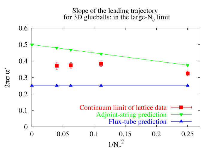
Figure 6.3: The slope $\alpha^{\prime}$ of the leading Regge trajectory in 2+1 $SU(N_{c})$ gauge theory, in units of $\frac{1}{2\pi\sigma}$, as a function of $\frac{1}{N_{c}^{2}}$

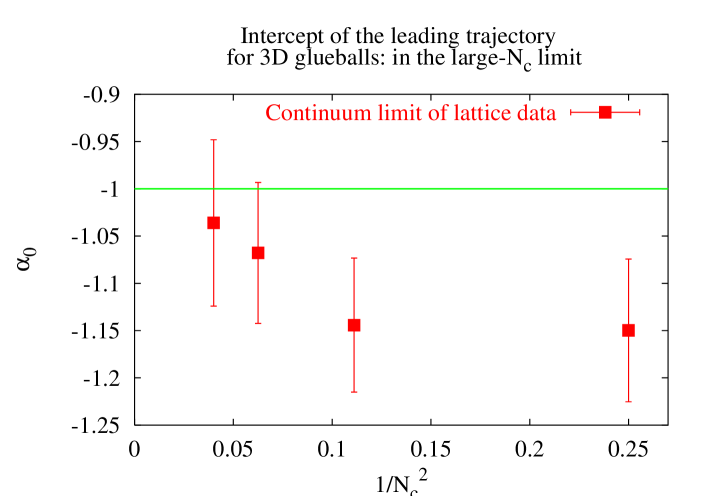
Figure 6.4: The intercept of the leading Regge trajectory, as a function of $\frac{1}{N_{c}^{2}}$ in 2+1 $SU(N_{c})$ gauge theory.

For all the $N_{c}$ considered, the lattice result for $\alpha^{\prime}_{m}$ is almost exactly midway between the two model predictions. We illustrate this fact in Fig. 6.3. We might speculate that even if both models are valid, thus producing two glueball trajectories with different slopes, at finite $N_{c}$ mixing will deform these trajectories from exact linearity and that such a deformation will be greatest at some lower $J$ where the states of the two trajectories are closest and also where we perform our calculations. We observe that the intercept of the leading Regge trajectory that we have obtained is close to -1, and becomes even closer at larger $N_{c}$, as we see on Fig. 6.4.

At finite $N_{c}$, Regge trajectories are not expected to rise linearly at arbitrarily large $t=m^{2}$. In particular we should expect that due to mixing between high spin glueballs and multi-glueball scattering states, for which $\alpha(t)\propto\sqrt{t}$, the local slope of the trajectory decreases as $J$ increases. We might be seeing the beginning of such an effect with the spin 6 state in $SU(2)$. This effect is, however, suppressed by $\frac{1}{N_{c}}$ in the large $N_{c}$ limit.

6.4.3 Implications for high-energy reactions

The contribution of the leading glueball trajectory to the total cross-section behaves as $\Delta\sigma\propto s^{\alpha_{0}-1}$, which means, given our calculated value $\alpha_{0}\simeq-1$ , that it is suppressed as $\sim s^{-2}$. Thus the high-energy scattering of glueballs is not dominated by Regge pole exchange in 2+1 dimensions; at least if we believe that cross-sections should be constant at high energies up to powers of $\log{s}$.

Going back to Section 6.1.1, we note that the other terms contributing to the scattering amplitude are the ‘fixed-pole’ amplitude $a_{0}$ and the ‘background integral’. Because there is a unitarity bound on each partial wave, the contribution of any partial wave amplitude to the total cross-section is bounded by $\sim s^{-1}$. Thus the $s$-wave amplitude will not dominate either at high energies. That, then, only leaves the background integral. If the partial wave amplitude $a(\lambda,t)$ were meromorphic in the region $0<{\rm Re}~{}\lambda<\frac{1}{2}$, we would simply get additional Regge pole contributions, which should show up as physical states by analytic continuation. Therefore there must be a more complicated singularity structure in that region. For instance it is well known that $\lambda=0$ is a logarithmic branch point of the partial wave amplitude $a(\lambda,t)$ at low energies (see [129] and Appendix C). Also, Li and Tan [130] remark that the dipole-dipole forward scattering amplitude can be written as a contour integral in the complex $\lambda$ plane around $\lambda=0$:

$$A(d,d^{\prime},s)=\frac{2\pi g^{2}d~{}d^{\prime}}{N_{c}}\frac{1}{\log{s}}=-\frac{2\pi g^{2}d~{}d^{\prime}}{N_{c}}\int\frac{d\lambda}{2\pi i}s^{\lambda}\log{\lambda}$$ (6.14)

where $d,~{}d^{\prime}$ are the sizes of the scattering dipoles; again, the logarithmic branch point seems to dominate the scattering process. This intriguing similarity suggests a universal contribution from the point $\lambda=0$.

6.5 Conclusion

We computed part of the higher-spin mass spectrum of $SU(2)$ gluodynamics in 2+1 dimensions. We have also revisited the data published in [66] and reassigned the spin quantum number.

Such calculations can tell us what the leading glueball Regge trajectory looks like and, in particular, whether it resembles the pomeron. Apart from the predictions of string models of glueballs, our motivation for a study in D=2+1 is an intuition that in high-energy scattering the colliding glueballs should behave like ‘black segments’ (analogous to the ‘black disks’ of D=3+1) so that the cross-section is approximately constant at high $s$. Of course in D=2+1 we have no experimental support for such an intuition and we therefore investigated how various field theoretic approaches to high-energy scattering can be translated from D=3+1 to D=2+1. The generic change is that infrared divergences become much more severe so that one can no longer predict a power-like dependence of the cross-section in $s$ directly from the BFKL equation [131]. However there exist alternative calculational schemes [130] which lead to constant cross-sections, up to logarithms.

The framework for Regge poles is Regge theory and we saw that there are qualitative changes when we go from 3 to 2 spatial dimensions. In particular the $\lambda=0$ partial wave is not included in the Sommerfeld-Watson transform and the Froissart bound is $\sigma_{\rm tot}\leq{\rm const.}\log s$. We speculate that the singularity structure at $\lambda=0$, which is not associated with particles of the theory, is promoted to a dominant contribution to the high-energy cross-section.

With this theoretical background in mind, we presented the results of our lattice calculation of the higher spin glueball spectrum. Extrapolating our masses to the continuum limit shows that the leading Regge trajectory in the (mass)² versus spin plane is in fact linear (to a good approximation) and contains only even-spin states. Moreover it has a small slope that lies roughly midway between the large-$J$ predictions of the flux tube and adjoint string models. The intercept at $t=m^{2}=0$ is $\alpha_{0}\simeq-1$. We identified a parallel daughter trajectory, lying about one unit of $J$ lower, containing all spins but spin 1. After reassigning the spin quantum number in data [66], we were also able to determine the two leading Regge trajectories for other $SU(N_{c})$ groups. We found that the result depends very little on $N_{c}$ – except that the subleading trajectory now contains approximate $C=\pm$ doublets. A very natural interpretation is that we are seeing a combined spectrum of a spinning open adjoint string and a vibrating closed fundamental string, the leading trajectory being associated with the former. Presumably states produced by either dynamics undergo a certain amount of mixing with those generated by the other degrees of freedom. The presence of the isolated $1^{\pm-}$ state is a hint at more complicated topologies of the string. Finally, we note that our results are relevant to the theoretically interesting $SU(\infty)$ limit.

The very low intercept of the leading glueball trajectory ($\alpha_{0}\simeq-1$) indicates that the moving Regge pole corresponding to these glueball states gives a negligible contribution to high-energy scattering in 2+1 dimensions. We concluded that there must be a more complicated singularity structure of the partial wave amplitude in the complex angular momentum plane $\lambda$. Evidence for a possibly universal branch point at $\lambda=0$ comes mainly from low-energy potential scattering (where the result is independent of the potential [129]) and is suggested by the $\frac{1}{\log{s}}$ scattering amplitude found by Li and Tan in $QCD_{2}$ high-energy scattering. These statements are quite different to what one expects in 3+1 dimensions.

IR	spin	$\beta=6$	$\beta=7.2$	$\beta=7.2$	$\beta=9$	$\beta=12$	$\beta=18$
		$L=16$	$L=20$	$L=40$	$L=24$	$L=32$	$L=50$
$\sqrt{\sigma}$		$0.2538(10)^{*}$	0.2044(5)	0.2072(46)	$0.1616(6)^{*}$	$0.1179(5)^{*}$	0.0853(14)
$A_{1}$	$0^{+}$	1.198(25)	0.981(14)	0.951(14)	0.7652(78)	0.570(11)	0.3970(78)
	$0^{+}$	1.665(43)	1.396(21)	1.394(18)	1.108(23)	0.847(18)	0.584(32)
	$0^{+}$	2.198(76)	1.859(25)	1.778(34)	1.426(37)	0.980(28)	0.717(76)
	$0^{+}$	2.27(10)	2.084(41)	2.067(54)	1.522(36)	1.226(17)	0.845(37)
	$4$	2.44(27)	2.07(33)	2.146(64)	1.570(39)	1.195(47)	0.798(32)
	$4$		2.53(13)	2.50(14)	1.700(52)	1.419(90)	0.963(45)
$A_{3}$	$2$	1.957(48)	1.584(18)	1.567(18)	1.232(38)	0.933(11)	0.634(18)
	$2$	2.08(18)	1.870(37)	1.891(39)	1.421(44)	/	0.667(20)
	$2$	2.34(25)	2.219(90)	2.242(77)	1.660(54)	1.152(42)	0.862(14)
	$2$	2.65(29)	2.451(71)	2.47(12)	1.746(56)	1.459(29)	1.019(92)
	$6$	2.93(21)	2.51(19)	2.64(15)	1.878(86)	1.438(28)	0.906(69)

IR	spin	$\beta=6$	$\beta=9$	$\beta=12$
$A_{2}$	4	2.423(34)	1.5766(96)	1.180(17)
	4	2.638(85)	1.772(44)	1.384(50)
$A_{4}$	2	1.908(48)	1.2372(73)	0.9191(33)
	2	2.04(13)	1.4619(73)	1.0920(51)
	2	2.310(36)	1.685(22)	1.2568(73)
	2	2.521(62)	1.777(39)	1.321(10)
	6	2.780(65)	1.932(84)	1.456(16)
$E$	3	2.520(60)	1.6732(97)	1.2547(54)

Table 6.2: The lightest states in the 2+1D $SU(2)$ gauge theory. The string tension values with an asterisk are taken from [66]. The data for the $A_{1}$ and $A_{3}$ representations was published in [4], the data for the $A_{2}$, $A_{4}$ and $E$ representations is more recent and unpublished.

IR	spin	$\beta=7.2$	$\beta=9$	$\beta=12$	$\beta=18$
$A_{1}$	$0^{+}$	1	1	1	1
	$0^{+}$	1	1	1	1
	$0^{+}$	1	1	1	/
	$0^{+}$	0.59(12)	0.68(62)	0.97(13)	1
	$4$	0.94(9)	0.98(4)	0.38(2)	0.95(2)
	$4$	/	0.67(16)	0.59(4)	0.98(3)
$A_{2}$	4			1
	4			0.98(2)
$A_{3}$	$2$	1	1	1
	$2$	1	1	1
	$2$	1	1	0.97(11)
	$2$	1	1	1
	$6$	/	0.87(8)	0.88(4)
$A_{4}$	2			1
	2			1
	2			/
	2			/
	6			0.19(2)
$E$	3			0.96(2)

Table 6.3: The Fourier coefficients of the spin $J$ states given in Table 6.2: $|c_{J}|^{2}$ at $\beta=~{}7.2,~{}9,~{}12$ and 18. When the coefficient is larger than 0.99, we round it off to 1.

Figure 6.1: The Chew-Frautschi plot of the continuum D=2+1 $SU(2)$ glueball spectrum.

Figure 6.2: The Chew-Frautschi plot of the relabelled continuum D=2+1 $SU(3)$ glueball spectrum obtained in [66].

Chapter 7 Glueball Regge trajectories in 3+1 dimensions

We investigate the spectrum of $SU(3)$ gauge theory in 3+1 dimensions and its relation to the pomeron. We shall also present a comparison with the spectrum of $SU(8)$ gauge theory, and argue that the latter is representative of the planar limit.

We first explain some lattice technicalities, and then show how our spin identification technique generalises to three space dimensions. We present our lattice data, along with a finite-volume study and a first attempt to understand the influence of double-torelon and scattering states on the extracted spectrum. An interpretation of the latter in terms of Regge trajectories is given. In particular, a pomeron-like trajectory is identified and its physical consequences at negative $t$ are discussed. The general conclusion is postponed to the next chapter.

7.1 Lattice technology

In this section we present the details of our operator construction procedure, as well as the strategy to label the glueball states with the correct spin quantum number.

7.1.1 Operator construction

It is well-known that the overlap of operators onto the lightest physical states of the theory can be greatly enhanced by methods such as smearing [105] and blocking [106]. We used several levels of the iterative procedure described below. Each step produces out of the links of the previous step a link that is ‘fatter’ and doubled in length. Thus a Wilson line with an index $(B)$ represents a line of length $2^{B}$ times the initial length. The operations at level $B=0,\dots N_{B}-1$ take the following form (initially, $U^{(0)}_{\mu}(x)=U_{\mu}(x)$):

1. If $B\neq 0$, double the length of the links produced at the previous level:

   $$U^{(B)}_{\mu}(x)~{}=~{}U^{(B-1)}_{\mu}(x)~{}~{}U^{(B-1)}_{\mu}(x+2^{B-1}a\hat{\mu})$$ (7.1)

2. Smear the links $U^{(B)}$ $n_{B}$ times: omitting the site and direction indices of the links,

   $$U^{(B)}_{S}=\left[~{}U^{(B)}_{S-1}~{}+~{}w^{(B)}_{S}~{}\Sigma^{(B)}_{S-1}~{}\right]_{\cal U},\qquad S=1,\dots,n_{B}$$ (7.2)

   where $\Sigma^{(B)}_{S-1}$ is the sum of staples made of the links $U^{(B)}_{S-1}$ and the lower index represents the smearing level. The operation $\cal U$ is a unitarisation procedure. We choose to maximise $\mathop{\rm Re}{\rm Tr\,}(UV^{\dagger})$ where $V\in GL_{N_{c}}(C)$ is the matrix to be reunitarised and $U\in SU(N_{c})$ is the result of this operation (see App. B). After the last smearing step, we call $U^{(B)}_{n_{B}}\equiv U^{(B)}$.

The number of smearing parameters $\{n_{B}\}^{N_{B}-1}_{B=0}$ and $\{w^{(B)}_{S}\}$ is large and it is hardly possible to undertake an optimisation program. Fortunately, it is well-known that the smoothness of the links is rather insensitive to the precise choice of parameters. We typically choose $0.35\leq w\leq 0.40$. We can now construct gauge-invariant operators out of $N_{B}$ sets of links, covering a range of physical sizes.

One simple observation is computationally useful. Any product of links along a closed path uses an even number of them. Therefore, if a large number of operators is to be measured, one can spare half of the $SU(N_{c})$ matrix multiplications if all paths of length 2 (we call them ‘wedges’ and ‘double-links’) in a time-slice are initially computed and stored. In 3 spatial dimensions there are 3 double-links going in the ‘up’ direction and (3 planes) $\times$ (4 wedges per plane) = 12 wedges to be computed and stored per site. This represents thus 15 matrix multiplications per site. In 2 spatial dimensions, there are 6 of them (2 double-links and 4 wedges per site). Any closed loop can then be computed by multiplying these Wilson lines end-to-end. Since the double-links need to be computed for the next level of the link-fattening procedure $B+1$, the actual computational overhead to obtain these building blocks is 12 (4) matrix multiplications in 3 (2) spatial dimensions. For instance, suppose the simplest operator without any intrinsic symmetry is being measured (sometimes called the ‘hand’ in $D_{s}=3$, while in $D_{s}=2$ it is the ‘knight’s-move’). These operators come in a large number of copies (48 and 8 respectively), each of which requires 6 (resp. 8) $SU(N_{c})$ multiplications. If the wedges and double-links have been stored, each of the copies only requires half as many multiplications. Thus the initial overhead is seen to be very small indeed, and the gain is practically a factor 2 in speed. Note that we did not have to make any restricting assumptions about the operators that are going to be measured. Naturally, further increase in speed is possible if it is decided at compiling time which operators are going to be measured, or if the program is ‘intelligent’ enough to find by itself, before the very first measurement of the simulation, the optimal order in which to do all the necessary matrix multiplications for the measurements.

The memory requirements of this operator-construction program are relatively large but not prohibitive: only one level $B$ of the fattened links needs to be stored at a time, if measurements and link-fattening steps are alternated. The use of the double-links and wedges requires 15 (6) of them to be stored per site in $D_{s}=3~{}(2)$, rather than 3 (2) links.

Our spin-identification method requires a set of ‘probe’ operators (Chapter 4). Therefore we want to construct a set of spatial Wilson loops roughly of the size of glueballs $d$ which are obtained from each other through rotations by an angle $\varphi_{n}=\frac{2\pi}{n}$. Because the lattice breaks the rotation group $SO(3)$ down to the cubic group $O_{h}$, this can only be done (and is only meaningful) up to order $\left(a/d\right)^{2}$ corrections.

In ref. [121] and [1], an elegant definition of the propagation of flux was formulated (see Chapter 4). In brief, it involves computing the propagator of a fundamental scalar field, of bare mass $m_{0}$ and confined to a time-slice, on the gauge field background. The propagator taken between two points is a sum of Wilson lines along all possible paths, whose weighting is determined by their length $\ell$ and is given by $\alpha^{\ell}$ where

$$\alpha=\frac{1}{(am_{0})^{2}+2d}$$ (7.3)

($d$ is the number of space dimensions). In [1] it was shown in the free case (all links are unit matrices) that in the regime $a\ll d\ll m_{0}^{-1}$, the propagator is dominated by paths of length $\ell\gg d$ and that the rotation symmetry is restored up to $\left(a/d\right)^{2}$. This means that at least in principle, for any desired accuracy and fixed physical length scale, there exists a small enough lattice spacing such that the propagation of a scalar particle on that physical length scale looks spherically symmetric. If we use this propagator to construct gauge-invariant operators, the same statement will apply to them.

We did not pursue that particular method because of its computational cost. Instead we use smeared links to construct our operators, that is, the level $B=0$ set of operators described above. In Chapter 4 it was shown in 2+1D simulations that such an approach worked just as well at the lattice spacings typically used.

7.1.2 Spin identification on a cubic lattice

The decomposition of $SO(3)$ irreducible representations in cubic group representations leads to a set of degeneracies in the continuum limit. These degenerate lattice states merge into a single continuum state of definite spin. They can thus be considered as different polarisations of the same state. The set of degenerate states depends on the spin. The expected degeneracies (see Appendix A) lead to some simple signature rules: for instance, the spin 4 is the smallest that yields a degeneracy between an $A_{1}$ and an $E$ state, while the spin 6 is the smallest that yields a degeneracy between an $A_{2}$ and an $E$ state. Naturally higher spins can lead to the same degeneracies: just relying on these rules, one could mistake a spin 8 for a spin 4, or a spin 7 for a spin 6. They gradually become less useful: for instance, a spin 12 state simply appears 12 times in the $A_{1}$ representation!

But in practice, there are more severe limitations to this method. ‘Accidental’ degeneracies can appear for dynamical reasons. If we were to measure the hydrogen atom spectrum on the lattice, the method would be completely inapplicable, due to the independence of the spectrum on the angular momentum quantum number; a specificity of the Coulomb potential. While we do not expect such an extreme situation to occur in the case of glueballs, the density of states increases very rapidly with energy, and by the time the splitting between states becomes comparable to statistical error bars, the method becomes insufficient.

We therefore need additional information, and we rely on a direct measurement [1] of the transformation properties of the lattice states under ‘approximate rotations’, as defined in Section 7.1.1, by angles smaller than $\pi/2$. Before we describe the procedure in detail, we work out what wavefunctions we expect to find in the continuum limit. Let us consider for instance a spin 2 state. In the continuum, its five polarisations, labelled by the projection $m$ of the spin on a chosen $z$ axis, are described by the spherical harmonics $Y_{2}^{m}$, $-2\leq m\leq 2$. On the lattice, these polarisations get rearranged into two lattice irreducible representations, $E$ (2-dimensional) and $T_{2}$ (3-dimensional). Since we are always measuring states belonging to definite lattice representations, the question is then, which linear combinations of the $\{Y_{2}^{m}\}$ are bases of $E$ and $T_{2}$. It is easy to check that $\{Y_{2}^{2}+Y_{2}^{-2},Y_{2}^{0}\}$ form an orthogonal basis of $E$, while $\{Y_{2}^{2}-Y_{2}^{-2},Y_{2}^{1},Y_{2}^{-1}\}$ span $T_{2}$.

A more complicated case arises for the spin 4 state. We know from group theoretical arguments that a unique linear combination of $\{Y_{4}^{m}\}$ belongs to the trivial lattice representation $A_{1}$. Given that an $A_{1}$ state is invariant under $\frac{\pi}{2}$-rotations around the $z$ axis, only $Y_{4}^{0}$ and $Y_{4}^{\pm 4}$ can contribute. Symmetry about the $xz$ and $yz$ planes imposes the couple $Y_{4}^{\pm 4}$ to come in the combination $Y_{4}^{4}+Y_{4}^{-4}$. The relative weight of the latter and $Y_{4}^{0}$ is finally determined by requiring that the combination be invariant under a $\frac{\pi}{2}$ rotation around the $y$-axis. This linear combination can be obtained by diagonalising the $D$-matrix $D(0,\frac{\pi}{2},0)$ which describes the rotation parametrised by Euler angles $(\alpha,\beta,\gamma)$ in the basis of spherical harmonics: the correct linear combination

$$\lambda Y_{0}^{0}+\frac{\mu}{\sqrt{2}}(Y_{4}^{4}+Y_{4}^{-4})$$

is the eigenvector with eigenvalue $+1$. $\lambda$ and $\mu$ are thus known numerical coefficients. A complete decomposition of the $J\leq 6$ representations obtained in this way is given in Table (7.7). Let us repeat what these linear combinations represent in the case of the polarisation of the spin 4 state lying in the $A_{1}$ representation: it is the wave function of a true, continuum spin-4 particle prepared in a state that is invariant under all the symmetry operations of the cubic group.

The linear combinations thus merely reflect the fact that we measure the states in specific polarisations, which we choose to correspond to lattice irreducible representations. Naturally, the lattice states will in general have wave functions which are a mixture of these specific polarisations. A discretised wave function will be defined below, with a discretisation angle $\Delta\varphi={\cal O}(a/d)$, where $d$ is the size of the state. As $a\to 0$, we expect such a wave function to approach one of the allowed linear combinations appearing in Table (7.7) that corresponds to a continuum state. There is however a circumstance where even this expectation can be in default: that is the mixing of ‘accidentally’ near-degenerate states, when $\Delta E/\sqrt{\sigma}={\cal O}(\sigma a^{2})$. Because the glueball density of states increases strongly beyond the first $\sim 10$ states, at any finite lattice spacing the near-degeneracies eventually overwhelm the strict separations between states belonging to different continuum multiplets and the lattice state wave functions bear no resemblance with their continuum counterparts. Such mixings would also affect the energy levels themselves. Thus a small lattice spacing is mandatory to compute the excited spectrum.

We now consider the actual wave function measurement. We shall make use of the notation

$$|J~{}\{m\}~{}\rangle = \frac{1}{\sqrt{2}}\left(~{}|J,~{}m\rangle~{}+~{}|J,~{}-m\rangle~{}\right)$$

$$|J~{}[m]~{}\rangle = \frac{1}{\sqrt{2}}\left(~{}|J,~{}m\rangle~{}-~{}|J,~{}-m\rangle~{}\right).$$ (7.4)

The phases are chosen such that $\langle\theta~{}\phi|J,~{}m\rangle=Y_{J}^{m}(\theta,\phi)$, where $\theta,\phi$ are the spherical coordinates with respect to the lattice axes. Let $\{\Psi^{(n)}\}_{n=0}^{N}$ be a set of operators, such that $\Psi^{(n)}=U^{\dagger}(\phi_{n})\Psi^{(0)}U(\phi_{n})$, where $\phi_{n}\simeq\frac{2\pi}{n}$ and $U$ is a representation of the $SO(2)$ rotation group approximately realised around the (0 0 1) direction of the lattice on length scales $d\gg a$. Suppose furthermore that $\Psi\equiv\Psi^{(0)}$ acting on the vacuum creates an eigenstate of the transfer matrix (we slightly abuse the notation by using the same symbol to denote the state and the operator). The angular function

$$g(\phi_{n})~{}\equiv~{}\langle\Psi^{(n)}|\Psi^{(0)}\rangle$$ (7.5)

characterises the state created by $\Psi$. Let us consider as an example $\Psi\in A_{1}$. Then

$$|\Psi\rangle=|\psi_{0}\rangle~{}|0,~{}0\rangle~{}+~{}|\psi_{4}\rangle~{}\left(~{}\lambda~{}|4,~{}0\rangle~{}+~{}\mu~{}|4~{}\{4\}\rangle~{}\right)~{}+~{}\dots$$ (7.6)

where $\lambda,\mu$ are known ($\lambda^{2}+\mu^{2}=1$) and the dots refer to contributions of higher spin states. We have

$$g(\phi)=||\psi_{0}||^{2}~{}+~{}\lambda^{2}||\psi_{4}||^{2}~{}+~{}\mu^{2}||\psi_{4}||^{2}\cos 4\phi$$ (7.7)

Therefore the measurement of the Fourier coefficients of $g(\phi)$ allows us to determine $||\psi_{0}||^{2}$ and $||\psi_{4}||^{2}$. These numbers, whose sum we normalise to 1, represent the ‘probability’ for the lattice state to be a spin 0 or spin 4 state. Indeed, if we consider an effective continuum theory that is equivalent to the lattice theory [134], then the lowest-dimensional (irrelevant) operator that breaks rotational symmetry is of dimension six (we are using the Wilson action). We know that such an operator has the effect of introducing ${\cal O}(a^{2})$ corrections in the mass ratios of the theory. Suppose that we start with a basis of states lying in irreducible representations of the $SO(3)$ rotation group. First-order perturbation theory then tells us that the energy eigenstates acquire new components of ${\cal O}(a)$ in presence of the irrelevant operator; and therefore, in the example considered above, either $||\psi_{0}||^{2}$ or $||\psi_{4}||^{2}$ is ${\cal O}(a^{2})$.

In general, to obtain the wave functional $\Psi$ of a glueball, the variational method [108] has to be applied on a large basis of operators. This method yields a matrix (ideally) giving the components of energy eigenstates in the original basis of operators. The same linear combinations of the rotated copies $|\Psi^{(n)}\rangle$ can be taken to extract the angular wave function as described above. Although the method is general and has been applied in practice (see [1] and Chapter 4), the condition that we must be able to rotate the operators by small angles is quite a restrictive one to impose on the trial operators. Therefore a generalisation was considered in [4] (see Chapter 6). We give ourselves a set of ‘probe’ operators $\{P^{(n)}\}_{n=0}^{N}$, $\langle P^{(n)}~{}P^{(n)}\rangle=1$. The method now consists in measuring

$$g_{P}(\phi_{n})\equiv\langle P^{(-n)}\Psi\rangle=\langle P_{0}\Psi^{(n)}\rangle\qquad\forall n,$$ (7.8)

The equality relies on the invariance of the vacuum under the rotation. An example of probe operators used in the $PC=++$ sector is illustrated on Fig. (7.1). In that sector the identification requires the most care, given the relatively large density of states.

Figure 7.1: A typical set of Wilson-loop probes $P_{n}$ used for the wave-function measurement in the $PC=++$ representations.

In the case of $\Psi\in A_{1}$, we could use for $P$ the sum of two orthogonal rectangular Wilson loops illustrated on Fig. (7.1). If $P$ is the combination lying in planes (1 0 0) and (0 1 0), then it belongs to a reducible representation $A_{1}\oplus E$. Therefore

$$|P\rangle=|p_{0}\rangle~{}|0,0\rangle~{}+~{}|p_{2}\rangle~{}|2,0\rangle~{}+~{}|p_{40}\rangle~{}|4,0\rangle~{}+~{}|p_{44}\rangle~{}|4\{4\}\rangle~{}+~{}\dots$$ (7.9)

and

$$g_{P}(\phi)=\langle p_{0}|\psi_{0}\rangle~{}+~{}\lambda\langle p_{40}|\psi_{4}\rangle~{}+~{}\mu\langle p_{44}|\psi_{4}\rangle~{}\cos 4\phi.$$ (7.10)

The Fourier coefficient of $\cos 4\phi$ thus informs us about

$$c_{4}=\mu\langle p_{44}|\psi_{4}\rangle.$$ (7.11)

By the Schwarz inequality,

$$||\psi_{4}||^{2}\geq\frac{|\langle p_{44}|\psi_{4}\rangle|^{2}}{||p_{44}||^{2}}=\frac{|c_{4}|^{2}}{\mu^{2}||p_{44}||^{2}}.$$ (7.12)

$||p_{44}||^{2}$ may be determined by ‘probing the probe’ itself, as described above, or the probe can be made to have a spin 4 wave function by construction. We can thus determine lower bounds for the amount of spin 4 admixture in the $A_{1}$ states. Now the Fourier coefficients can no longer be extrapolated to the continuum, but in practice it turns out that this is not absolutely necessary on the relatively small lattice spacings that we are using. Although we have through this generalisation decoupled the task of constructing good glueball operators from the spin assignment problem, it is crucial that the probes should have a substantial overlap onto the glueball operators $\Psi$. If that is not the case, the lower bound set by the Schwarz inequality will not allow us to discriminate between spin 4 and spin 0. Given that close to the continuum, $||\psi_{4}||^{2}$ is of order ${\cal O}(a^{2})$ for a quasi-spin 0 state, the overlap $\langle P|\Psi\rangle$ must be significantly larger than ${\cal O}(a)$ for the bound to be useful. Clearly, as smaller lattice spacings are used, this condition on the probe weakens, but it is still non-trivial at the lattice spacings at which we can afford to do simulations.

7.2 The quenched QCD spectrum from the lattice

We performed six Monte-Carlo runs at four different lattice spacings (see Table 7.2). The two extra runs were used to estimate finite-volume effects, as well as the importance of mixing of the single-glueball states with 2-torelon and 2-glueball states. We were using a 2-level algorithm [2] as described in Chapter 5. The number of measurements performed at fixed time-slices was 40. The choice resulted as a compromise between improving the accuracy of the heavy-glueball correlators and maintaining a reasonable efficiency for the lighter ones. Ten compound sweeps separated two sets of ‘fixed’ time-slices. While the boundary time-slices are kept fixed, we perform two compound sweeps between the measurements, since the number of measured operators was large.

In the following we describe the spin identification procedure in practice, the study of finite-volume effects and the evaluation of mixing between our operators and 2-glueball and 2-torelon states.

7.2.1 Spin identification in action

Let us consider for instance the data at $\beta=6.4$ ($a\simeq 0.05$fm) and start with the $A_{1}^{++}$ representation. We will first try and see how far we can go with the degeneracy arguments. The smallest spins appearing in this representation are 0, 4, 6 and 8. The first two states clearly have no degenerate partners in the other representations, therefore they must be spin-0 like. The first two states in the $E$ and $T_{2}$ obviously match, and match no other states; therefore they must be spin-2 partners.

In the region $0.85<am<1.0$, there are altogether eight lattice states (see Table 7.1). Since one of them is $A_{2}$, a state with spin 3, 6 or higher must be involved; and we ignore the $A_{2}^{*}$ for the moment. One possibility is that this collection of states corresponds to a spin 6, a spin 0 and a spin 1 state. Another possibility is that we have a spin 3, a spin 4 and a spin 0 state. A third possibility is a spin 3, a spin 2, a spin 1 and two spin 0. We got stuck!

Now we will make use of the information coming from the wave function measurements, Table 7.8. The state in the $A_{2}$ representation appears to have no $\cos{6x}$ component in its wave function, within the systematic uncertainty of the wave function measurement. Thus the first-mentioned possibility is practically excluded. We can pair the ($A_{2}$, $T_{1}$, $T_{2}$) together to form the seven polarisations of a spin-3 state. The question is now whether a spin 4 state is present or not. The wave function measurement provides no evidence for the $A_{1}^{**}$ being a spin 4. But the $A_{1}^{***}$, the $E^{**}$ and the $T_{1}^{*}$ all have spin-4 components that are at least five times larger than the expected scale of the rotational symmetry breaking. Therefore with all likelihood these lattice states correspond to different polarisations of a spin 4 state. The $T_{2}^{***}$ completes the nine polarisations. The absence of additional states in the $T_{1}$ and $T_{2}$ representations that are near-degenerate with the $A_{1}^{**}$ state confirms the scalar-like nature of the latter. It should be noted that there is an extra state in the $E$ representation, but that state was seen at all lattice spacings without a partner state in the $T_{2}$ representation and is found to have a strong volume dependence. The only way this can happen systematically is if it corresponds to a two-torelon state. It is an infrared breaking of rotational invariance, which we shall come back to in the next section.

The wave function analysis of $A_{2}^{*}$ exhibits no $\cos 6\phi$ component, and therefore it almost certainly corresponds to a spin 3 state. The next state, $A_{2}^{**}$ has a large component of this type and hence it must be one of $J=6,7,9,\dots$ A near-degenerate state is seen in the $E$ representation, although its overlap onto the probe is too small to allow us to determine the angular dependence of its wave function with confidence. Also, a degenerate state in the $A_{1}$ representation is seen, and it has a strong $\cos 4\phi$ component; if the degeneracy is not accidental, this rules out the possibility $J=7$. While we cannot rule out accidental degeneracies, the ($A_{1}$, $A_{2}$, $E$) triplet thus most probably corresponds to a spin-6 state.

The combination of the degeneracy arguments and the wave function measurements thus allows us to disentangle the states. In the other $PC$ sectors, the density of states below 4GeV is not as high and the degeneracies are usually sufficient to determine the spin-multiplets. An interesting case arises in the $PC=-+$ sector. The first two $T_{1}$ states are almost degenerate at all lattice spacings; and the $A_{2}$ state is very high-lying, and so is the $A_{1}^{**}$ above the two low-lying pseudo-scalars. This excludes the possibility that one of the $T_{1}$ states can belong to a spin 3 or spin 4 multiplet. Furthermore, we see that the $T_{2}^{**}$ state is quasi-degenerate. So unless we are seeing an accidental degeneracy between three (!) states (two spin 1 and a spin 2), the $T_{1}$, $T_{1}^{*}$, $E^{**}$ and $T_{2}^{**}$ must correspond to a spin 5. Furthermore, an unpublished set of data, where the glueball operators allowed us to measure the spin components directly (see Eqn. 7.7), tells us that at least one of the $T_{1}$ states has large variations in its $\phi$ dependence, which excludes the $J=1$ interpretation.

In the $PC=+-$ sector, a striking degeneracy at all lattice spacings of the $E$, $T_{1}^{***}$ and $T_{2}^{***}$ states suggests a spin 4 or spin 5 multiplet. We are unable to say whether another $T_{1}$ state is near-lying (which would complete the spin 5 multiplet), or whether instead the $A_{1}$ state is degenerate with these lattice states. If we combine our data with that given in [111], where the $A_{1}$ state was found to be definitely heavier than the $E$ state, it would appear that we are actually seeing a spin 5 multiplet (a gap above the $T_{2}^{***}$ excludes the possibility of a spin 3 – spin 2 degeneracy). In this case we feel however that the labelling requires confirmation, in particular the missing $T_{1}$ state should be seen to complete the multiplet.

7.2.2 Bi-torelon states and other finite-volume effects

Tables (7.4) and (7.5) show the relative variation of the energy levels as the volume is varied between 1.4 and 2.0fm (runs IV, V, VI at $\beta=6.2$). Almost all levels undergo variations that are consistent with zero, within 1-1.5$\sigma$. Exceptions are highlighted in the table: they concern the $A_{1}^{++*}$ and the $E^{++}$ states, as well as a state appearing in the $E^{++}$ representation which has no analog in the $T_{2}^{++}$, and which we labelled as ‘2T’. It is the only state for which we see a definite trend of increasing mass with the volume. We therefore interpret it as a finite-volume effect. Apart from this special case, the largest effect is observed for the $0^{++*}$ state on the 1.4fm lattice (2.7 standard deviations). A similar volume dependence for this state was also observed in [111].

Naturally these variations (apart from the 2T case) could simply be statistical fluctuations. We noticed empirically that the variational calculation can in some cases amplify the statistical fluctuations, since it finds by definition the linear combination of operators that minimises the local effective mass, which has a non-zero variance; the systematic error due to this enhancement is typically not included in quoted statistical errors. If it is a physical effect, it is somewhat peculiar that these states are lighter both on the smaller and the larger volumes. Also, in the case of the lightest $E^{++}$ state, the partner state in the $T_{2}^{++}$ representation shows no sign of volume dependence. There is a well-known finite-volume effect that can explain a mass difference between two states in the $E^{++}$ and $T_{2}^{++}$ representations corresponding to the same continuum state, as well as the appearance of an extra state in $E^{++}$.

The torelon, a state created by a Polyakov loop in the fundamental representation, transforms non-trivially under the centre symmetry ${\bf Z}_{N_{c}}$ of the gauge group $SU(N_{c})$. The product of two such operators winding in opposite direction, however, has trivial transformation properties under the global ${\bf Z}_{N_{c}}$ symmetry and can therefore create states that mix with glueballs. In physical terms, fusion of flux-tubes can occur, after which the newly formed loop is contractible. The general consequence is that extra states are seen in the finite-volume ‘glueball’ spectrum with respect to the infinite volume limit, where the bi-torelon states become infinitely massive and decouple. The two cubic representations that can be affected by the extra states are the $A_{1}^{++}$ and $E^{++}$.

In the two simulations (run IV and VI, Table 7.2) designed to check for finite-volume effects, we explicitly included the measurement of products of (fuzzy) Polyakov loops. We use operators which have zero total momentum, and zero relative momentum. A plot of their local effective masses as function of Euclidean time is shown in Fig. (7.2). We firstly note that although there is no symmetry preventing the decay of the observed plateaux toward the lightest glueball energy level, this does not happen in the range where we are able to measure the correlator accurately. We conclude that the bitorelon has very little overlap onto the lightest glueball. Secondly, the mass plateaux are very much lower than the value for two non-interacting flux-tubes, and the lowering increases with the length of the torelons. This behaviour is qualitatively very different from the case of a two-glueball scattering state (see below).

To understand their effect on the $A_{1}^{++}$ and $E^{++}$ spectrum, we give the energy levels resulting from the variational calculation with, and without the bi-torelon operator included in the starting basis (Table 7.6). In the $A_{1}$ case, we use the superposition of bi-torelon states winding around all three cycles of the torus, while for the $E$ we use only the one winding in the $z$-direction (whilst the other $E$ operators are of the type $Y_{2}^{0}$). The overlap $|\langle{\cal O}_{G}{\cal O}_{2T}\rangle|$ between the bi-torelon operator and the ordinary operators prior to diagonalisation is less than 0.1 in the $E$ case and $0.2-0.3$ in the $A_{1}$ case; they only decrease slightly as the spatial extent of the lattice is increase from 1.4 to 2fm. The generic effect we observe is that a new, relatively light state appears - which we did not ‘see’ on the original volume.

The $A_{1}$ and $E$ spectra without the inclusion of the bi-torelon operator are very similar on all three volumes, with one exception: on the small volume (run IV), there is an extra light state in the $A_{1}$. It may correspond to the lightest scattering state or a bi-torelon state. In both the 1.4 and 2.0fm boxes, the inclusion has the general effect of producing a relatively ‘noisy’ extra state. We note again that the new state is significantly lighter than the naive sum of two torelon masses (Table 7.2), especially in the $E$ case. We infer that the force between two torelons is strongly attractive. Interestingly, the $A_{1}^{++*}$ in the 2.0fm box, which appeared to be lighter by $~{}2\sigma$, is now back to the value obtained in the 1.7fm box (Table 7.1), although it is now much noisier.

Figure 7.2: The local effective mass of bi-torelon operators, at $\beta=6.2$ (runs IV and VI). The $A_{1}$ representation is obtained by superposition of the bi-torelon operators winding around each cycle of the hypertorus, while the ‘single’ corresponds to just one of them. The expectation for two non-interacting flux-tubes is indicated by the horizontal lines. A fit to the $A_{1}$ mass plateaux yields 0.787(39) and 1.02(6) for $L=20$ and 28 respectively.

In conclusion, the bitorelon states mix with the $A_{1},E^{++}$ glueball states, but the extra states introduced as a result of the mixing become heavier as the extent of the spatial lattice is increased. The anomalous behaviour of the $A_{1}^{++*}$ energy level as a function of the volume may be due to the proximity of a two-torelon energy level, which only appears explicitly in the variational spectrum if two-torelon operators are included in the basis. The case of the fundamental state in the $E^{++}$ representation is harder to understand: it comes out lighter on either smaller or larger volume than the standard volume ($L\simeq 1.7$fm), whether or not the bi-torelon operator is included. We are therefore inclined to consider this particular variation as a statistical fluctuation.

7.2.3 Scattering states $\&$ decays

When we apply the variational method to extract the fundamental and several excited states in a given symmetry channel, we do not know a priori the nature of these states. We need additional information to label the state with continuum quantum numbers, as discussed above. Another procedure needs to be followed in order to conclude that the linear combination obtained corresponds to a single glueball state, and not to a scattering state of several glueballs. In [111], the issue was sidestepped by only considering states that are below the two-particle threshold, which was estimated using the free relativistic dispersion relation. This approach proved sufficient to obtain a large number of states in the low-lying spectrum.

It is well-established [109] that decay widths of infinite-volume states and energy levels of scattering states in a finite volume are intimately connected. As a first attempt to study the effects of the two-particle threshold, we include direct products of traced Wilson loops with zero relative momentum into our basis of operators. Let us suppose that each of these operators, having very high overlaps onto physical states, creates one particular glueball. First consider for simplicity the planar limit $N_{c}\rightarrow\infty$. Due to the factorisation property we expect that the direct product creates two non-interacting glueballs. In this free-particle limit, each of the Wilson loops can be assigned a definite momentum ${\bf p_{1,2}}$. If the two glueball states have equal mass, in the centre-of-mass frame we simply have ${\bf p_{1}}=-{\bf p_{2}}$. In what follows we only consider the simplest case: the product of two of the operators creating the lightest glueballs ($0^{++}$) with ${\bf p_{1}}={\bf p_{2}}=0$. Now at finite $N_{c}$, this is not an eigenstate of the Hamiltonian, and therefore it can a priori have a finite overlap with any of these eigenstates, provided it has quantum numbers $0^{++}$ and ${\bf p}=0$. If we normalise the eigenstates and the direct product operator ${\cal O}$ such that $\langle n|n\rangle=1$ and $\langle{\cal O}~{}{\cal O}^{\dagger}\rangle=1$, unitarity implies that the sum of all the overlaps must add in quadrature to 1. In Table (7.9), we show the overlaps $|\langle\Omega|{\cal O}|n\rangle|$ of such ‘2-lightest-glueball’ (2LG) operators onto the orthogonal operators whose mass plateaux yielded the spectrum in Table (7.1). The overlaps are under the $10\%$ level. The dependence on which of the two 2LG operators is being used gives us a measure of the systematic uncertainty on the values obtained. The fact that the overlaps are tiny tells us that the 2LG operators are creating states that are practically orthogonal to our original basis of single-glueball operators.

The same conclusion can be reached in a different way. If we include either of the 2LG operators in the variational calculation, we obtain an extra state with mass $am=1.047(33)\simeq 2am_{0^{++}}$, which gets most of its contribution from the 2LG operator. The other 0++ states are unaffected within statistical errors by the inclusion of the extra operator. This provides some evidence that the states we extract above 2-particle threshold (starting with the $0^{++**}$) are narrow glueball resonances, since our variational basis does not resolve the 2-particle threshold. Two of the lightest glueballs seem to fit easily in the 1.75fm box without interacting (much): the extra mass plateau we obtain by including 2LG operators is within statistical errors twice the mass of the lightest glueball.

In general, the mass of resonances must be inferred from energy shifts [109] in the two-particle spectrum as the size of the periodic box is varied. However, for very narrow resonances, the energy levels become volume-independent (up to exponentially small corrections). And the correlator of the interpolating operator creating the quasi-state from the vacuum will have a long mass plateau before ‘decaying’ toward the energy of the scattering state. If operators are used that overlap very little onto the decay product of a quasi-stable state, it can be very hard to see the transition occur; a typical example is the measurement of the adjoint string tension with Wilson loops [133]. Given our observation that in general single-trace and double-trace operators have little overlap, we expect our unstable-glueball operators to produce long ‘meta-stable’ mass plateaux before the effects of the decay show up – and this is largely what is seen in the data. Finally, the observation of the multiplets corresponding to the $SO(3)$ representations are again useful cross-checks in this context, since the representations of $O_{h}$ contain different sets of scattering states.

It should also be remembered that the finiteness of the variational basis implies that the linear combinations of operators obtained cannot be strictly orthogonal in the infinite-dimensional space of operators. This means that we can never strictly obtain stable mass plateaux above the fundamental one – although in practice it is sufficient that they be long enough that a fit over several points may be done. It remains a small source of systematic error nonetheless. To illustrate these points we show a large number of mass plateaux in the $PC=++$ sector on Fig. (7.3) at our smallest lattice spacing ($\beta=6.4$). Recall that we usually do not store the very-short-distance correlator, so that the first local-effective-mass value occurs at 2.5 lattice spacings ($\sim$0.13fm). The representation where we could resolve the most states, and where the 2-particle threshold is lowest, is naturally the trivial one ($A_{1}$). According to Table (7.1), the threshold is around $aE=0.80$. Therefore only the fundamental $A_{1}^{(0)}$ and the first radial excitation $A_{1}^{(1)}$ are actually stable states. While the $A_{1}^{(2)}$ and $A_{1}^{(3)}$ (corresponding to a mixture of $0^{++**}$ and $4^{++}$) show reasonably long plateaux, $A_{1}^{(4)}$ is seen to decay into a lighter state quite ‘rapidly’ in Euclidean time, which could be the lightest scattering state of two of the lightest glueballs with zero relative momentum. In the $A_{2}$ representation (bottom plot), the first two states (corresponding to $3^{++}$) are stable, and the third mass-plateau (corresponding to $6^{++}$), which is above threshold, shows reasonable stability as well, although the error bars are larger.

Similar qualitative observations can be made about the mass plateaux in the $E$ and $T_{2}$. Although we know that they must be stable, because they are below threshold, the first excited state in each of these representations seems to be decaying into the lightest state. This is therefore most probably the above-mentioned effect of the finiteness of the variational basis, which implies that we cannot project out exactly the wave function of the fundamental state. Whilst the $E^{(2)}$ and $T_{2}^{(3)}$ states (corresponding to different polarisations of the spin 4 glueball) have very good plateaux, the effective-mass of the $T_{2}^{(4)}$ exhibits no plateau at all, and thus shows that the method has its limitations; in this particular case, the basis used in the variational calculation contained ten operators.

7.2.4 Continuum extrapolation and polarisation-averaged spectrum

Our continuum extrapolation is entirely conventional. Having obtained the spectrum at lattice spacings 0.05-0.10fm, we extrapolate the glueball spectrum in units of the string tension to the continuum, using a linear fit in $\sigma a^{2}$. This is the most natural scheme to set the scale in view of our forthcoming discussion of Regge trajectories. The resulting continuum spectrum is given in Tables (7.10) and (7.11). We are usually able to include all four points in the fit and have an acceptable value of $\chi^{2}$. In a few cases we drop the data at $\beta=6.0$, our coarsest lattice spacing. The extrapolations are illustrated on figs. (7.4–7.7).

The extrapolations of a few states produce bad $\chi^{2}$, for instance the lightest $0^{-+}$ state and the $3^{++}$ state in the $T_{1}$ representation. Upon inspection of Fig. (7.6), it seems very unlikely that this should be due to a violation of the scaling behaviour: the data points are ‘oscillating’ around the best fit line. We rather take it as an indication that the error bars are somewhat underestimated – they are purely statistical. Another general comment is that the data points at the finest lattice spacing ($\beta=6.4$) are often above the best-fit line, or have a significantly larger error bar. This is due to the fact that it is harder to achieve good overlaps onto the physical states at smaller lattice spacings; it is precisely this difficulty that prompted the development of techniques such as smearing [105] and blocking [106].

When a continuum state appears in several cubic representations, we note a remarkable agreement of the corresponding energy levels in the continuum limit. Given this fact, it is reasonable to average the energy levels to produce a final estimate of the energy level in units of the string tension. To do so, we weight the representations inversely proportionally to the square of their error bars. The final error bar assigned is conservatively taken to be the smallest error bar of the individual representations (rather than the expression $(\sum_{i}\Delta_{i}^{-2})^{-1/2}$ valid for a large number of data points). The result is given in the last column of Tables (7.10) and (7.11). To obtain the spectrum in physical units, we use $\sqrt{\sigma}=(440\pm 20)$MeV, which leads to the values given in Table (7.12).

Previous work

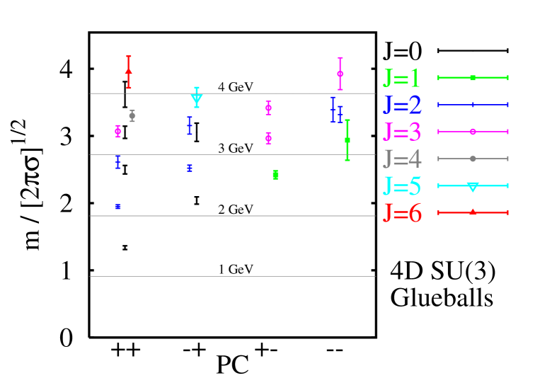
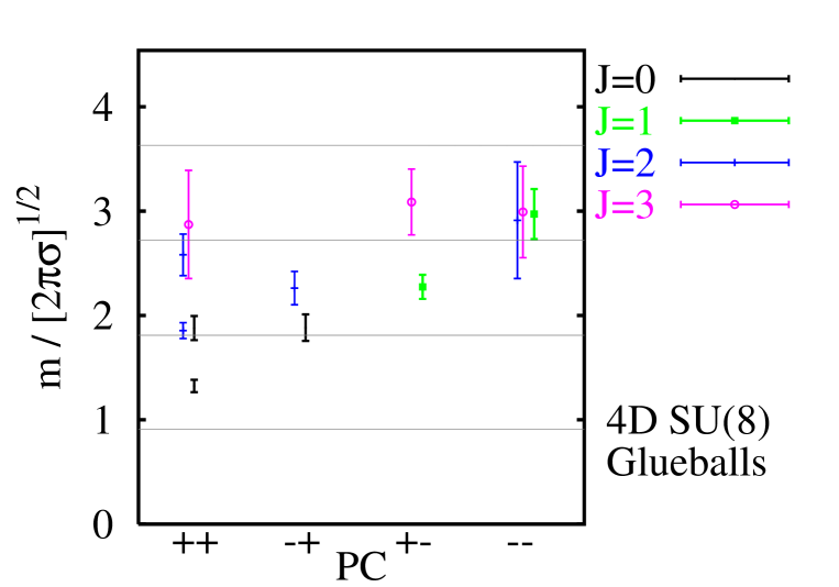
Figure 7.8: The continuum spectrum of glueballs in the 4D pure $SU(3)$ and $SU(8)$ gauge theories. The physical scale was set using $\sqrt{\sigma}=440$MeV.

Globally, our spectrum is in good agreement with that of Morningstar and Peardon [114] (see Fig. 7.8). There is a tendency for us to get the energy levels lower, in particular the mass gap is smaller in our data; also, our $1^{--}$ state is quite a bit lighter than in [114], although the accuracy of our continuum $PC=--$ energy levels suffered from the poor data at our smallest lattice spacing. Nevertheless, the $1^{--}$ level shows very little dependence on the lattice spacing, so that any of our data points would lie well below the value of [114].

In Ref. [135], Liu and Wu obtain the value 3.650(60)(180)GeV for the lightest $4^{++}$ state, using very different methods from ours, and this value is in good agreement with our estimate. It is however intriguing that their estimate of the lightest state in the $E^{++}$ representation should be systematically heavier than the one of Morningstar and Peardon for simulations done at exactly the same parameters - in several cases by ten standard deviations.

Sources of systematic error on the spectrum

Several sources of error have already been mentioned and discussed in the text. We simply enumerate them once again to give a comprehensive picture:

1. the dependence on the variational basis of operators; in particular, its finiteness

2. finite-volume effects

3. the difficulty to maintain good overlaps as the continuum is approached

4. Euclidean correlators give upper bounds on the energy levels

5. even with the 2-level algorithm, the variance increases rapidly with the time-separation

It is of course impossible to estimate the uncertainty of the spectrum due to these effects. Effects (1) and (2) can either raise or lower the energy levels, while the other items lead to a systematic over-estimations of the energy levels. The most accurately determined states deserve the most care with respect to systematic errors. On the positive side, the consistency of continuum energy levels obtained in different lattice representations demonstrates that the systematic effects are not much larger than the statistical error bars. In particular, the averages over polarisation should reduce the dependence of the final spectrum on the variational basis used.

7.3 The lattice glueball spectrum at large $N_{c}$

Given the theoretical prejudice that the large $N_{c}$ gauge theory should be in many ways simpler than the generic case [110], it is useful to estimate the similarity between (quenched) QCD and the $SU(\infty)$ theory. According to standard $1/N_{c}$ counting rules, the spectrum should have only $1/N_{c}^{2}$ corrections. This has been verified for the states $0^{++},~{}0^{++*}$ and $2^{++}$ in [63]. Here we largely extend the survey of the glueball spectrum for $N_{c}=8$, at which point the $1/N_{c}^{2}$ corrections are certainly smaller than our statistical error bars. Our methodology is entirely similar to the $SU(3)$ case. The wave function measurements were not needed to do the spin assignments for the states where we have reasonably small statistical errors. It should be noted that the computing cost grows roughly as $N_{c}^{3}$, and that it is dominated by matrix multiplications at large $N_{c}$.

The parameters of the various runs are given in Table (7.13). The lattice spectrum can be found in Tables (7.15) and  (7.16) and its continuum extrapolation in (7.14). Fig. (7.8) gives a direct comparison of the two spectra in units of $(2\pi\sigma)^{1/2}\simeq 1$GeV. The similarity is striking. In fact the only statistically significant difference is the mass of the $0^{++*}$. It is quite a bit lighter than its $SU(3)$ cousin, and also well below the $N_{c}=\infty$ estimate given in [63]. A possible explanation is that we are presently seeing a ‘new’ state which has no analog in $SU(3)$. New states can naturally arise at larger $N_{c}$ in the flux-tube model, if the fundamental string is replaced by $k$-strings [71]. In the present case, the position of the $0^{++*}$ and $0^{++**}$ energy levels with respect to the fundamental state is compatible with the known ratios of the $k=2,3$ string tensions to the fundamental one [136], $m^{*}/m\simeq\sqrt{\sigma_{2}/\sigma_{1}}$ and $m^{**}/m\simeq\sqrt{\sigma_{3}/\sigma_{1}}$. Naturally, further investigation is required to prove or disprove this speculation.

7.4 Physical discussion

We intend to interpret the spectrum in terms of Regge trajectories. It is thus natural to present the spectrum in a Chew-Frautschi plot (see Fig. 7.9). The data is most accurate and complete in the $PC=++$ sector. This is also the most interesting part of the spectrum in this context, given the possible connexion with the pomeron. Having in mind the string models of glueballs (Section 2.1), we propose an interpretation of the spectrum based on the existence of ‘orbital’ and ‘phononic’ trajectories. Drawing a straight line going through the lightest $2^{++}$, $4^{++}$ states in the Chew-Frautschi plot we obtain

$$2\pi\sigma~{}\alpha^{\prime}=0.281(22)\qquad\alpha_{0}=0.93(24).\qquad(2^{++},4^{++})$$ (7.13)

Also, we can draw a straight line through the lightest $0^{++}$, the first excited $2^{++}$ and the $3^{++}$ glueballs:

$$2\pi\sigma~{}\alpha^{\prime}=0.395(21)\qquad\alpha_{0}=-0.704(66)\qquad\chi^{2}=0.01\qquad(0^{++},~{}2^{++*},~{}3^{++})$$ (7.14)

Given the selection rules associated with the spinning adjoint-string and phononic trajectories (Section 2.1.2), we associate the leading trajectory with the former, and the subleading with the latter. We further observe a $6^{++}$ state which plausibly belongs to the leading trajectory. If we adopted the orbital motion of the closed oriented string as interpretation for the leading trajectory, then we would predict additional states to lie on the trajectory with $C=-$ and odd spin. The $3^{+-}$ state would have to be associated with the leading trajectory, while the data favours its belonging to the ‘phononic’ trajectory. On the other hand, the intercept of the trajectory is so high that the crossing with the horizontal axis corresponds to negative $t$ and no scalar glueball appears on the trajectory.

It is interesting that the observed slopes are close to those corresponding to the spinning adjoint string (4/9 assuming Casimir scaling) and the closed fundamental string phononic trajectory (1/4); except that they are inverted! This can easily be accounted for by mixing, since the straight lines cross around $J=5$; the classical values for the slopes are valid at large $J$. The hyperbolae corresponding to the resulting curved trajectories are sketched on the Chew-Frautschi plot as a suggestion (the splitting at the crossing point was chosen by hand). The intercept is thus raised by ‘repulsion’ with the phononic trajectory: there cannot be a double pole in a unitary quantum field theory.

For the phononic trajectory, states with all combinations of $PC$ are expected on the leading trajectory, with the exception of spin 0, where only the $++$ combination should appear, and the spin 1, where there should be no state at all, due to the absence of an $m=1$ phonon. We observe an almost perfect parity doublet at $J=2$: there is a near degeneracy of the $2^{++*}$ and $2^{-+}$ states. Also, there is a $3^{+-}$ lying close to the $3^{++}$ state. This is a non-trivial observation from the point of view of simple operator-dimension counting rules, since the $3^{++}$ is created by a dimension 5 operator and the $3^{+-}$ by a dimension 6 operator. On the other hand, the $2^{\pm-}$ and $3^{-\pm}$ states are either missing from the spectrum or much heavier. In general it seems that light states with quantum numbers $J~{}{\rm even}$, $C=-$ or $J~{}{\rm odd}$, $P=-$ are missing from the spectrum. It would be interesting to see whether string corrections to the flux-tube model can provide a natural explanation for these large mass splittings (Chapter 2). The $m=2$ phonons play a special role in this context, because they lead to spin-orbit coupling terms linear in the deformation of the circular configuration. The lightest of these heavy states in our spectrum is the $1^{--}$, followed by the $2^{--}$ and $3^{--}$. These states are of particular interest because they could be related to the odderon trajectory.

This brings us to the discussion of subleading trajectories, which is necessarily more speculative. Nonetheless, within the flux-tube model it is hard to understand that the $1^{--}$ is lighter than the $3^{--}$, because the only way to obtain the $1^{--}$ is by subtracting an $m=2$ $\hat{\rho}$-type phonon from an $m=3$ $\hat{\rho}$-type phonon. This would locate the $1^{--}$ on a subleading trajectory with respect to the $3^{--}$ state, which is easily obtained by exciting an $m=3$ $\hat{\rho}$-type phonon. The twisted, ‘8’ type configuration (Chapter 2) of the oriented closed string provides a natural explanation for this discrepancy. The orbital trajectory built on such a configuration leads to the sequence of states (2.15). As remarked earlier, the $1^{--}$ and $3^{--}$ states apparently have very small lattice spacing corrections, and therefore we will use the data at $\beta=6.2$ ($a\simeq 0.07$fm), which is much more accurate than the continuum values, to test this idea. A straight line can be drawn through the $0^{++*}$, the $1^{--}$ and the $3^{--}$ states:

$$2\pi\sigma~{}\alpha^{\prime}=0.351(40)\qquad\alpha_{0}=-1.93(16)\qquad\chi^{2}=0.04\qquad(0^{++*},~{}1^{--},~{}3^{--})$$ (7.15)

The slope is similar to that of the leading trajectory; it would be interesting to see if an excited $2^{++}$ state lies on the trajectory. Also, it would be worth testing if ‘planar twisted plaquette’ lattice operators have large overlaps on the lightest $1^{--}$ (such an operator was not included in our variational basis).

7.4.1 Implications for high-energy reactions

The energy dependence of high-energy cross-sections is related to the Regge trajectory with largest intercept through Eqn. (1.11), $\sigma_{\rm tot}~{}\propto~{}s^{\alpha_{0}-1}.$

The pure gauge case

From our data, we infer that in the $SU(3)$ gauge theory (without quarks), the largest intercept corresponds to quantum numbers $PC=++$ and positive signature (i.e. even spins). The intercept was found to be 0.93(24). Thus our data is compatible with the idea that high-energy cross-sections would also be roughly constant in the pure gauge theory.

Our interpretation of the data implies that the interplay of several trajectories with different slopes is essential to obtain an intercept of order 1 for the leading trajectory. Also it explains why the slope at the origin of the pomeron trajectory is closer to the phononic value of 1/4 (in units of $2\pi\sigma$) than to that of the spinning string configurations.

One might speculate than an ‘odderon’, a $C=-$ trajectory of odd signature, goes through the $1^{--}$ and $3^{--}$ states. This would however imply that its intercept is very low ($\sim-2$), and it would appear to have little to do with the phenomenological odderon.

QCD

The importance of mixing of trajectories was emphasised by Kaidalov and Simonov in [53], but in their article the mixing referred to mixing of a single gluonic trajectory with the flavour-singlet meson trajectories ($f$ and $f^{\prime}$). In their model, there is only one type of trajectory, which has an intercept around 0.5 in the pure gauge case. It is the mixing with the mesonic trajectories which raises the intercept up (and above) 1.

Our data suggests that the glueball spectrum is quite complex. Mixing effects are already essential in the pure gauge case and lead to a large intercept of a pomeron-like trajectory. It is a physically appealing picture that the approximate constancy of total high-energy cross-sections is essentially governed by gluodynamics and has only a subleading dependence on the number of light quarks and their masses. The large-$N_{c}$ counting rules tell us that such a picture should become exact in the planar limit, since glueball-meson mixing amplitudes are suppressed by $1/\sqrt{N_{c}}$. Naturally, for phenomenological applications this is hardly a suppression and the issue of mixing of the leading glueball trajectory with the $f$ and $f^{\prime}$ trajectories remains essential. We indicate the position of some $f$ and $f^{\prime}$ (flavour-singlet) mesons [137] on the Chew-Frautschi plot (Fig. 7.9), using $\sqrt{\sigma}=440$MeV. Mixing in the small $t$ region is inevitable, and would generically lead to an enhancement of the leading intercept.

$J^{++}$	IR	$\beta=6.0$	$\beta=6.1$	$\beta=6.2$	$\beta=6.4$
$0$	$A_{1}^{(0)}$	0.7005(47)	0.6021(85)	0.5197(51)	0.3960(93)
$0^{*}$	$A_{1}^{(1)}$	1.167(25)	1.038(15)	0.929(10)	0.690(18)
$0^{**}$	$A_{1}^{(2)}$	1.515(28)	1.298(30)	1.151(14)	0.918(40)
$0^{***}$	$A_{1}^{(5,4)}$	1.854(57)	1.584(58)	1.378(31)	1.160(98)
2	$E^{(0)}$	1.0596(64)	0.916(11)	0.7784(79)	0.5758(82)
	$T_{2}^{(0)}$	1.0674(49)	0.8990(50)	0.7764(42)	0.5837(51)
$2^{*}$	$E^{(1)}$	1.433(14)	1.180(34)	1.032(20)	0.795(28)
	$T_{2}^{(1)}$	$\leq 1.502(12)$	1.203(11)	1.047(17)	0.777(48)
2T	$E^{(2,3)}$	1.515(21)	1.219(69)	1.138(32)	0.967(26)
3	$A_{2}^{(0)}$	1.557(36)	1.298(33)	1.173(18)	0.869(15)
	$T_{1}^{(0)}$	1.604(17)	1.367(26)	1.173(25)	0.943(34)
	$T_{2}^{(2)}$	1.580(21)	1.330(22)	1.220(20)	0.897(18)
$3^{*}$	$A_{2}^{(1)}$	/	$\leq$1.551(94)	1.367(24)	0.990(41)
4	$A_{1}^{(3)}$	1.648(52)	1.399(38)	1.244(23)	1.006(35)
	$E^{(3,2)}$	1.601(24)	1.366(27)	1.195(14)	0.920(13)
	$T_{1}^{(1)}$	1.54(13)	1.400(84)	$\leq 1.360(64)$	$\leq 1.015(70)$
	$T_{2}^{(3)}$	1.613(18)	1.395(16)	1.227(36)	0.962(17)
$4^{*}$	$A_{1}^{(4,5)}$	1.686(40)	1.482(37)	1.446(33)	1.150(46)
$6$	$A_{1}^{(6)}$	/	/	1.562(50)	/
	$A_{2}^{(2)}$	/	1.867(73)	1.609(62)	1.179(32)
	$E^{(6+)}$	/	1.766(50)	1.526(37)	1.17(10)

$J^{-+}$	IR	$\beta=6.0$	$\beta=6.1$	$\beta=6.2$	$\beta=6.4$
$0$	$A_{1}^{(0)}$	1.151(10)	0.982(10)	0.815(15)	0.615(14)
$0^{*}$	$A_{1}^{(1)}$	1.47(10)	1.312(36)	1.125(22)	0.885(25)
?	$A_{1}^{(2)}$	$\leq 2.10(13)$	1.563(81)	1.482(31)	$\leq 1.389(78)$
2	$E^{(0)}$	1.363(11)	1.139(21)	0.9986(86)	0.729(12)
	$T_{2}^{(0)}$	1.370(10)	1.159(10)	1.0067(74)	0.760(11)
$2^{*}$	$E^{(1)}$	1.758(47)	1.468(25)	1.250(15)	0.964(52)
	$T_{2}^{(1)}$	1.68(14)	1.497(24)	1.278(15)	1.009(47)
?	$A_{2}^{(0)}$	2.06(12)	$\leq 1.830(97)$	1.529(63)	/
5	$E^{(2)}$	$\leq 1.954(74)$	$\leq 1.733(58)$	1.43(14)	/
	$T_{1}^{(0)}$	1.772(33)	1.569(41)	1.319(38)	1.024(43)
	$T_{1}^{(1)}$	1.830(56)	1.608(28)	1.356(42)	1.061(44)
	$T_{2}^{(2)}$	1.75(18)	1.583(26)	1.410(50)	1.10(11)

Table 7.1: The lightest $SU(3)$ glueball states in the $C=+$ sector. We put together the lattice states corresponding to different polarisations of the continuum states. The index on the lattice IR indicates the energy level in that representation.

Run	I	II	III
$\beta$	6.0	6.1	6.4
$V$	$16^{3}\times 36$	$20^{3}\times 24$	$32^{3}\times 48$
sweeps	$1.5\times 10^{6}$	$1.1\times 10^{6}$	$0.25\times 10^{6}$
$a\sqrt{\sigma}$	0.2150(10)	0.1835(16)	0.1176(15)
$a$[fm]	0.10	0.083	0.053
$L$[fm]	1.58	1.66	1.69
$M_{2T}$	1.346(13)	1.242(22)	0.8196(20)

Run	IV	V	VI
$\beta$	6.2	6.2	6.2
$V$	$20^{3}\times 32$	$24^{3}\times 32$	$28^{3}\times 32$
sweeps	$0.14\times 10^{6}$	$0.93\times 10^{6}$	$0.16\times 10^{6}$
$a\sqrt{\sigma}$	0.1580(52)	0.15812(54)	0.1539(23)
$a$[fm]	0.0708	0.0708	0.0708
$L$[fm]	1.42	1.70	1.98
$M_{2T}$	0.894(58)	1.1128(76)	1.252(34)

Table 7.2: The parameters of the $SU(3)$ simulation runs. The Lüscher correction is used to extract string tension from the measured torelon masses. For the three runs at $\beta=6.2$ we use the string tension from run V to set the scale.

$J^{+-}$	IR	$\beta=6.0$	$\beta=6.1$	$\beta=6.2$	$\beta=6.4$
?	$A_{1}^{(0)}$	$1.91(18)$	$1.62(33)$	1.39(14)	/
1	$T_{1}^{(0)}$	1.305(17)	1.138(15)	0.955(10)	0.718(16)
3	$T_{1}^{(1)}$	1.504(53)	1.324(15)	1.161(12)	0.827(20)
	$T_{2}^{(0)}$	1.488(50)	1.306(22)	1.149(10)	0.857(14)
$3^{*}$	$T_{1}^{(2)}$	1.659(44)	1.446(19)	1.260(15)	1.005(22)
	$T_{2}^{(1)}$	$\leq 1.909(41)$	1.33(15)	$\leq 1.344(57)$	1.090(93)
5 (?)	$E^{(0)}$	1.729(47)	1.551(42)	1.371(31)	1.052(46)
	$T_{1}^{(3)}$	1.70(14)	1.541(53)	1.373(16)	1.028(38)
	$T_{2}^{(2)}$	1.69(15)	1.581(58)	1.386(18)	1.058(75)

$J^{--}$	IR	$\beta=6.0$	$\beta=6.1$	$\beta=6.2$	$\beta=6.4$
?	$A_{1}^{(0)}$	2.13(13)	1.79(13)	1.584(73)	1.230(74)
1	$T_{1}^{(0)}$	1.624(84)	1.422(54)	1.154(50)	0.98(14)
$1^{*}$	$T_{1}^{(1)}$	1.829(69)	1.618(30)	1.461(23)	1.29(14)
2	$E^{(0)}$	1.668(49)	1.445(22)	1.269(17)	0.968(33)
	$T_{2}^{(0)}$	1.679(49)	1.463(24)	1.241(30)	0.987(51)
$2^{*}$	$E^{(1)}$	1.902(60)	1.571(67)	1.391(35)	0.991(50)
	$T_{2}^{(1)}$	1.794(38)	1.617(40)	1.462(59)	1.32(17)
3	$A_{2}^{(0)}$	1.941(76)	$\leq 1.746(66)$	1.45(11)	/
	$T_{1}^{(2)}$	1.993(89)	1.710(51)	1.483(25)	/
	$T_{2}^{(2)}$	1.97(12)	1.730(50)	1.530(27)	$\leq 1.485(54)$

Table 7.3: As Table (7.1), for the $C=-$ sector.

$J^{++}$	IR	$1-\frac{m(L_{s}=20)}{m(L_{s}=24)}$	$1-\frac{m(L_{s}=28)}{m(L_{s}=24)}$
$0$	$A_{1}^{(0)}$	0.008(27)	-0.024(27)
$0^{*}$	$A_{1}^{(1)}$	0.078(29)	0.076(33)
$0^{**}$	$A_{1}^{(2)}$	-0.009(34)	0.001(48)
$0^{***}$	$A_{1}^{(5)}$	0.014(48)	0.057(81)
2	$E^{(0)}$	0.040(18)	0.053(24)
	$T_{2}^{(0)}$	0.007(15)	0.009(16)
$2^{*}$	$E^{(1)}$	0.003(29)	0.011(29)
	$T_{2}^{(1)}$	-0.027(23)	0.006(25)
2T	$E^{(2,3)}$	0.077(51)	-0.073(36)
3	$A_{2}^{(0)}$	0.013(40)	-0.019(55)
	$T_{1}^{(0)}$	0.009(32)	-0.073(63)
	$T_{2}^{(2)}$	0.001(32)	0.065(35)
$3^{*}$	$A_{2}^{(1)}$	0.049(45)	-0.015(52)
4	$A_{1}^{(3)}$	-0.032(54)	0.039(51)
	$E^{(3,2)}$	0.001(25)	0.014(37)
	$T_{1}^{(1)}$	/	/
	$T_{2}^{(3)}$	0.037(39)	0.010(43)
$4^{*}$	$A_{1}^{(4)}$	/	-0.004(69)
$6$	$A_{2}^{(2)}$	0.070(79)	-0.019(94)
	$E^{(6+)}$	/	/

$J^{-+}$	IR	$1-\frac{m(L_{s}=20)}{m(L_{s}=24)}$	$1-\frac{m(L_{s}=28)}{m(L_{s}=24)}$
$0$	$A_{1}^{(0)}$	-0.039(37)	-0.012(41)
$0^{*}$	$A_{1}^{(1)}$	0.068(43)	0.070(38)
2	$E^{(0)}$	0.008(19)	0.002(25)
	$T_{2}^{(0)}$	0.007(15)	-0.007(22)
$2^{*}$	$E^{(1)}$	0.028(34)	0.026(33)
	$T_{2}^{(1)}$	0.030(33)	0.010(30)
3	$A_{2}^{(0)}$	0.045(74)	-0.05(10)
5	$T_{1}^{(0)}$	-0.021(52)	0.038(48)
	$T_{1}^{(1)}$	-0.052(44)	0.001(49)
	$T_{2}^{(2)}$	0.021(47)	0.050(48)

Table 7.4: Finite volume study at $\beta=6.2$, comparing $V=20^{3}\times 32$ and $V=28^{3}\times 32$ with $V=24^{3}\times 32$ (runs IV, V, VI); $C=+$ sector. Statistically significant variations are highlighted.

$J^{+-}$	IR	$1-\frac{m(L_{s}=20)}{m(L_{s}=24)}$	$1-\frac{m(L_{s}=28)}{m(L_{s}=24)}$
1	$T_{1}^{(0)}$	-0.023(16)	0.023(20)
3	$T_{1}^{(1)}$	0.001(18)	0.044(31)
	$T_{2}^{(0)}$	0.003(21)	0.001(27)
$3^{*}$	$T_{1}^{(2)}$	-0.005(26)	0.030(31)
5 (?)	$E^{(0)}$	-0.001(42)	-0.016(53)
	$T_{1}^{(3)}$	0.029(30)	0.088(46)
	$T_{2}^{(2)}$	0.033(26)	0.016(43)

$J^{--}$	IR	$1-\frac{m(L_{s}=20)}{m(L_{s}=24)}$	$1-\frac{m(L_{s}=28)}{m(L_{s}=24)}$
1	$T_{1}^{(0)}$	-0.024(54)	0.046(61)
1	$T_{1}^{(1)}$	-0.013(60)	/
2	$E^{(0)}$	0.007(26)	-0.028(33)
	$T_{2}^{(0)}$	-0.003(39)	0.017(44)
$2^{*}$	$E^{(1)}$	0.014(50)	0.022(55)
	$T_{2}^{(1)}$	-0.010(50)	-0.021(41)
3	$T_{1}^{(1)}$	-0.014(60)	0.08(11)
	$T_{2}^{(1)}$	0.034(61)	0.003(58)

Table 7.5: As Table (7.4), for the $C=-$ sector.

State	$A_{1}^{++}$	$A_{1}^{++}~{}\&~{}$2T	$E^{++}$	$E^{++}~{}\&~{}$2T
0	0.515(13)	0.515(13)	0.747(13)	0.756(13)
1	0.856(26)	0.842(22)	1.030(21)	0.786(31)
$L_{s}=20$   2	1.064(42)	0.874(36)	1.111(31)	1.058(23)
3	1.161(36)	1.100(34)	1.185(27)	1.169(50)
4	1.284(52)	1.159(36)		1.191(54)
5		1.261(57)
0	0.534(17)	0.536(18)	0.737(17)	0.738(17)
1	0.858(29)	0.923(57)	1.021(23)	1.013(25)
$L_{s}=28$   2	1.159(53)	1.158(65)	1.178(44)	1.134(49)
3	1.213(56)	1.21(13)		1.186(53)
4		1.212(74)

Table 7.6: Effect on the spectrum of including a bi-torelon operator into the variational basis at $\beta=6.2$, at $V=20^{3}\times 32$ and $V=28^{3}\times 32$ (runs IV and VI). Bold-face values correspond to states that do not appear in Table (7.1).

$SO(3)$ IR	$O_{h}$ IR	Projected basis
$\mathbf{D_{0}}$	$A_{1}$	$Y_{0}^{0}$
$\mathbf{D_{1}}$	$T_{1}$	$Y_{1}^{\pm 1},Y_{1}^{0}$
$\mathbf{D_{2}}$	$E$	$Y_{2}^{0},~{}\frac{1}{\sqrt{2}}(Y_{2}^{2}+Y_{2}^{-2})$
	$T_{2}$	$Y_{2}^{\pm 1},~{}\frac{1}{\sqrt{2}}(Y_{2}^{2}-Y_{2}^{-2})$
$\mathbf{D_{3}}$	$A_{2}$	$\frac{1}{\sqrt{2}}(Y_{3}^{2}-Y_{3}^{-2})$
	$T_{1}$	$Y_{3}^{0}$
	$T_{2}$	$\frac{1}{\sqrt{2}}(Y_{3}^{2}+Y_{3}^{-2})$
$\mathbf{D_{4}}$	$A_{1}$	$0.7637Y_{4}^{0}+0.6456(Y_{4}^{4}+Y_{4}^{-4})/\sqrt{2}$
	$E$	$\frac{1}{\sqrt{2}}(Y_{4}^{2}+Y_{4}^{-2})$
		$0.6456Y_{4}^{0}-0.7637(Y_{4}^{4}+Y_{4}^{-4})/\sqrt{2}$
	$T_{1}$	$\frac{1}{\sqrt{2}}(Y_{4}^{4}-Y_{4}^{-4})$
	$T_{2}$	$\frac{1}{\sqrt{2}}(Y_{4}^{2}-Y_{4}^{-2})$
$\mathbf{D_{5}}$	$E$	$\frac{1}{\sqrt{2}}(Y_{5}^{2}-Y_{5}^{-2})$
		$\frac{1}{\sqrt{2}}(Y_{5}^{4}-Y_{5}^{-4})$
	$T_{1}$	$\frac{\cos{\mu}}{\sqrt{2}}(Y_{5}^{4}+Y_{5}^{-4})+\sin{\mu}~{}Y_{5}^{0}$
	$T_{1}$	$\cos{\mu}~{}Y_{5}^{0}-\frac{\sin{\mu}}{\sqrt{2}}(Y_{5}^{4}+Y_{5}^{-4})$
	$T_{2}$	$\frac{1}{\sqrt{2}}(Y_{5}^{2}+Y_{5}^{-2})$
$\mathbf{D_{6}}$	$A_{1}$	$0.354Y_{6}^{0}-0.661(Y_{6}^{4}+Y_{6}^{-4})/\sqrt{2}$
	$A_{2}$	$0.830(Y_{6}^{2}+Y_{6}^{-2})/\sqrt{2}-0.559(Y_{6}^{6}+Y_{6}^{-6})/\sqrt{2}$
	$E$	$0.354(Y_{6}^{4}+Y_{6}^{-4})/\sqrt{2}+0.935Y_{6}^{0}$
		$0.559(Y_{6}^{2}+Y_{6}^{-2})/\sqrt{2}+0.830(Y_{6}^{6}+Y_{6}^{-6})/\sqrt{2}$
	$T_{1}$	$\frac{1}{\sqrt{2}}(Y_{6}^{4}-Y_{6}^{-4})$
	$T_{2}$	$\frac{\cos{\mu}}{\sqrt{2}}(Y_{6}^{2}-Y_{6}^{-2})+\frac{\sin{\mu}}{\sqrt{2}}(Y_{6}^{6}-Y_{6}^{-6})$
	$T_{2}^{\prime}$	$\frac{\cos{\mu}}{\sqrt{2}}(Y_{6}^{6}-Y_{6}^{-6})-\frac{\sin{\mu}}{\sqrt{2}}(Y_{6}^{2}-Y_{6}^{-2})$

Table 7.7: Decomposition of the spherical-harmonics basis into the cubic lattice irreducible representations. In the $T_{1}$, $T_{2}$ cases, the two other linear combinations of $Y_{\ell}^{m}$ can be obtained by applying the $D(0,\frac{\pi}{2},0)$ and $D(0,\frac{\pi}{2},\frac{\pi}{2})$ matrices on the given state. When a state $J$ occurs twice in a lattice representation, an arbitrary mixing angle $\mu$ appears between different polarisations $m$.

$J$	IR++	lower bound on $||\psi_{J}||^{2}$
$4$	$A_{1}^{(3)}$	0.071(1)
$4$	$E^{(2)}$	0.094(1)
$4$	$T_{1}^{(1)}$	0.11(2)
$4^{*}$	$A_{1}^{(5)}$	0.205(3)
$6$	$A_{2}^{(2)}$	0.213(5)

Table 7.8: Lower bounds obtained on the higher-spin components $||\psi_{J}||^{2}$, where for each lattice state the normalisation is such that $\sum_{J}~{}||\psi_{J}||^{2}=1$. At $\beta=6.4$ (run III), where the systematic uncertainty on $||\psi_{J}||^{2}$ is of order $\sigma a^{2}\simeq 0.014$. We only give a value for the lower bound when it exceeds twice that value.

Run IV	$A_{1}^{(I)}\times A_{1}^{(I)}$	$A_{1}^{(II)}\times A_{1}^{(II)}$
$A_{1}^{(0)}$	0.011	0.004
$A_{1}^{(1)}$	0.094	0.084
$A_{1}^{(2)}$	0.005	0.011
$A_{1}^{(3)}$	0.062	0.057
$A_{1}^{(4)}$	0.065	0.055
$A_{1}^{(5)}$	0.015	0.012

Table 7.9: The overlap between our orthonormal basis of operators, which are approximations to the 1-glueball-state wavefunctions, and the direct product of two zero-momentum operators each having $95\%$ overlap onto the lightest glueball. The direct products are expected to couple to 2-glueball scattering states; two of them are used to estimate the systematic uncertainty on the overlap.

$J^{++}$	IR	$m/\sqrt{\sigma}$	$\nu$	$\chi^{2}/(\nu-2)$	Average $m/\sqrt{\sigma}$
$0$	$A_{1}$	3.347(68)	4	0.19	3.347(68)
$0^{*}$	$A_{1}$	6.26(16)	4	0.71	6.26(16)
$0^{**}$	$A_{1}$	7.65(23)	4	0.71	7.65(23)
$0^{***}$	$A_{1}$	9.06(49)	4	0.74	9.06(49)
2	$E$	4.916(91)	4	0.37	4.891(65)
	$T_{2}$	4.878(65)	4	0.65
$2^{*}$	$E$	6.48(22)	4	0.90	6.54(22)
	$T_{2}$	6.76(41)	3	0.04
3	$A_{2}$	7.52(20)	4	0.83	7.69(20)
	$T_{1}$	7.70(27)	4	1.3
	$T_{2}$	7.85(20)	4	2.00
4	$A_{1}$	8.49(33)	4	1.2	8.28(21)
	$E$	8.06(28)	3	0.14
	$T_{2}$	8.31(21)	4	0.76
$4^{*}$	$A_{1}$	10.48(38)	4	2.2	10.48(38)
$6$	$A_{2}$	9.92(58)	3	0.02	9.91(58)
	$E$	9.90(99)	3	0.06

$J^{-+}$	IR	$m/\sqrt{\sigma}$	$\nu$	$\chi^{2}/(\nu-2)$	Average $m/\sqrt{\sigma}$
$0$	$A_{1}$	5.11(14)	4	0.86	5.11(14)
$0^{*}$	$A_{1}$	7.66(35)	4	0.45	7.66(35)
2	$E$	6.23(12)	4	0.52	6.32(11)
	$T_{2}$	6.40(11)	4	0.45
$2^{*}$	$E$	7.70(31)	4	0.39	7.91(31)
	$T_{2}$	8.32(43)	4	0.73
5	$T_{1}$	8.76(37)	4	0.45	8.96(37)
	$T_{1}$	9.03(44)	4	0.45
	$T_{2}$	9.82(91)	4	0.00

Table 7.10: The continuum extrapolation for the $SU(3)$ $C=+$ sector.

$J^{+-}$	IR	$m/\sqrt{\sigma}$	$\nu$	$\chi^{2}/(\nu-2)$	Average $m/\sqrt{\sigma}$
1	$T_{1}$	6.06(15)	4	0.97	6.06(15)
3	$T_{1}$	7.32(23)	4	1.8	7.43(20)
	$T_{2}$	7.52(20)	4	0.13
$3^{*}$	$T_{1}$	8.26(32)	3	0.01	8.26(32)
5 (?)	$E$	9.39(38)	4	0.02	9.35(38)
	$T_{1}$	9.25(48)	4	0.26
	$T_{2}$	9.43(63)	4	0.27

$J^{--}$	IR	$m/\sqrt{\sigma}$	$\nu$	$\chi^{2}/(\nu-2)$	Average $m/\sqrt{\sigma}$
?	$A_{1}$	10.51(81)	4	0.13	10.51(81)
1	$T_{1}$	7.36(76)	4	0.68	7.36(76)
$1^{*}$	$T_{1}$	10.26(48)	4	0.68	10.30(48)
2	$E$	8.39(29)	4	0.04	8.32(29)
	$T_{2}$	8.19(40)	4	0.57
$2^{*}$	$E$	8.50(45)	4	0.34	8.50(45)
3	$T_{1}$	9.51(59)	3	0.01	9.84(59)
	$T_{2}$	10.31(71)	3	0.01

Table 7.11: The continuum extrapolation for the $SU(3)$ $C=-$ sector.

$J^{PC}$	$m[GeV]$
$0^{++}$	1.475	(30)	(65)
$0^{++*}$	2.755	(70)	(120)
$0^{++**}$	3.370	(100)	(150)
$0^{++***}$	3.990	(210)	(180)
$2^{++}$	2.150	(30)	(100)
$2^{++*}$	2.880	(100)	(130)
$3^{++}$	3.385	(90)	(150)
$4^{++}$	3.640	(90)	(160)
$6^{++}$	4.360	(260)	(200)
$0^{-+}$	2.250	(60)	(100)
$0^{-+*}$	3.370	(150)	(150)
$2^{-+}$	2.780	(50)	(130)
$2^{-+*}$	3.480	(140)	(160)
$5^{-+}$	3.942	(160)	(180)
$1^{+-}$	2.670	(65)	(120)
$3^{+-}$	3.270	(90)	(150)
$3^{+-*}$	3.630	(140)	(160)
$5^{+-}$ (?)	4.110	(170)	(190)
$1^{--}$	3.240	(330)	(150)
$2^{--}$	3.660	(130)	(170)
$2^{--*}$	3.740	(200)	(170)
$3^{--}$	4.330	(260)	(200)

Table 7.12: The final 4D $SU(3)$ spectrum in physical units setting $\sqrt{\sigma}=440(20)$MeV. The first error is the statistical error from the continuum-limit extrapolation and the second is the uncertainty on the string tension $\sigma$. Sources of systematic error are discussed in section (7.2.4).

Run	A	B	C	D
$\beta$	44.0	44.35	44.85	45.50
$V$	$10^{3}\times 16$	$12^{4}$	$12\times 16\times 20\times 16$	$16^{3}\times 24$
sweeps	$4.0\times 10^{5}$	$2.6\times 10^{5}$	$2.4\times 10^{5}$	$1.1\times 10^{5}$
$a\sqrt{\sigma}$	0.3406(20)∗	0.2991(20)∗	0.2579(24)	0.2153(24)
$a$[fm]	0.153	0.134	0.115	0.096
$L$[fm]	1.53	1.61	1.38, 1.84, 2.30	1.54
$M_{2T}$	2.11(2)	1.97(3)	1.42(3)	1.35(3)

Table 7.13: The parameters of the 4D $SU(8)$ runs. Values with a ^∗ are taken from [74].

$J^{PC}$	IR	$m/\sqrt{\sigma}$	$\nu$	$\chi^{2}/(\nu-2)$	Average $m/\sqrt{\sigma}$
$0^{++}$	$A_{1}$	3.32(15)	4	0.41	3.32(15)
$0^{++*}$	$A_{1}$	4.71(29)	4	0.39	4.71(29)
$2^{++}$	$E$	4.74(21)	4	0.20	4.65(19)
	$T_{2}$	4.57(19)	4	0.45
$2^{++*}$	$E$	6.47(50)	4	1.0	6.47(50)
$3^{++}$	$A_{2}$	7.2(1.3)	3	0.08	7.2(1.3)
$0^{-+}$	$A_{1}$	4.72(32)	4	1.1	4.72(32)
$?^{-+}$	$T_{1}$	7.87(77)	4	0.70	7.87(77)
$2^{-+}$	$E$	6.21(53)	4	0.28	5.67(40)
	$T_{2}$	5.36(40)	4	0.22
$1^{+-}$	$T_{1}$	5.70(29)	4	0.85	5.70(29)
$3^{+-}$	$A_{2}$	7.2(1.5)	3	0.09	7.74(79)
	$T_{2}$	7.89(79)	3	0.18
$1^{--}$	$T_{1}$	7.45(60)	4	0.07	7.45(60)
$2^{--}$	$E$	7.4(1.4)	3	0.87	7.3(1.4)
	$T_{2}$	7.2(1.5)	3	0.01
$3^{--}$	$T_{1}$	7.1(1.2)	3	0.001	7.5(1.1)
	$T_{2}$	7.9(1.1)	3	0.004

Table 7.14: The 4D $SU(8)$ continuum spectrum.

$J^{++}$	IR	$\beta=44.00$	$\beta=44.35$	$\beta=44.85$	$\beta=45.50$
$0$	$A_{1}$	0.838(21)	0.822(30)	0.721(25)	0.642(22)
$0^{*}$	$A_{1}$	1.560(50)	1.376(68)	1.262(78)	0.906(60)
$0^{**}$	$A_{1}$	1.72(17)	1.64(17)	1.58(16)	1.029(86)
$2$	$E$	1.483(43)	1.362(44)	1.168(36)	0.987(26)
	$T_{2}$	1.546(29)	1.324(33)	1.175(21)	0.984(33)
$2^{*}$	$E$	1.79(19)	1.44(18)	1.42(12)	1.329(72)
	$T_{2}$	$\leq 1.92(15)$	1.58(12)	/	1.380(57)
$3$	$A_{2}$	/	1.80(21)	1.63(27)	$\leq 1.59(11)$
	$T_{1}$	$\leq$2.68(23)	$1.78(30)$	1.669(87)	1.420(95)
	$T_{2}$	/	1.79(16)	/	1.466(59)

$J^{-+}$	IR	$\beta=44.00$	$\beta=44.35$	$\beta=44.85$	$\beta=45.50$
$0$	$A_{1}$	1.543(74)	1.413(54)	1.131(51)	1.025(40)
$2$	$E$	2.00(24)	1.61(16)	1.500(73)	1.283(43)
	$T_{2}$	2.027(80)	1.63(18)	1.450(66)	1.214(53)
?	$T_{1}$	2.07(28)	1.63(21)	1.749(14)	1.503(75)

Table 7.15: The 4D $SU(8)$ $C=+$ spectrum.

$J^{+-}$	IR	$\beta=44.00$	$\beta=44.35$	$\beta=44.85$	$\beta=45.50$
$1$	$T_{1}$	1.863(70)	1.61(16)	1.360(58)	1.221(31)
$3$	$A_{2}$	/	1.98(32)	1.84(27)	1.49(10)
	$T_{2}$	2.35(17)	1.67(20)	1.652(91)	1.450(46)
?	$A_{1}$	/	2.15(52)	2.21(36)	1.66(18)
	$T_{2}$	/	2.33(33)	1.92(14)	1.73(13)

$J^{--}$	IR	$\beta=44.00$	$\beta=44.35$	$\beta=44.85$	$\beta=45.50$
?	$A_{1}$	/	1.76(46)	1.81(42)	1.47(23)
$3$	$A_{2}$	/	/	1.96(26)	$\leq 1.73(13)$
	$T_{1}$	/	2.25(37)	1.92(15)	1.576(63)
	$T_{2}$	/	2.32(25)	2.00(14)	1.688(75)
$2$	$E$	/	1.93(24)	1.89(13)	1.48(12)
	$T_{2}$	/	1.99(39)	1.72(23)	1.485(87)
$1$	$T_{1}$	2.29(29)	1.99(15)	1.75(15)	1.528(50)

Table 7.16: The 4D $SU(8)$ $C=-$ spectrum.

Figure 7.3: The local effective mass as a function of Euclidean time, for the lightest states in the $A_{1}^{++}$, $A_{2}^{++}$, $E^{++}$ and $T_{2}^{++}$ representations at $\beta=6.4$ (run III).

Figure 7.4: The $SU(3)$ continuum extrapolation in the $PC=++$ sector.

Figure 7.5: The $SU(3)$ continuum extrapolation in the $PC=++$ sector, continued (top); bottom: the $PC=+-$ sector.

Figure 7.6: The $SU(3)$ continuum extrapolation in the $PC=-+$ sector.

Figure 7.7: The $SU(3)$ continuum extrapolation in the $PC=--$ sector.

Figure 7.9: Chew-Frautschi plot of the continuum 4D $SU(3)$ gauge theory. The hyperbolae are drawn to suggest the mixing of the two leading trajectories. The position of some flavour-singlet mesons is indicated [137].

Chapter 8 Conclusion

Total hadronic cross-sections slowly increase at large centre-of-mass energies and are well described by the exchange of a simple Regge pole with intercept just above 1: the pomeron. It is known to have positive signature and vacuum quantum numbers $PC=++$. In recent years, deep inelastic scattering experiments have shown that the rise of the $\gamma^{*}p$ cross-section is more rapid at large virtualities and this phenomenon is called the ’hard’ pomeron. Whether it is a separate object from the ’soft’ pomeron or rather a perturbatively evolved version of the latter is an open question among phenomenologists [14]. Deep inelastic scattering at intermediate $Q^{2}$ and large $\log 1/x$ is particularly interesting because it can provide insight in the transition from a perturbative description (such as the Colour Glass Condensate formalism) to the Regge description in terms of hadrons.

In QCD the pomeron corresponds to the exchange of excitations of the gluon field. Since it has a simple pole structure, by crossing symmetry one should find physical states lying on the pomeron trajectory at positive $t$. These states are bound states of gluons, or ’glueballs’.

Glueballs have been studied for over twenty years, both by numerical means and by modelling. We started by investigating the predictions of models based on an effective-string description. In the pure gauge theory, the ’flux-tube’ that forms between distant static fundamental charges leads to a potential which agrees with the predictions of bosonic string theory [61, 60, 112]. This fact suggests that the long-distance degrees of freedom of gauge theories are those of a string. Classical configurations of spinning or vibrating strings lead to straight Regge trajectories $J=\alpha^{\prime}m^{2}$ at large angular momentum. Semi-classical corrections give rise to a positive ’offset’. Because even very massive glueballs are stable [110] in the planar limit $N_{c}\to\infty$, we reached the conclusion that the large $N_{c}$, large $J$ glueball spectrum provides another test for the string nature of the long-distance degrees of freedom of gauge theories. In the region of small angular momentum, however, quantum mechanical effects such as mixing become essential and the intercept $\alpha_{0}$ is not a universally calculable quantity. Nevertheless, even without making precise numerical predictions for the energy levels, the quantum numbers of Regge trajectories generated by spinning and vibrating strings carry very distinctive signatures of the geometry of the string. A few cases attracted our attention: a spinning open adjoint string (binding two constituent gluons together) yields a leading trajectory with positive signature and $PC=++$, just like the pomeron; the vibrations of a closed fundamental string produce all spins but spin 1 on their leading trajectory.

The fact that the lattice regularisation of gauge theories break the continuous Lorentz symmetries down to those of the lattice has been an obstacle to the numerical resolution of the higher angular momentum glueball spectrum. Given the considerable theoretical interest of those states, we investigated various techniques to overcome the problem of labelling them with the correct spin quantum number in the continuum limit.

Highly improved operators and the variational method allow one to extract the excited states appearing in the handful of irreducible representations of the lattice symmetry group. Character tables tell us what degeneracies of states to expect across these representations in the continuum limit. This knowledge alone is in general insufficient to uniquely determine the spin, and we therefore developed independent ways to do this.

An elegant way to approach the problem is to consider an effective continuum theory which is equivalent to Wilson’s lattice theory [134]. The effective Lagrangian contains irrelevant operators, suppressed by powers of the lattice spacing $a$, which break rotational invariance. States lying in irreducible representations of the rotation group $SO(3)$ do not diagonalise the Hamiltonian. However, sufficiently close to the continuum, the lattice states are in an obvious one-to-one correspondence with the continuum states, since rotational symmetry gets restored dynamically. The eigenstates of the Hamiltonian have a dominant component corresponding to a definite spin $J$, with an ${\cal O}(a)$ admixture of different representations. In principle, by measuring these components at different lattice spacings, one can uniquely determine the spin of any lattice glueball. The measurement is done by determining the phase that the state acquires under (approximate) rotations. The smaller the resolution on the rotation angle, the more candidate spins can be excluded; naturally one has to make the assumption that very high spin states are very massive. For a given physical length scale $\lambda$, the angular resolution that can be achieved is ${\cal O}(a/\lambda)$, and the spin assignment can be made unambiguous up to $J={\cal O}(\lambda/a)$.

Since the glueball masses are extracted from the exponential fall-off of Euclidean two-point functions, it becomes increasingly difficult to extract the highly excited spectrum by Monte-Carlo methods. Multi-level algorithms exploit the locality of the action to average out the uncorrelated fluctuations of the operators separately. This leads to an improvement in efficiency over the ordinary 1-level algorithm which is exponential in the product of the glueball mass with the time separation, when the latter product is large.

We used these new numerical techniques to compute the spectrum of pure gauge theories in 2+1 and 3+1 dimensions. In the former case, we investigated the $SU(2)$ spectrum with high accuracy and applied the spin identification methods to the $N_{c}=3$ data published in [66]. We found several cases where the energy level ordering did not follow the spin ordering. The final continuum spectra are presented in the form of Chew-Frautschi plots, $J$ vs. $M^{2}$ (Fig. 6.1 and 6.2). They show striking evidence for quasi-linear Regge trajectories: a leading trajectory with even spins $PC=++$ and intercept approximately -1, followed by a trajectory containing all spins but spin 1. The main effect of moving from $SU(2)$ to a larger number of colours is the appearance of $C=\pm$ doublets for the low-lying states, except for those lying on the leading trajectory. Such degeneracies are most naturally explained in the flux-tube model, where symmetric and anti-symmetric superpositions of the closed oriented string winding clockwise and anti-clockwise can be taken. On the other hand, the leading trajectory with only even spins finds no simple explanation in the flux-tube model [71] and must correspond to different dynamics. The most natural picture is that of the spinning adjoint string binding two constituent gluons together. In the large $N_{c}$ limit, the slope of the leading trajectory was found to be $0.37(3)/2\pi\sigma$, slightly less than the value $1/4\pi\sigma$ expected in this model at large $J$.

The contribution to the cross-section of the leading Regge pole, with its intercept near -1, decreases as $s^{-2}$ at large centre-of-mass energies $\sqrt{s}$. We argued that a contribution to the scattering amplitude not associated with physical states will give the dominant contribution to high-energy scattering.

In 3+1 dimensions, we mainly investigated the $SU(3)$ case relevant to the ’real world’. The low-lying $SU(8)$ spectrum was found to be extremely similar, which we take as a confirmation that the low-energy sector of $SU(3)$ gauge theory is close to that of $SU(\infty)$ [63]. Not surprisingly, the spectrum is much more complicated than in 2+1 dimensions (Fig. 7.9). A major qualitative difference is that the lightest $0^{++}$, $2^{++}$ and $4^{++}$ states are no longer aligned on the Chew-Frautschi plot. Instead, the straight line passing through the latter two points has an intercept of 0.93(24). The value is thus compatible with the idea that high-energy cross-sections would also be roughly constant in the pure gauge theory, and it is larger than that of the mesonic trajectories $\alpha_{0}\simeq 0.5$. The slope is $0.28(2)/2\pi\sigma$, in surprisingly good agreement with the phenomenological value of $0.25$GeV^-2. A straight trajectory going through the lightest glueball, the $2^{++*}$ and the $3^{++}$ states shares some of the features expected for a flux-tube model trajectory: the spin 1 is absent, as it should be, and some of the expected degeneracies with states of other $PC$ are seen. On the other hand, some states are missing or significantly heavier. Such large splittings can perhaps be accounted for by the ’spin-orbit’ interactions described in chapter 2. At any rate, if the two leading trajectories are taken seriously, they will mix strongly in the region $J\simeq 5$, and this can account both for the interchange of their slopes and the raise of the leading intercept. On the other hand, we see no evidence for a ’hard’ pomeron trajectory with even larger intercept in the glueball spectrum.

We considered the possibility of an odd signature, $C=-$ trajectory of glueballs that would correspond to the phenomenological ’odderon’. The latter is the object responsible for the presence of a dip in the $pp$ elastic scattering amplitude, which is absent in the $p\bar{p}$ case. In leading logarithmic perturbation theory, where it corresponds to the exchange of at least three gluons, it is predicted to have an intercept of 1 [32]. Our data contains no evidence for such a trajectory. We speculated that the lightest $1^{--}$, $3^{--}$ states could lie on a trajectory together with the $0^{++*}$ state and that it corresponded to the orbital trajectory of a twisted closed string. At any rate the intercept of such a trajectory would be negative.

Our approach, to interpret the glueball spectrum in terms of Regge trajectories, sheds light from a new direction on the subject. It tries to establish a relation between states rather than on the absolute positions of the energy levels and this largely reduces the dependence of the conclusions on model details. In some cases it leads to predictions for the masses of states that have not been measured yet. But now that the spectrum of gauge theories is numerically quite well established both in 2+1 and 3+1 dimensions, the most important step forward is to determine the size and structure of glueballs, so as to provide more detailed insight into their dynamics and help model building. This can be achieved through three- and four-point function measurements on the lattice [125]. We believe that the computing power is now sufficient to undertake this task systematically, at least for the lightest states. Multi-level algorithms could play an important role in this program. Finite-volume techniques allow one to measure the widths of unstable glueballs [109]; in particular, their dependence on $N_{c}$ is of theoretical interest.

Naturally it is important to experimentally establish the existence of gluonic degrees of freedom in the hadron spectrum. Unfortunately, the glueballs with exotic quantum numbers seem to be very massive, $M\geq 4$GeV. However the interpretation [138] of the scalar mesons in the 1—1.7GeV range as a mixture of a $q\bar{q}$ nonet with the scalar glueball is widely accepted. Lattice simulations with light dynamical quarks can contribute significantly to the clarification of the experimental situation [139].

Total cross-sections are dominated by peripheral collisions, and the transverse size of the virtual ’cloud’ surrounding hadrons is determined by the mass gap. In the presence of light quarks, the latter corresponds to the pion mass, while in the pure gauge case, it is given by the lightest glueball mass. The pion mass is driven by the presence of light quarks and chiral symmetry breaking, whereas the glueball mass is related to the confinement phenomenon. In a world with only bottom quarks, the Froissart bound $\sigma_{\rm tot}\leq\frac{\pi}{m^{2}}\log^{2}\left(\frac{s}{m^{2}}\right)$ is stronger by two orders of magnitude! Our glueball data strongly suggests that high-energy cross-sections are approximately constant in the quenched world and that its ’pomeron’ trajectory has properties very similar to the real-world pomeron. It provides a (partial) justification for perturbative analyses such as the BFKL calculation that are based on the gluon field only and are meant to describe the real world. But it is clear that in such frameworks, unitarisation should be enforced with respect to the gluonic Froissart bound [145].

We can also turn the argument around. Experimentally, the high-energy $pp$ cross-section only lies about a factor 1.4 under the gluonic Froissart bound. If the $pp$ cross-section is found to exceed it at the Large Hadron Collider, then it will definitely be necessary to include the effects of light quarks in the description of the hadronic wave-functions at that energy. Asymptotically, the boost-enhanced pion cloud could be responsible for the largest part of the cross-section [140]. We would then no longer expect the additive quark rule to hold.

Appendix A The symmetry group of the lattice

A.1 Irreducible representations of the square group

The character table of the symmetry group of a 2-dimensional time-slice is given below. $C_{4}$ are the rotations by $\frac{\pi}{2}$, $C_{2}$ is the rotation by $\pi$, $\sigma$ is the reflexion around the $x$ axis, $\sigma^{\prime}$ is the reflexion around the $y=x$ axis.

function	IR	$E$	$2C_{4}$	$C_{2}$	$2\sigma$	$2\sigma^{\prime}$
1	$(0^{+},~{}4^{+},\dots)\in A_{1}$	1	1	1	1	1
$xy(x^{2}-y^{2})$	$(0^{-},~{}4^{-},\dots)\in A_{2}$	1	1	1	-1	-1
$x^{2}-y^{2}$	$(2^{+},~{}6^{+},\dots)\in A_{3}$	1	-1	1	1	-1
$xy$	$(2^{-},~{}6^{-},\dots)\in A_{4}$	1	-1	1	-1	1
$(x,y)$	$(1^{\pm},~{}3^{\pm},\dots)\in E$	2	0	-2	0	0
$(x+iy)^{j}$	$D_{j}$	2	$2\cos{\frac{j\pi}{2}}$	$2\cos{j\pi}$	0	0

Table A.1: Irreducible representations of the square group, and decomposition of the general continuum representation.

It is interesting that $1^{+}$ and $1^{-}$ are exactly degenerate on the lattice — they belong to the same representation on the lattice — while the $2^{-}$ and $2^{+}$ are not. Applying the projection rules for characters, we can immediately find how the spin $J$ representation $D_{J}$ decomposes onto the irreducible representations of the square group. For instance:

$$D_{4}=A_{1}\oplus A_{2}.$$

A.2 Parity and rotations in continuous (2+1) dimensions

The rotation group $SO(2)$ being abelian, its irreducible representations are one-dimensional:

$$\langle\phi|j\rangle=e^{ij\phi}$$

Here $j$ takes all positive an negative integer values.

The parity transformation, i.e. a flip around an axis, takes a clockwise-winding state into an anticlockwise-winding state, so that

$$P|j\rangle=e^{i\theta}|-j\rangle,$$

which implies that $P$ and $J$ do not commute and therefore cannot be diagonalised simultaneously. For a particular choice of axis, $\theta$ can be chosen to be zero. The fact that the Hamiltonian is parity-invariant implies that the $|j\rangle$ and $|-j\rangle$ are degenerate:

$$E_{j}=\langle j|H|j\rangle=\langle Pj|PHP|Pj\rangle=\langle-j|H|-j\rangle=E_{-j}~{}.$$

This fact is called ‘parity doubling’.

It is also straightforward to show that $J$ and $P$ anticommute:

$$\{J,P\}=0.$$

As a consequence, ‘parity’ as defined with an axis rotated by an angle $\phi$ with respect to the reference axis will be related to $P$ according to

$$P_{\phi}\equiv e^{iJ\phi}Pe^{-iJ\phi}=e^{2iJ\phi}P=Pe^{-2iJ\phi}$$

In particular, acting on a spin $j\neq 0$, this relation implies that

$$P_{\phi}|j\rangle=-P|j\rangle,\quad\phi=\frac{\pi}{2j}$$

Thus an elegant way to understand parity doubling is that the $P=\pm 1$ labelling can be reversed by the use of another convention; except for the spin 0, where all choices of parity axis will label the states in the same way.

A.3 Irreducible representations of the cubic group

The character table of the rotation symmetry group ($O_{h}$ or (432)) of a 3-dimensional time-slice is given below. The insertion of parity in the group ((m3m): $O_{h}=O\times i$) does not introduce any complications as it does in two dimensions, because parity commutes with rotations and is realised exactly on the lattice. $C_{4}$ are the rotations by $\frac{\pi}{2}$, $C_{2}$ by $\pi$ (3 along the axes and 6 along face diagonals) and $C_{3}$ are the ternary axes along the volume diagonal.

function	IR	$E$	8$C_{3}$	3$C_{2}$	$6C_{2}$	$6C_{4}$
1	$A_{1}$	1	1	1	1	1
$xyz\propto Y_{3}^{2}-Y_{3}^{-2}$	$A_{2}$	1	1	1	-1	-1
$(Y_{2}^{0},Y_{2}^{2}+Y_{2}^{-2})$	$E$	2	-1	2	0	0
$(x,y,z)$,$(Y_{1}^{1},Y_{1}^{-1},Y_{1}^{0})$	$T_{1}$	3	0	-1	-1	1
$(Y_{2}^{1},Y_{2}^{-1},Y_{2}^{2}-Y_{2}^{-2})$	$T_{2}$	3	0	-1	1	-1
$Y_{j}^{m}$	$D_{j}$	$2j+1$	$(1,0,-1)$	$(1,-1)$	(1,-1)	(1,1,-1,-1)

Table A.2: Irreducible representations of the cubic group, and transformation properties of a spherical harmonic under the lattice symmetry operations.

In the last line, the different values of $\chi_{j}(C_{n})$ correspond to $j\equiv 0,\dots,n-1~{}(\mathrm{mod}~{}n)$. These values are easily obtained from the general formula

$$\chi_{j}(\alpha)=\frac{\sin{(j+\frac{1}{2})\alpha}}{\sin{\frac{\alpha}{2}}}.$$

Thus the smallest spins coupling to the various lattice representations are

$$A_{1}\quad \rightarrow \quad{\rm spin}~{}0$$

$$T_{1}\quad \rightarrow \quad{\rm spin}~{}1$$

$$E\quad \rightarrow \quad{\rm spin}~{}2$$

$$T_{2}\quad \rightarrow \quad{\rm spin}~{}2$$

$$A_{2}\quad \rightarrow \quad{\rm spin}~{}3~{}.$$

Conversely, a few useful decompositions of the continuum representations read

$$D_{0} = A_{1}\qquad({\rm scalar})$$

$$D_{1} = T_{1}\qquad({\rm vector})$$

$$D_{2} = E\oplus T_{2}\qquad({\rm tensor})$$

$$D_{3} = A_{2}\oplus T_{1}\oplus T_{2}$$

$$D_{4} = A_{1}\oplus E\oplus T_{1}\oplus T_{2}$$

$$D_{5} = E\oplus 2T_{1}\oplus T_{2}$$

$$D_{6} = A_{1}\oplus A_{2}\oplus E\oplus T_{1}\oplus 2T_{2}~{}.$$ (A.1)

When studying 2-glueball states, it is useful to know what the analog of spin composition is on a cubic lattice. Table A.3 gives the decomposition of all possible direct products in terms of the original representations.

$\times$	$A_{1}$	$A_{2}$	$E$	$T_{1}$	$T_{2}$
$A_{1}$	$A_{1}$	$A_{2}$	$E$	$T_{1}$	$T_{2}$
$A_{2}$		$A_{1}$	$E$	$T_{2}$	$T_{1}$
$E$			$A_{1}\oplus A_{2}\oplus E$	$T_{1}\oplus T_{2}$	$T_{1}\oplus T_{2}$
$T_{1}$				$A_{1}\oplus E\oplus T_{1}\oplus T_{2}$	$A_{2}\oplus E\oplus T_{1}\oplus T_{2}$
$T_{2}$					$A_{1}\oplus E\oplus T_{1}\oplus T_{2}$

Table A.3: Direct products of cubic group IRs, and decomposition into the IRs themselves. The table is symmetric about the diagonal.

Appendix B Numerical Recipes for Lattice Gauge Theory

B.1 $SU(N)$ update algorithms

B.1.1 The Cabibbo-Marinari algorithm

The relevant part of the action, on which the link depends, is

$$-S[U]=\frac{\beta}{N}\mathop{\rm Re}{\rm Tr\,}[US^{\dagger}],$$

with $S$ the sum of staples linking the same points as $U$. A first obervation is that we can update $U$ by multiplying it successively by $SU(N)$ matrices $A$; there is no loss of ergodicity in doing so, since the matrices are invertible, although the propagation through phase-space will in general be slower in Monte-Carlo time. A second obervation is that it is sufficient to select a collection of matrices of the type $A=A^{[kl]},~{}k<l$, which is unity except for an $SU(2)$ subgroup $a$ (precisely: $A_{ij}=\delta_{ij}$, $\{i,j\}\neq\{k,l\}$, and $A_{kk}=a_{11}$, $A_{kl}=a_{12}$, $A_{lk}=a_{21}$ and $A_{ll}=a_{22}$, $a\in SU(2)$). The set of $[kl]$ must be such that no $SU(2)$ subgroup is left invariant. A conventional (and non-minimal) choice in practice are the $N(N-1)/2$ subgroups $k=1,\dots,N-1;~{}l=k+1,\dots,N$.

The update of the link is now reduced to the problem of thermalising one of the $A$’s described above. The induced action for $A$ is

$$-S_{SU(2)}[A]\equiv-S[AU]=\frac{\beta}{N}\mathop{\rm Re}{\rm Tr\,}[AUS^{\dagger}]=\frac{\beta}{N}\mathop{\rm Re}{\rm Tr\,}[AP],$$

where $P$ is the current plaquette. Thus the gauge ‘force’ acting on $A$ is the plaquette. We now focus on the dependence of the action on $A$’s $SU(2)$ subgroup $a$: it only involves the corresponding subset $p$ embedded in the plaquette $P$:

$$p_{11}=P_{kk},\quad p_{12}=P_{kl},\quad p_{21}=P_{lk},\quad p_{22}=P_{ll}.$$ (B.1)

Note however that $p$ is in general not an $SU(2)$ matrix. It is straightforward to check that the real part of the trace of the product an $SU(2)$ matrix by a general complex $2\times 2$ matrix is unaffected by replacing the latter by a matrix $\tilde{p}$ proportional (with a real coefficient) to an $SU(2)$ matrix:

$$d_{\rm eff}={\frac{1}{2}}(\mathop{\rm Re}p_{11}+\mathop{\rm Re}p_{22}) a_{\rm eff}={\frac{1}{2}}(\mathop{\rm Im}p_{11}-\mathop{\rm Im}p_{22})$$

$$c_{\rm eff}={\frac{1}{2}}(\mathop{\rm Re}p_{12}-\mathop{\rm Re}p_{21}) b_{\rm eff}={\frac{1}{2}}(\mathop{\rm Re}p_{12}+\mathop{\rm Re}p_{21})$$ (B.2)

(we parametrise an $SU(2)$-proportional matrix with Pauli matrices: $\tilde{p}=d+ib\sigma_{1}+ic\sigma_{2}+ia\sigma_{3}$). We now have

$$-S_{SU(2)}[A]=\frac{\beta}{N}\mathop{\rm Re}{\rm Tr\,}(AP)=\frac{\beta}{N}\mathop{\rm Re}{\rm Tr\,}(a\tilde{p})~{}+~{}\dots$$

This means that we can use a heat-bath algorithm (described below) to find a thermalised $a$, with an effective ‘staple’ $\tilde{p}$ and an effective $SU(2)$ coupling

$$\beta_{\rm eff}=\frac{2\beta}{N}.$$ (B.3)

Once this is found, the link and the plaquette are updated,

$$U\rightarrow AU\qquad P\rightarrow AP,$$

and we can move to the next $SU(2)$ subgroup.

B.1.2 The Kennedy-Pendleton algorithm

The problem is to generate an $SU(2)$ matrix according to the distribution

$$Q(a)da~{}=~{}\exp\left(\frac{\beta}{2}{\rm Tr\,}\{a\tilde{p}\}\right)~{}da,$$ (B.4)

where $\tilde{p}$ is a sum of $SU(2)$ matrices and $da$ is the invariant Haar measure for an $SU(2)$ matrix. We can write $\tilde{p}=\xi~{}p$, $p\in SU(2)$ and $\xi\equiv\sqrt{\det\tilde{p}}\in{\rm R}$. Let us introduce $u=ap$; we now have to generate $u$ according to

$$P(u)du~{}=~{}\exp\left(\frac{\beta\xi}{2}{\rm Tr\,}\{u\}\right)~{}du$$ (B.5)

and obtain $a$ at the end from $a=up^{\dagger}$. The Haar measure for an $SU(2)$ matrix $u$ parametrised by $u=u_{0}+i{\bf u}\cdot\sigma$, $u_{0}^{2}+{\bf u}^{2}=1$, is

$$du = du_{0}~{}d^{3}u_{i}~{}\delta\left(1-u_{0}^{2}-{\bf u}\cdot{\bf u}\right)$$ (B.6)

$$= \frac{\sqrt{1-u_{0}^{2}}}{2}du_{0}~{}dr~{}d\theta~{}d\phi~{}\sin{\theta}~{}\delta(r-\sqrt{1-u_{0}^{2}}).$$

$\bf u$ has now been parametrised in spherical coordinates. The problem is thus reduced to generate $u_{0}$ according to

$$P(u_{0})du_{0}~{}=~{}\sqrt{1-u_{0}^{2}}~{}\exp\left(\frac{u_{0}}{b}\right)du_{0},\qquad b=(\beta\xi)^{-1}$$ (B.7)

and it is then easy to generate the $u_{i}$ uniformly on a sphere of radius $\sqrt{1-u_{0}^{2}}$.

An efficient algorithm for the update of $SU(2)$ matrices was found by Kennedy and Pendleton [97]. The recipe is the following ($\eta$ random variables are uniformly distributed over [0,1]). Do

1. $x_{1}=\log\eta_{1},\quad x_{2}=\log\eta_{2}$

2. $x_{3}=\cos^{2}(2\pi\eta_{3})$

3. $s=1+b(x_{1}+x_{2}x_{3})$

4. $t=1+s-2\eta_{4}^{2}$

as long as $t$ is found negative. When the loop is exited, $u_{0}$ is set to $s$.

B.1.3 $SU(2)$ over-relaxation

We use the simplest possible form of over-relaxation. Instead of doing the heat-bath update described above, the link is ‘flipped’ with respect to $p$ acting on it: $a\rightarrow(p~{}a~{}p)^{\dagger}$. This leaves ${\rm Tr\,}\{ap\}$ invariant.

B.1.4 The unitarisation to $SU(N)$ matrices

If $GL_{N}(C)$ is the set of invertible complex $N\times N$ matrices, the unitarisation problem amounts to finding a mapping $F:GL_{N}(C)\rightarrow SU(N)$ satisfying the following conditions:

1. Let $U_{o}\in GL_{N}(C)$ and $U=F(U_{o})$. For any choice $g_{1},~{}g_{2}\in SU(N)$,

   $$F(g_{1}U_{o}g_{2})=g_{1}F(U_{o})g_{2}.$$ (B.8)

2. if $U_{o}\in SU(N)$, $F(U_{o})=U_{o}$.

3. F is continuous almost everywhere

The problem arises, for instance, in the context of ‘smearing’ [105]: a link variable is to be replaced by a sum over many Wilson lines covering many different paths joining the same points $x$, $x+\mu a$. This sum must therefore be reunitarised. In this context, $g_{1}$ corresponds to $g^{-1}(x)$ and $g_{2}$ to $g(x+\mu a)$ for a gauge transformation $g=g(x)$; also, $U_{o}$ is a sum of $SU(N)$ matrices. For $N=2$, the problem is then trivial, because a sum of $SU(2)$ matrices is proportional to an $SU(2)$ matrix:

$$U=\frac{1}{\sqrt{\det U_{o}}}U_{o}\qquad(N=2).$$ (B.9)

This simple property no longer holds for $N>2$; therefore we have to consider the general problem as stated above. Note that the probability for the sum to be a singular matrix is zero.

One possibility was proposed in [141]. A linear algebra theorem states that any $U_{o}\in GL_{N}(C)$ can be uniquely decomposed as $U_{o}=UH$, with $U\in SU(N)$ and $H$ as positive definite Hermitian matrix. Choosing $F(U_{o})=U$ clearly satisfies all three requirements (note that the uniqueness is crucial).

Computationnally the decomposition is performed as follows. First note that $U_{o}^{\dagger}U_{o}=H^{2}$. $H^{2}$ can be unitarily diagonalised (for instance by using the Jacobi method for complex matrices), $H^{2}=Y\Lambda^{2}Y^{\dagger}$, with $\Lambda$ real and diagonal. The inverse of $H$ is then easily found: $H^{-1}=Y\Lambda^{-1}Y^{\dagger}$. Finally, $U=U_{o}H^{-1}$.

This procedure is quite computing-intense. Another widely used approach is to solve the following, simpler problem. We want to find the matrix $T\in SU(N)$ which maximises the expression

$$\mathop{\rm Re}{\rm Tr\,}(T^{\dagger}U_{o}).$$ (B.10)

This simpler problem appears in the context of topological charge measurements. In that context, one reduces ultra-violet fluctuations by ‘cooling’ [142] the link $T$ with respect to the ‘gauge force’ acting on it, namely the sum of staples $U_{o}$, so as to drive the system to a minimum of the action. This means maximising the trace of the plaquette, which is precisely the problem at hand.

Let us suppose for the moment that this problem has a unique solution; this is obviously true for the special case $U_{o}\in SU(N)$. Then it is easy to see that the solution $T$ is also a solution of the unitarisation problem as stated at the beginning of this section.

Let us now investigate the relation between the two procedures. We shall make use of the decomposition $U_{o}=UH$ and use the same notation as previously to write

$${\rm max}_{T\in SU(N)}\mathop{\rm Re}{\rm Tr\,}(T^{\dagger}U_{o})={\rm max}_{W\in SU(N)}\mathop{\rm Re}{\rm Tr\,}(W\Lambda)={\rm max}_{w_{i}}\sum_{i=1}^{N}\mathop{\rm Re}w_{i}\lambda_{i},$$ (B.11)

with $W=Y^{\dagger}(T^{\dagger}U)Y$ and $\{w_{i}\},~{}\{\lambda_{i}\}$ the diagonal elements of $W$ and $\Lambda$ respectively. The unitarity constraint on $W$ implies that $-1\leq\mathop{\rm Re}w_{i}\leq 1$. In general the solution is then obviously $w_{i}={\rm sign}\lambda_{i}$ (provided the number of negative $\lambda_{i}$ is even); the matrix $W$ is then diagonal and real, with $\pm 1$’s in the diagonal. Now since $H$ is positive definite, the $\lambda_{i}$’s are all positive and therefore $W$ is simply the unit matrix.

The solution to the maximisation problem is unique, completing the proof that this approach satisfies our unitarisation requirements and moreover $T=U~{}(YWY^{\dagger})=U$. Thus the two methods produce the same solution.

How can we efficiently implement the maximisation procedure in practice? A clue is given by the context of cooling. The key observation is that a cooling step is equivalent to a heat-bath step with $\beta=\infty$. Since the cooled link is the solution of the trace-maximisation problem, we can re-use the heat-bath algorithm with $\beta=\infty$ to find the cooled, unitarised link. In this particular case the procedure amounts to the following algorithm.

1. Start from an arbitrary $SU(N)$ matrix $T=T^{(\rm init)}$.

2. Obtain the effective ‘plaquette’ $P\equiv TU_{o}^{\dagger}$.

3. For a pair $[k~{}l]$ extract an $SU(2)$ subgroup $\tilde{p}$ from $P$ according to Eqn. B.1 and Eqn. B.2.

4. Update $T\rightarrow AT$ and $P\rightarrow AP$ with $A\in SU(N)$ obtained from the unit matrix by embedding $a=\tilde{p}^{\dagger}/\sqrt{{\rm det}~{}\tilde{p}}$ into the $[k~{}l]$ $SU(2)$ subgroup.

5. Iterate the $SU(2)$ ‘hits’ for a covering set of subgroups $[k~{}l]$.

6. Repeat the whole operation until the link is completely ‘cooled’.

Two remarks are in order, concerning the starting and stopping points. In the context of smearing, the starting matrix $T^{(\rm init)}$ is usually obtained from $U_{o}$ by a Gram-Schmidt (GS) procedure. This still leaves a choice whether to apply the GS procedure on the rows or columns. In the context of cooling, the current value of the link is used.

The algorithm is made to exit when a certain numerical accuracy has been reached, which is detected by the fact that the trace no longer changes. Working in single precision, we typically exit when ${\rm Tr\,}P/N$ has increased by less than $10^{-5}$ as a result of the last sequence of $SU(2)$ hits.

B.2 The generalised eigenvalue problem

The variational method described in section 3.3.2 involves solving a generalised eigenvalue problem:

$${\bf Ax}~{}=~{}\lambda~{}{\bf Bx}$$ (B.12)

$\bf A$ and $\bf B$ are $N_{o}\times N_{o}$ real, symmetric matrices. The trick [143] is to use the Cholesky decomposition of ${\bf B}={\bf LL}^{t}$, where $\bf L$ is a lower-triangular matrix. The problem is equivalent to the ordinary eigenvalue problem ${\bf Cy}=\lambda{\bf y}$ with ${\bf C}={\bf L}^{-1}{\bf A}({\bf L}^{-1})^{t}$ and ${\bf y}={\bf L}^{t}{\bf x}$. ${\bf C}$ is by construction a symmetric matrix, ensuring that its eigenvalues exist and are real. Once ${\bf L}$ is known, to obtain ${\bf C}$, we first solve ${\bf LY}^{t}={\bf A}^{t}$ and then ${\bf LC}={\bf Y}$ by back-substitution.

B.3 Jacknife error analysis

The jacknife method allows us to estimate the variance of observables without having to rely on a particular statistical law. The (blocked) measurements $\{A_{i}\}_{i}^{N_{m}}$ are first redistributed in as many ‘jacknife bins’ (typically, ${\cal O}(100)$):

$$A^{[J]}_{i}=\frac{1}{N_{m}-1}\sum_{j\neq i}~{}A_{j}$$ (B.13)

These bins have much smaller fluctuations than the original measurements, but of course they are extremely correlated. They can be used to compute variables which depend non-linearly on the measured $A_{i}$. The average and error bar on these variables is then simply given by

$$\bar{f}(A) = \frac{1}{N_{m}}\sum_{i=1}^{N_{m}}~{}f(A^{[J]}_{i})$$ (B.14)

$$\Delta f(A) = \sqrt{\frac{N_{m}-1}{N_{m}}\sum_{i=1}^{N_{m}}\left(f(A^{[J]}_{i})-\bar{f}(A)\right)^{2}}$$ (B.15)

B.4 Correlated cosh fits

Suppose we have the measurements of the correlator $\{C_{i}(t)\}_{i=1}^{N_{m}}$ stored in jacknife bins. The first step is to compute the jacknife error bars on each measurement, according to Eqn. (B.15); they are needed to weight the data points inversely to the square of their variance in the forthcoming fit. The simplest method then consists in using standard numerical recipes [143] to fit each jacknife bin by a hyperbolic cosine function centered at half the temporal extent of the lattice; the average value and error bar on the fitted parameters are obtained in the usual way from (B.14) and (B.15). This procedure however does not take into account the correlations between data points at different $t$. To improve on this, we compute the covariance matrix of the data points:

$${\rm Cov}(t_{1},t_{2})=\frac{N_{m}-1}{N_{m}}\sum_{i=1}^{N_{m}}~{}[~{}C_{i}(t1)-\bar{C}(t_{1})~{}]\cdot[~{}C_{i}(t2)-\bar{C}(t_{2})~{}]$$ (B.16)

This (symmetric) covariance matrix can be diagonalised. In this way, statistically independent linear combinations of data points are found. These linear combinations are formed for each jacknife bin; the $N_{m}$ jacknife sets are fed in the fitting routine one by one. The square root of the eigenvalues play the role of the error bars on these linear combinations.

Appendix C Regge theory in 2+1 dimensions

The theory of the $S$-matrix can be developed in an entirely analogous way to the 3+1 dimensional case (see chapter 1). We denote by $A$ the $a+b\rightarrow c+d$ amplitude. The partial wave expansion in the $s$-channel reads (cf. Eqn. 1.7)

$$A(s,t)=a_{0}(s)+2\sum_{\lambda\geq 1}a_{\lambda}(s)C_{\lambda}(1+\frac{2t}{s}).$$ (C.1)

Here $C_{\lambda}(\cos{\theta})=\cos{\lambda\theta}$ is a Chebyshev polynomial. The absence of a factor 2 in the first term originates from the geometric difference between the spin 0 and the other partial waves. If we define a parity axis along the axis of the collision, then while the left- and right-winding spin $\lambda$ wave functions add up to $2\cos{\lambda\theta}$, in the spin 0 sector only the $0^{+}$ state contributes as a partial wave. This separation of the spin 0 sector is necessary in order to carry out the analytic continuation in $\lambda$ through the Sommerfeld-Watson transform. We now write the amplitude for the $t$-channel process and then assume that it can be analytically continued to the region $s>0,~{}t<0$. In 2+1 dimensions, the complications due to the signature $\eta=\pm 1$ also appears since the wave functions of spin $\lambda$ are associated with a phase $(-1)^{\lambda}$ under a rotation by $\pi$. Thus we have to introduce two analytic functions $a^{+}(\lambda,t)$ and $a^{-}(\lambda,t)$, so that

$$A(s,t)=a_{0}(t)+i\int_{C}d\lambda~{}\sum_{\eta}\frac{\eta+e^{-i\pi\lambda}}{2}\frac{a^{(\eta)}(\lambda,t)}{\sin{\pi\lambda}}~{}C(\lambda,1+\frac{2s}{t})$$ (C.2)

We now want to deform the contour as is done in 3+1 dimensions. However because

$$C_{\lambda}(z)\sim z^{|\lambda|}\qquad(|z|\rightarrow\infty),$$ (C.3)

we cannot reduce the ‘background integral’ by pushing it to $\mathop{\rm Re}\lambda=-\frac{1}{2}$. Therefore we integrate along the imaginary axis and arrive at the following expression:

$$A(s,t) = a_{0}(t)+i\int_{\epsilon-i\infty}^{\epsilon+i\infty}d\lambda~{}\sum_{\eta}\frac{\eta+e^{-i\pi\lambda}}{2}\frac{a^{(\eta)}(\lambda,t)}{\sin{\pi\lambda}}~{}C(\lambda,1+\frac{2s}{t})+$$ (C.4)

$$\sum_{\eta}\sum_{n}\frac{\eta+e^{-i\pi\alpha_{n_{\eta}}}}{2}\frac{2\pi\beta_{n_{\eta}}(t)}{\sin{\pi\alpha_{n_{\eta}}(t)}}~{}C(\alpha_{n_{\eta}}(t),1+\frac{2s}{t})$$

$\beta_{n}(t)$ is the residue of Regge pole $\alpha_{n}(t)$. So unless $a_{0}(t)$ and the background integral vanish, we obtain

$$A(s,t)\sim s^{\mathrm{max}({\bar{\alpha}}(t),0)}$$ (C.5)

where ${\bar{\alpha}}(t)$ is the pole with the largest real part (‘leading Regge pole’). Using the optical theorem at high energies (Eqn. 1.3), we obtain the prediction, for scattering driven by Regge-pole-exchange,

$$\sigma_{tot}\sim s^{\bar{\alpha}(0)-1}$$ (C.6)

If all Regge trajectories have negative intercept, the background term prevails at high-energy. In the case of potential scattering, $\lambda=0$ is an accumulation point of Regge poles at threshold. It is for that reason that we kept the background integral along $\mathop{\rm Re}\lambda=\epsilon$.

Potential scattering $\&$ bound states in the plane

The Ansatz

$$\psi(r,\varphi)=\sum_{\lambda=-\infty}^{\infty}\frac{\phi_{\lambda}(r)}{\sqrt{r}}~{}e^{i\lambda\varphi}$$ (C.7)

plugged into the Schrödinger equation leads to the following radial equation for $\phi_{\lambda}$:

$$-\phi_{\lambda}(r)^{\prime\prime}+\left(\frac{(\lambda^{2}-\frac{1}{4})}{r^{2}}+V(r)\right)\phi_{\lambda}(r)=E\phi_{\lambda}(r)$$ (C.8)

Thus there is a trivial correspondence between scattering in 3d and 2d via the substitution:

$$\ell=\lambda-\frac{1}{2}\qquad\Rightarrow\qquad\ell(\ell+1)=\lambda^{2}-\frac{1}{4}$$ (C.9)

This effective shift in the angular momentum has important consequences. Regge originally showed for a large class of potentials in 3d scattering that the partial wave amplitudes are meromorphic in $\ell$ in the region $\mathop{\rm Re}\ell>-\frac{1}{2}$ ; this corresponds to the region $\mathop{\rm Re}\lambda>0$ in 2d. It was already known in the 1960’s that at threshold $E\rightarrow 0$, there is an accumulation of an infinite number of Regge poles around $\lambda=0$. Any attractive potential, however weak, will create a bound state at $\lambda=0$. A heuristic calculation can be found in [144] showing that the binding energy is a non-perturbative expression in the potential:

$$E\simeq\exp{-\frac{1}{\int V(r)rdr}}$$ (C.10)

The same peculiarity is seen in low-energy potential scattering. It was shown in [129] that under very general conditions, the $s$-wave amplitude vanishes logarithmically at threshold. This can be interpreted as a branch point singularity in the complex $\lambda$ plane:

$$a_{0}\sim\frac{\pi}{2\log{k}}=\frac{\pi}{2}\int\frac{d\lambda}{2\pi i}k^{\lambda}\log{\lambda}\qquad(k\rightarrow 0).$$ (C.11)

Appendix D Regge trajectories in the Isgur-Paton model

To quantize the Hamiltonian (2.8), it is convenient to change the variable to

$$x=(\rho\sqrt{\sigma})^{3/2},$$ (D.1)

after what the kinetic term takes the standard form $\frac{9}{16\pi}p_{x}^{2}$. The Schrödinger equation to be solved is thus

$$\left\{-\frac{d^{2}}{dx^{2}}+\frac{8}{9}\frac{J(J+1)-\Lambda^{2}}{x^{2}}+V(x)\right\}\psi(x)=\epsilon\psi(x)$$ (D.2)

where $\epsilon=\frac{16\pi E}{9\sqrt{\sigma}}$ and

$$V(x)=\frac{16\pi}{9}\left(2\pi x^{2/3}+\frac{M-\gamma}{x^{2/3}}\right).$$ (D.3)

D.1 The phononic trajectory

Since we are interested in the leading trajectory, we want to find the states with largest angular momentum for a given energy. Therefore we select the case where $\Lambda=M$ (see Eqn. 2.6, 2.7), i.e. when there is no cancellation of angular momentum between the phonons. In that case the effective potential for the one-dimensional quantum mechanics problem reads

$$V_{\rm eff}(x)=\frac{8}{9}\left[\frac{M}{x^{2}}+2\pi\left(2\pi x^{2/3}+\frac{M-\gamma}{x^{2/3}}\right)\right]$$ (D.4)

When $M$ is large, the minimum of the potential energy is situated at

$$x_{0}=\left(\frac{M-\gamma+3+{\cal O}\left(\frac{1}{M}\right)}{2\pi}\right)^{3/4}$$ (D.5)

and evaluates to

$$\epsilon_{\rm pot}=V_{\rm eff}(x_{0})=\frac{32\pi}{9}\sqrt{2\pi M}\left(1+\frac{1-\gamma}{2M}+{\cal O}\left(\frac{1}{M^{2}}\right)\right)~{}.$$ (D.6)

Because this energy grows with $M$, the kinetic term turns out to be subleading - we are in a regime where semi-classical methods are expected to perform well. We evaluate the effect of the kinetic piece and the residual part of the potential in the harmonic approximation:

$$\epsilon_{\rm quad}=\frac{\omega_{\rm eff}}{2}=\sqrt{\frac{V^{\prime\prime}_{\rm eff}(x=x_{0})}{2}}=\frac{16\pi^{3/2}}{9\sqrt{M}}.$$ (D.7)

Thus

$$\epsilon\simeq\epsilon_{\rm quad}+\epsilon_{\rm pot}=\frac{64\pi^{2}}{9}\sqrt{\frac{M}{2\pi}}\left(1+\frac{1+1/\sqrt{2}-\gamma}{2M}+{\cal O}\left(\frac{1}{M^{2}}\right)\right)$$ (D.8)

and the Regge trajectory of Eqn. (2.10) is obtained.

D.2 The orbital trajectory

In this case we consider $M=\Lambda=0$ (no phonons) and therefore solve for the fundamental state of the one-dimensional effective potential

$$V_{\rm eff}(x)=\frac{8}{9}\left[\frac{J(J+1)}{x^{2}}+2\pi\left(2\pi x^{2/3}-\frac{\gamma}{x^{2/3}}\right)\right]$$ (D.9)

We can proceed in a similar fashion as for the phonons. The minimum of the potential is located at

$$x_{0}=\left(\frac{\sqrt{3}}{2\pi}\right)^{3/4}\left(J+\frac{1}{2}-\frac{\gamma}{2\sqrt{3}}+{\cal O}\left(\frac{1}{J}\right)\right)^{3/4},$$ (D.10)

leading to

$$\epsilon_{\rm pot}=V_{\rm eff}(x_{0})=\frac{8}{9}~{}\left(\frac{2\pi}{\sqrt{3}}\right)^{3/2}~{}\sqrt{J}~{}\left(4-\frac{\sqrt{3}\gamma-1}{J}+{\cal O}\left(\frac{1}{J^{2}}\right)\right).$$ (D.11)

The quadratic piece evaluates this time to

$$\epsilon_{\rm quad}=\frac{8}{9}\left(\frac{2\pi}{\sqrt{3}}\right)^{3/2}~{}~{}\sqrt{\frac{3}{J}}~{}~{}\left(1+{\cal O}\left(\frac{1}{J}\right)\right)$$ (D.12)

The total energy $\epsilon=\epsilon_{\rm quad}+\epsilon_{\rm pot}$ then leads to the Regge trajectory of Eqn. (2.11).

Bibliography

- [1] H. B. Meyer and M. J. Teper, Nucl. Phys. B658, 113 (2003), hep-lat/0212026.
- [2] H. B. Meyer, JHEP 01, 048 (2003), hep-lat/0209145.
- [3] H. B. Meyer, JHEP 01, 030 (2004), hep-lat/0312034.
- [4] H. B. Meyer and M. J. Teper, Nucl. Phys. B668, 111 (2003), hep-lat/0306019.
- [5] T. Spearman and A. Martin, Elementary Particle Theory (North-Holland, 1970).
- [6] J. R. Forshaw and D. A. Ross, Quantum chromodynamics and the pomeron (CUP 1997).
- [7] J. Mathews and R. Walker, Mathematical Methods of Physics (Wiley, 1971).
- [8] A. Donnachie and P. V. Landshoff, Phys. Lett. B296, 227 (1992), hep-ph/9209205.
- [9] P. V. Landshoff, (1996), hep-ph/9605383.
- [10] A. Breakstone et al. Nucl. Phys. B 248 (1984) 253; N. Amos et al., Nucl. Phys. B 262 (1985) 689.
- [11] A. Capella, A. Kaidalov, C. Merino, and J. Tran Thanh Van, Phys. Lett. B337, 358 (1994), hep-ph/9405338.
- [12] A. Donnachie and P. V. Landshoff, Nucl. Phys. B267, 690 (1986).
- [13] A. Donnachie and P. V. Landshoff, Phys. Lett. B518, 63 (2001), hep-ph/0105088.
- [14] P. V. Landshoff, Nucl. Phys. Proc. Suppl. 99A, 311 (2001), hep-ph/0010315.
- [15] C. Merino, A. B. Kaidalov, and D. Pertermann, (1999), hep-ph/9911331.
- [16] J. R. Cudell, E. Martynov, O. Selyugin, and A. Lengyel, (2003), hep-ph/0310198.
- [17] A. Donnachie and P. V. Landshoff, (2004), hep-ph/0402081.
- [18] E. Nagy et al., Nucl. Phys. B150, 221 (1979).
- [19] L. Lukaszuk and B. Nicolescu, Nuovo Cim. Lett. 8, 405 (1973).
- [20] F. E. Low, Phys. Rev. D12, 163 (1975); S. Nussinov, Phys. Rev. D14, 246 (1976).
- [21] A. H. Mueller, (1999), hep-ph/9911289.
- [22] E. A. Kuraev, L. N. Lipatov, and V. S. Fadin, Sov. Phys. JETP 45, 199 (1977); I. I. Balitsky and L. N. Lipatov, Sov. J. Nucl. Phys. 28, 822 (1978).
- [23] A. H. Mueller and H. Navelet, Nucl. Phys. B282, 727 (1987).
- [24] S. J. Brodsky, V. S. Fadin, V. T. Kim, L. N. Lipatov, and G. B. Pivovarov, JETP Lett. 70, 155 (1999), hep-ph/9901229.
- [25] C. R. Schmidt, Phys. Rev. D60, 074003 (1999), hep-ph/9901397; M. Ciafaloni, D. Colferai, and G. P. Salam, Phys. Rev. D60, 114036 (1999), hep-ph/9905566.
- [26] J. Bartels, C. Ewerz, and R. Staritzbichler, Phys. Lett. B492, 56 (2000), hep-ph/0004029.
- [27] V. Del Duca, F. Maltoni, and Z. Trocsanyi, JHEP 05, 005 (2002), hep-ph/0202237.
- [28] C. Ewerz, (2004), hep-ph/0403051.
- [29] V. S. Fadin and L. N. Lipatov, Phys. Lett. B429, 127 (1998), hep-ph/9802290; M. Ciafaloni and G. Camici, Phys. Lett. B430, 349 (1998), hep-ph/9803389.
- [30] J. Bartels, Nucl. Phys. B175, 365 (1980); J. Kwiecinski and M. Praszalowicz, Phys. Lett. B94, 413 (1980).
- [31] R. A. Janik and J. Wosiek, Phys. Rev. Lett. 82, 1092 (1999), hep-th/9802100.
- [32] J. Bartels, L. N. Lipatov, and G. P. Vacca, Phys. Lett. B477, 178 (2000), hep-ph/9912423.
- [33] A. Schafer, L. Mankiewicz, and O. Nachtmann, Phys. Lett. B272, 419 (1991).
- [34] C. Merino, S. J. Brodsky, and J. Rathsman, Contributed to 29th International Symposium on Multiparticle Dynamics (ISMD 99), Providence, RI, 8-13 Aug 1999.
- [35] A. Kovner and U. A. Wiedemann, Phys. Rev. D66, 034031 (2002), hep-ph/0204277.
- [36] A. H. Mueller, Nucl. Phys. B415, 373 (1994); A. H. Mueller, Nucl. Phys. B437, 107 (1995), hep-ph/9408245.
- [37] Y. V. Kovchegov, Phys. Rev. D60, 034008 (1999), hep-ph/9901281.
- [38] I. Balitsky, Nucl. Phys. B463, 99 (1996), hep-ph/9509348.
- [39] K. Golec-Biernat and M. Wusthoff, Phys. Rev. D60, 114023 (1999), hep-ph/9903358.
- [40] H. Navelet and R. Peschanski, Nucl. Phys. B634, 291 (2002), hep-ph/0201285.
- [41] E. Iancu and R. Venugopalan, (2003), hep-ph/0303204.
- [42] J. Jalilian-Marian, A. Kovner, A. Leonidov, and H. Weigert, Nucl. Phys. B504, 415 (1997), hep-ph/9701284.
- [43] E. Iancu and A. H. Mueller, Nucl. Phys. A730, 460 (2004), hep-ph/0308315.
- [44] K. Rummukainen and H. Weigert, (2003), hep-ph/0309306.
- [45] O. Nachtmann, Annals Phys. 209, 436 (1991); O. Nachtmann, (1996), hep-ph/9609365.
- [46] H. Verlinde and E. Verlinde, (1993), hep-th/9302104.
- [47] P. V. Landshoff and O. Nachtmann, Z. Phys. C35, 405 (1987).
- [48] P. Olesen, Nucl. Phys. B200, 381 (1982).
- [49] M. A. Shifman, A. I. Vainshtein, and V. I. Zakharov, Nucl. Phys. B147, 385 (1979).
- [50] A. Donnachie and P. V. Landshoff, Nucl. Phys. B311, 509 (1989).
- [51] D. Kharzeev and E. Levin, Nucl. Phys. B578, 351 (2000), hep-ph/9912216; D. Kharzeev, Y. Kovchegov, and E. Levin, Nucl. Phys. A690, 621 (2001), hep-ph/0007182.
- [52] S. Bondarenko, E. Levin, and C. I. Tan, (2003), hep-ph/0306231.
- [53] A. B. Kaidalov and Y. A. Simonov, Phys. Atom. Nucl. 63, 1428 (2000), hep-ph/9911291; A. B. Kaidalov and Y. A. Simonov, Phys. Lett. B477, 163 (2000), hep-ph/9912434.
- [54] F. J. Llanes-Estrada, S. R. Cotanch, P. J. de A. Bicudo, J. E. F. T. Ribeiro, and A. P. Szczepaniak, Nucl. Phys. A710, 45 (2002), hep-ph/0008212.
- [55] N. Isgur and J. Paton, Phys. Rev. D31, 2910 (1985).
- [56] K. Huang and S. Weinberg, Phys. Rev. Lett. 25, 895 (1970).
- [57] P. Goddard, J. Goldstone, C. Rebbi, and C. B. Thorn, Nucl. Phys. B56, 109 (1973); S. Mandelstam, Phys. Rept. 13, 259 (1974).
- [58] M. B. Green, J. H. Schwarz, and E. Witten, Superstring Theory, (CUP 1987).
- [59] M. Luscher, Nucl. Phys. B180, 317 (1981).
- [60] M. Luscher and P. Weisz, JHEP 07, 049 (2002), hep-lat/0207003.
- [61] B. Lucini and M. Teper, Phys. Rev. D64, 105019 (2001), hep-lat/0107007.
- [62] D. H. Perkins, Introduction to High-Energy Physics (Addison-Wesley, 1982).
- [63] B. Lucini and M. Teper, JHEP 06, 050 (2001), hep-lat/0103027.
- [64] B. Lucini, M. Teper, and U. Wenger, Phys. Lett. B545, 197 (2002), hep-lat/0206029.
- [65] L. Del Debbio, H. Panagopoulos, and E. Vicari, JHEP 08, 044 (2002), hep-th/0204125.
- [66] M. J. Teper, Phys. Rev. D59, 014512 (1999), hep-lat/9804008.
- [67] S. Deldar, Phys. Rev. D62, 034509 (2000), hep-lat/9911008; G. S. Bali, Phys. Rev. D62, 114503 (2000), hep-lat/0006022.
- [68] Y. S. Kalashnikova, A. V. Nefediev, and Y. A. Simonov, Phys. Rev. D64, 014037 (2001), hep-ph/0103274.
- [69] M. Baker and R. Steinke, Phys. Rev. D65, 094042 (2002), hep-th/0201169.
- [70] T. Moretto and M. Teper, hep-lat/9312035; T. Moretto, D.Phil. thesis, Oxford 1993.
- [71] R. W. Johnson and M. J. Teper, Phys. Rev. D66, 036006 (2002), hep-ph/0012287.
- [72] H. Feshbach and A. de Shalit, Theoretical Nuclear Physics Vol I: Nuclear structure (Wiley, 1974).
- [73] A. J. Niemi, (2003), hep-th/0312133.
- [74] B. Lucini, M. Teper, and U. Wenger, JHEP 01, 061 (2004), hep-lat/0307017.
- [75] A. M. Polyakov, Phys. Lett. B72, 477 (1978).
- [76] J. J. Atick and E. Witten, Nucl. Phys. B310, 291 (1988).
- [77] R. C. Brower, S. D. Mathur, and C.-I. Tan, Nucl. Phys. B587, 249 (2000), hep-th/0003115.
- [78] R. L. Jaffe, K. Johnson, and Z. Ryzak, Ann. Phys. 168, 344 (1986).
- [79] J.-M. Drouffe and J.-B. Zuber, Phys. Rept. 102, 1 (1983).
- [80] L. A. Pando Zayas, J. Sonnenschein, and D. Vaman, (2003), hep-th/0311190.
- [81] A. M. Kosevich, L. D. Landau, E. M. Lifshitz and L. P. Pitaevskii, Course of Theoretical Physics, Volume 7: Theory of Elasticity, Third Edition (Dover, 1987).
- [82] F. Brau, Phys. Rev. D62, 014005 (2000).
- [83] J. Marion, Classical Mechanics of Particles and Systems (Academic Press, 1970).
- [84] J. Kuti, Nucl. Phys. Proc. Suppl. 73, 72 (1999), hep-lat/9811021.
- [85] G. Karl and J. Paton, Phys. Rev. D61, 074002 (2000), hep-ph/9910413.
- [86] M. Iwasaki, S.-I. Nawa, T. Sanada, and F. Takagi, Phys. Rev. D68, 074007 (2003), hep-ph/0305097.
- [87] K. G. Wilson, Phys. Rev. D10, 2445 (1974).
- [88] H. J. Rothe, World Sci. Lect. Notes Phys. 59, 1 (1997).
- [89] J. Smit, Cambridge Lect. Notes Phys. 15, 1 (2002).
- [90] W. Celmaster, Phys. Rev. D26, 2955 (1982).
- [91] G. ’t Hooft, Commun. Math. Phys. 81, 267 (1981).
- [92] R. Sommer, Nucl. Phys. B411, 839 (1994), hep-lat/9310022.
- [93] N. Metropolis, A. W. Rosenbluth, M. N. Rosenbluth, A. H. Teller, and E. Teller, J. Chem. Phys. 21, 1087 (1953).
- [94] M. Creutz, Phys. Rev. Lett. 81, 3555 (1998), hep-lat/9806037.
- [95] S. A. Gottlieb, W. Liu, D. Toussaint, R. L. Renken, and R. L. Sugar, Phys. Rev. D35, 2531 (1987).
- [96] M. Creutz, Quarks, Gluons and Lattices, (Cambridge University Press, 1983).
- [97] A. D. Kennedy and B. J. Pendleton, Phys. Lett. B156, 393 (1985).
- [98] L. Del Debbio, G. M. Manca, and E. Vicari, (2004), hep-lat/0403001.
- [99] R. Brower, S. Chandrasekharan, J. W. Negele, and U. J. Wiese, Phys. Lett. B560, 64 (2003), hep-lat/0302005.
- [100] S. L. Adler, Phys. Rev. D23, 2901 (1981).
- [101] M. Luscher, Lectures given at Summer School ’Fields, Strings and Critical Phenomena’, Les Houches, France, Jun 28 - Aug 5, 1988.
- [102] J. B. Kogut and L. Susskind, Phys. Rev. D11, 395 (1975).
- [103] M. Luscher, K. Symanzik, and P. Weisz, Nucl. Phys. B173, 365 (1980).
- [104] B. Lucini, M. Teper, and U. Wenger, (2004), hep-lat/0404008.
- [105] APE, M. Albanese et al., Phys. Lett. B192, 163 (1987).
- [106] M. Teper, Phys. Lett. B183, 345 (1987).
- [107] B. Berg and A. Billoire, Nucl. Phys. B221, 109 (1983).
- [108] M. Luscher and U. Wolff, Nucl. Phys. B339, 222 (1990).
- [109] M. Luscher, Nucl. Phys. B364, 237 (1991).
- [110] E. Witten, Nucl. Phys. B160, 57 (1979).
- [111] C. J. Morningstar and M. J. Peardon, Phys. Rev. D60, 034509 (1999), hep-lat/9901004.
- [112] K. J. Juge, J. Kuti, and C. Morningstar, (2003), hep-lat/0312019.
- [113] L. Del Debbio, H. Panagopoulos, P. Rossi, and E. Vicari, JHEP 01, 009 (2002), hep-th/0111090.
- [114] C. J. Morningstar and M. J. Peardon, Phys. Rev. D56, 4043 (1997), hep-lat/9704011.
- [115] G. Parisi, R. Petronzio, and F. Rapuano, Phys. Lett. B128, 418 (1983).
- [116] UKQCD, C. Michael and J. Peisa, Phys. Rev. D58, 034506 (1998), hep-lat/9802015.
- [117] M. Luscher and P. Weisz, JHEP 09, 010 (2001), hep-lat/0108014.
- [118] C. B. Lang and C. Rebbi, Phys. Lett. B115, 137 (1982).
- [119] P. de Forcrand, G. Schierholz, H. Schneider, and M. Teper, Z. Phys. C31, 87 (1986).
- [120] M. Teper, Nucl. Phys. Proc. Suppl. 4, 041 (1988).
- [121] R. W. Johnson, Phys. Rev. D66, 074502 (2002), hep-lat/0206005.
- [122] T. Banks and A. Casher, Nucl. Phys. B169, 103 (1980).
- [123] P. Majumdar, Y. Koma, and M. Koma, Nucl. Phys. B677, 273 (2004), hep-lat/0309003.
- [124] UKQCD, G. S. Bali et al., Phys. Lett. B309, 378 (1993), hep-lat/9304012.
- [125] G. A. Tickle and C. Michael, Nucl. Phys. B333, 593 (1990).
- [126] P. Pennanen, A. M. Green, and C. Michael, Phys. Rev. D56, 3903 (1997), hep-lat/9705033.
- [127] M. Asakawa, T. Hatsuda, and Y. Nakahara, Prog. Part. Nucl. Phys. 46, 459 (2001), hep-lat/0011040.
- [128] E. Witten, Adv. Theor. Math. Phys. 2, 505 (1998), hep-th/9803131.
- [129] K. Chadan, N. N. Khuri, A. Martin, and T. T. Wu, Phys. Rev. D58, 025014 (1998), hep-th/9805036.
- [130] M. Li and C.-I. Tan, Phys. Rev. D50, 1140 (1994), hep-th/9401134; M. Li and C.-I. Tan, Phys. Rev. D51, 3287 (1995), hep-ph/9407299.
- [131] D. Y. Ivanov et al., Phys. Rev. D58, 074010 (1998), hep-ph/9804443.
- [132] V. N. Gribov and L. N. Lipatov, Yad. Fiz. 15 (1972) 781 [Sov. J. Nucl. Phys. 15 (1972) 438]; G. Altarelli and G. Parisi, Nucl. Phys. B 126 (1977) 298; Y. L. Dokshitzer, Sov. Phys. JETP 46 (1977) 641 [Zh. Eksp. Teor. Fiz. 73 (1977) 1216].
- [133] S. Kratochvila and P. de Forcrand, Nucl. Phys. B 671 (2003) 103 [arXiv:hep-lat/0306011].
- [134] K. Symanzik, Nucl. Phys. B226, 187 (1983).
- [135] D. Q. Liu and J. M. Wu, Mod. Phys. Lett. A17, 1419 (2002), hep-lat/0105019.
- [136] C. P. Khorthals Altes and H. B. Meyer, in preparation.
- [137] K. Hagiwara et al. [Particle Data Group Collaboration], Phys. Rev. D 66 (2002) 010001.
- [138] F. E. Close and N. A. Tornqvist, J. Phys. G 28 (2002) R249 [arXiv:hep-ph/0204205].
- [139] UKQCD, C. McNeile and C. Michael, Phys. Rev. D63, 114503 (2001), hep-lat/0010019.
- [140] J. D. Bjorken, Nucl. Phys. Proc. Suppl. 71, 484 (1999), hep-ph/9712240.
- [141] Y. Liang, K. F. Liu, B. A. Li, S. J. Dong, and K. Ishikawa, Phys. Lett. B307, 375 (1993), hep-lat/9304011.
- [142] M. Teper, Phys. Lett. B202, 553 (1988).
- [143] V. W. T. Press W. H., Teukolsky S. A. and F. B. P., Numerical Recipes in C: The Art of Scientific Computing (Cambridge University Press, 1995).
- [144] L. D. Landau and E. M. Lifshitz, Course of Theoretical Physics, Volume 3: Quantum Mechanics, Third Edition (Dover, 1987).
- [145] H. G. Dosch, P. Gauron and B. Nicolescu, Phys. Rev. D 67 (2003) 077501 [arXiv:hep-ph/0206214].