Vacuum type of $\mathbf{SU(2)}$ gluodynamics in maximally Abelian and Landau gauges

Abstract

The vacuum type of $SU(2)$ gluodynamics is studied using Monte-Carlo simulations in maximally Abelian (MA) gauge and in Landau (LA) gauge, where the dual Meissner effect is observed to work. The dual Meissner effect is characterized by the coherence and the penetration lengths. Correlations between Wilson loops and electric fields are evaluated in order to measure the penetration length in both gauges. The coherence length is shown to be fixed in the MA gauge from measurements of the monopole density around the static quark-antiquark pair. It is also shown numerically that a dimension 2 gluon operator $A^{+}A^{-}(s)$ and the monopole density has a strong correlation as suggested theoretically. Such a correlation is observed also between the monopole density and $A^{2}(s)=A^{+}A^{-}(s)+A^{3}A^{3}(s)$ condensate if the remaining $U(1)$ gauge degree of freedom is fixed to $U(1)$ Landau gauge (U1LA). The coherence length is determined numerically also from correlations between Wilson loops and $A^{+}A^{-}(s)$ and $A^{2}(s)$ in MA + U1LA gauge. Assuming that the same physics works in the LA gauge, we determine the coherence length from correlations between Wilson loops and $A^{2}(s)$. Penetration lengths and coherence lengths in the two gauges are almost the same. The vacuum type of the confinement phase in both gauges is near to the border between the type 1 and the type 2 dual superconductors.

I Introduction

It is conjectured that the dual Meissner effect is the color confinement mechanism tHooft:1975pu ; Mandelstam:1974pi . The conjecture seems to be realized if we perform Abelian projection tHooft:1981ht in the maximally Abelian (MA) gauge suzuki-83 ; kronfeld . Abelian component of the gluon field and Abelian monopoles are found to be dominant AbelianDominance ; Reviews . Abelian electric field is squeezed by solenoidal monopole currents bali-96 ; Koma:2003gq ; Singh:1993jj . Monopole condensation is confirmed by the energy-entropy balance of the monopole trajectories shiba95 and by evaluation of the monopole creation operator ref:order:parameter . All these facts support the conjecture that the color confinement is due to the dual Meissner effect caused by the monopole condensation. Numerical calculations show that the vacuum of quenched $SU(2)$ QCD ($SU(2)$ gluodynamics) is near the border between the type 1 and the type 2 dual superconductor Cea:1995zt ; Singh:1993jj ; matsubara94 ; kato98 , although there are some claims that it is a superconductor of type 1, Ref. bali98 ; Koma:2003gq . Since the definition of a dual Higgs field is unknown the coherence length was calculated using classical Ginzburg-Landau equations, while the penetration length can be calculated directly measuring the correlations between Wilson loops and Abelian or non-Abelian electric fields.

In this note, we show that the coherence length could be derived directly from the measurement of the monopole density around a chromomagnetic flux spanned between a static quark-antiquark pair. We use the dual Ginzburg-Landau effective theory of infrared $SU(2)$ gluodynamics suzuki88 ; maedan89 , evaluate the monopole density around the flux theoretically and compare it with the value obtained numerically.

We consider also the dimension 2 gluon operator

$$A^{+}A^{-}(s)\equiv\sum_{\mu}[(A^{1}_{\mu}(s))^{2}+(A^{2}_{\mu}(s))^{2}]$$

in the MA gauge. The MA gauge is a gauge which minimizes a functional $\sum_{s}A^{+}A^{-}(s)$. It is well known that the off-diagonal gluon fields $A^{i}_{\mu}(s)$ with $i=1,2$ are small everywhere except at the sites where monopoles exist. Hence a strong correlation between $A^{+}A^{-}(s)$ and monopole currents $|k_{\mu}(s)|$ is expected. The off-diagonal gluons have no essential effects on the confinement of fundamental charge, whereas they can explain the screening of adjoint charge screening . If we perform the additional U1LA gauge fixing after the MA gauge is fixed, the operator $\sum_{s,\mu}(A^{3}_{\mu}(s))^{2})$ can have a physical meaning. It is expected from the previous results suggesting monopole dominanceReviews that monopole contribution could explain all non-perturbative effects in the quantity

$$A^{3}A^{3}(s)\equiv\sum_{\mu}(A^{3}_{\mu}(s))^{2}\,.$$

Hence we expect that the coherence length can also be derived from correlations between the Wilson loops and the dimension 2 operator $A^{+}A^{-}(s)$ or between the Wilson loops and the dimension 2 operator

$$A^{2}(s)=A^{+}A^{-}(s)+A^{3}A^{3}(s)\,.$$

We find that the coherence lengths determined from the monopole density and the dimension 2 operators are consistent with each other. We also observe that the penetration length and the coherence length are almost the same and we conclude that the vacuum is near the border between the type 1 and the type 2 dual superconductors in the MA gauge.

Since the MA gauge – in which the confinement mechanism is definitely found to be realized – is just one gauge among infinite possible gauges and, on the other hand, the physics should be gauge-independent it is important to know the confinement mechanism as well as the type of the vacuum in another gauge and in the case in which the gauge fixing is not performed at all.

This problem has been discussed recently in Ref. suzuki05 where the Landau (LA) gauge is considered and for Abelian components the dual Meissner effect is observed. A magnetic displacement current plays the role of the solenoidal super current which squeezes the Abelian electric fields, although the density of DeGrand-Toussaint monopoles DeGrand:1980eq is very small in the LA gauge. The observation of the dual Meissner effect in the LA gauge suggests that there exists a gauge-independent definition of the monopole and, consequently, of the monopole condensation. There are some attempts to find a gauge-independent definition of magnetic monopoles fedor02 ; fedor05 ; maxim05 . Based on the analogy of the SU(2) gluodynamics in the LA gauge with a nematic crystal in Ref. Chernodub:2005jh an existence of various topological defects was suggested. But the definite answer about degrees of freedom which are relevant to the confinement in the LA gauge is not yet obtained.

It has been shown that non-perturbative part of the condensate $\langle A_{\mu}^{2}(s)\rangle$ is explained completely in terms of monopoles in compact QED in Landau gauge fedor1 , where the monopole condensation is known to be responsible for the confinement of charge compactQED . The non-perturbative part of $\langle A_{\mu}^{2}(s)\rangle$ corresponds just to the vacuum expectation value of a dual Higgs (monopole) field. For gluodynamics the relevance of the $\langle A^{2}(s)\rangle$ condensate for confinement is discussed in Refs. fedor2 ; stodolsky . Using the sum rule technique the mass gap generation due to $d=2$ gluon condensate is discussed in Ref. Mass .

In this note we fix the type of the vacuum also in the LA gauge. First we measure the penetration length from the electric field flux as done in the MA gauge. Then we fix the coherence length from correlations between Wilson loops and the dimension 2 gluon operator $A^{2}(s)$, assuming that a relation between the dimension 2 operator and an unknown gauge-independent monopole exists in the LA gauge similarly to the MA gauge. We find both the penetration length and the coherence length in the LA gauge are consistent with those in the MA gauge. The type of the vacuum is found to be gauge-independent as it should be. Note that the LA gauge corresponds to a gauge in which the functional $\sum_{s}A^{2}(s)$ is minimized. Thus the operator $\sum_{s}A^{2}(s)$ could have a physical meaning in LA gauge stodolsky ; kondo if the Gribov-copy problem is solved.

II Consideration in the dual Ginzburg-Landau theory

II.1 General dual Ginzburg Landau picture

The monopole density around the QCD string is described very well by the dual superconductor picture bali98 ; ref:string:MA:gauge . The dual superconductor (or, the dual Ginzburg-Landau (DGL)) Lagrangian corresponding to SU(2) gluodynamics has the following form:

$${\cal L}_{DGL} = \frac{1}{4}\,{(\partial_{[\mu,}B_{\nu]})}^{2}+\frac{1}{2}{|(\partial_{\mu}+ig\,B_{\mu})\Phi|}^{2}$$ (1)

$$+\kappa{(|\Phi|^{2}-\eta^{2})}^{2}\,,$$

where $B_{\mu}$ is the dual gauge field with the mass $m_{B}=g\eta$, and $\Phi$ is the monopole field with magnetic charge $g$ and with the mass $m_{\Phi}=\sqrt{8\kappa}\eta$. In the confinement phase of SU(2) gluodynamics the monopoles are condensed, $|<\Phi>|=\eta$. The coupling $\kappa$ defines the quartic interaction of the monopole field $\Phi$. Below we discuss some general well-known properties of the Abrikosov-Nielsen-Olesen ref:Abrikosov vortex in this Abelian model.

There are two mass-scales in the discussed Abelian Higgs model: the coherence length $\xi$ and the penetration length $\lambda$, which are inversely proportional to the masses of the monopole and the dual gauge boson, respectively:

$$\xi=\frac{1}{m_{\Phi}}\,,\qquad\lambda=\frac{1}{m_{B}}\,.$$ (2)

The border between the type 1 and type 2 superconductors is defined as a region in the phase diagram space where the both length coincide, $\xi=\lambda$.

We are interested in the behavior of the monopoles around the QCD string. The classical equations of motion of the DGL model (1) contain a solution corresponding to the QCD string with a quark and an anti-quark at its ends. The infinitely separated quark and anti-quark correspond to an axially symmetric solution of the string. We consider the static solution which is parallel to the third direction of the reference system,

$$\Phi(\rho) = \eta f(\rho)\,e^{i\theta}\,,\quad$$

$$B_{i} = \frac{\epsilon_{ij}}{g}\frac{x_{j}}{\rho^{2}}\,h(\rho)\,,\quad B_{3}=0\,,\quad B_{4}=0\,,$$ (3)

where $f(\rho)$ and $g(\rho)$ are dimensionless functions of the transverse distance $\rho=\sqrt{x^{2}_{1}+x^{2}_{2}}$ to the string, and $\epsilon_{ij}$ is the standard fully anti-symmetric tensor, $\epsilon_{ij}=-\epsilon_{ji}$ and $\epsilon_{12}=1$. The azimuthal angle is $\theta\equiv\arg(x_{1}+ix_{2})$. Both functions $f$ and $h$ of Eq. (3) tend to zero as $\rho\to 0$ and they approach the unity as $\rho\to\infty$.

The DGL classical equations of motion are:

$$D_{\mu}^{2}(B)\Phi-4\kappa(|\Phi|^{2}-\eta^{2})\Phi=0\,,$$ (4)

$$(\partial^{2}_{\alpha}\delta_{\mu\nu}-\partial_{\mu}\partial_{\nu})B_{\nu}=g\,k_{\mu}(\Phi,B)\,,$$ (5)

where $k_{\mu}$ is the monopole current given by the following expression:

$$k_{\mu}=\Im m\bigl{[}\Phi^{*}D_{\mu}(B)\Phi\bigr{]}\equiv{|\Phi|}^{2}(\partial_{\mu}\arg\Phi+gB_{\mu})\,,$$ (6)

where $D_{\mu}(B)=\partial_{\mu}+ig\,B_{\mu}$ is the covariant derivative.

In terms of the functions $f$ and $h$ used in the ansatz (3), the current (6) is given by:

$$k_{i}=-\eta^{2}\frac{\epsilon_{ij}x_{j}}{\rho}\frac{f^{2}(\rho)}{\rho}\bigl{[}1-h(\rho)\bigr{]}\,,\quad k_{3}=0\,,\quad k_{4}=0\,.$$ (7)

To derive this equation one should use the relation $\partial\theta/\partial x_{i}=-\epsilon_{ij}x_{j}/\rho^{2}$.

In terms of the ansatz (3) the classical equations of motion (4) are:

$$f^{\prime\prime}(\rho)+\frac{f^{\prime}(\rho)}{\rho}-\frac{f(\rho)}{\rho^{2}}[1-h(\rho)]^{2}$$

$$\hskip 62.59605pt+\frac{m^{2}_{\Phi}}{2}[1-f^{2}(\rho)]f(\rho)=0\,,$$ (8)

$$h^{\prime\prime}(\rho)-\frac{h^{\prime}(\rho)}{\rho}+m^{2}_{B}[1-h(\rho)]f^{2}(\rho)=0\,.$$ (9)

Expanding the profile functions at large $\rho$, $f(\rho)=1-\delta f(\rho)$ and $h(\rho)=1-\delta h(\rho)$, and keeping only linear terms  in Eq. (9) and Eq. (8), we get the linearized classical equations of motion:

$$\delta f^{\prime\prime}(\rho)+\frac{\delta f^{\prime}(\rho)}{\rho}-m^{2}_{\Phi}\cdot\delta f(\rho)=0\,,$$ (10)

$$\delta h^{\prime\prime}(\rho)-\frac{\delta h^{\prime}(\rho)}{\rho}-m^{2}_{B}\cdot\delta h(\rho)=0\,,$$ (11)

which have the solutions:

$$\delta f(\rho)=C_{f}K_{0}(m_{B}\rho)\,,\quad\delta h(\rho)=C_{h}\,m_{\Phi}\rho\,K_{1}(m_{\Phi}\rho)\,.$$ (12)

Here $K_{n}$ are the modified Bessel functions with the following asymptotic ($x\to\infty$) expansion:

$$K_{n}(x)=\sqrt{\frac{\pi}{2x}}e^{-x}\Bigl{[}1+O\bigl{(}x^{-1}\bigr{)}\Bigr{]}\,.$$ (13)

For the string solution with a lowest non-trivial flux the arbitrary coefficient $C_{f}$ is always equal to unity, $C_{f}=1$, while the coefficient $C_{h}$ is equal to unity in the Bogomol’ny limit (i.e., exactly on the border between the type 1 and type 2 superconductivity), Ref. ref:NO ; ref:Bettencourt . Since the numerical results suggest strongly that the SU(2) gauge theory is close to the border, we set $C_{h}=1$ in our qualitative discussion below. Thus, the functions $h$ and $f$ at large values of $\rho$ behave as follows:

$$f(\rho) = 1-I_{0}(m_{\Phi}\rho)+\dots\,,$$ (14)

$$\quad h(\rho) = 1-m_{B}\rho\,I_{1}(m_{B}\rho)+\dots\,,$$ (15)

The QCD string is well described by the solutions of the classical equations of motion of Lagrangian (1). The qualitative behavior of the monopole condensate, the electric field and the angle component $k_{\theta}$ of the monopole current around the QCD string are shown in Fig. 1(a), (b) and (c), respectively.

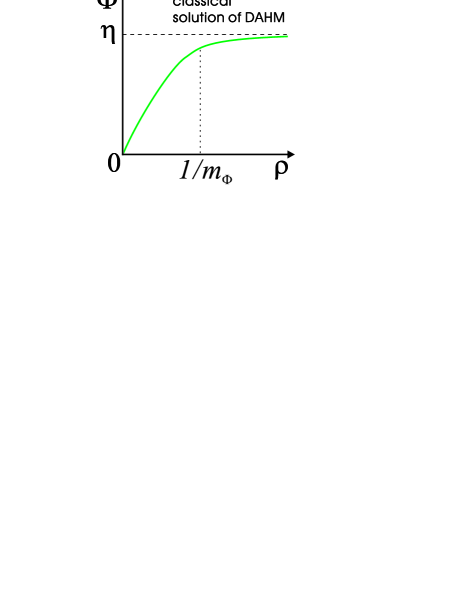
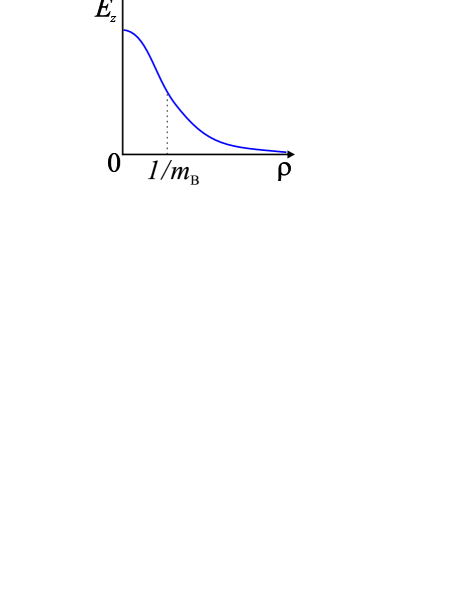
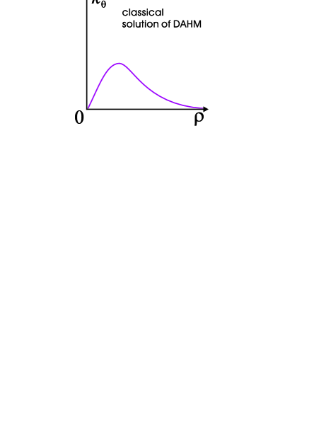
(a)	(b)	(c)

Figure 1: The qualitative behavior of (a) the monopole condensate $\Phi$, (b) the electric field $E_{z}$ and (c) the magnetic current component $k_{\theta}$ around the center of the string as functions of the transverse distance $\rho$. The string is given by a classical solution of the DGL model.

Summarizing, the value of the monopole current near the QCD string (obtained from the classical equations of motion) is zero in the center of the string and it is also zero far from the string. The current has a maximum at a certain distance (which is numerically found to be about $0.2$ fm in the DLG corresponding to SU(2) gluodynamics bali98 ; ref:string:MA:gauge ). The only non–zero component of the classical monopole current is the angle component $k_{\theta}$, while other components (radial, temporal and $z$-component) are zero, $k_{r}=0$, $k_{4}=0$ and $k_{3}=0$.

II.2 Monopole density around QCD string

In the numerical calculations the distributions of the monopole current around the QCD string $\Sigma$ is measured with the help of the correlation function

$$k^{\mathrm{string}}_{\mu}={\langle k_{\mu}(0)\rangle}_{\Sigma}\equiv\frac{\langle k_{\mu}(0)W_{\cal C}\rangle}{\langle W_{\cal C}\rangle}\,,\qquad\partial\Sigma={\cal C}\,,$$ (16)

where $\Sigma$ denotes the string world-sheet corresponding to the minimal surface spanned on the Wilson contour ${\cal C}$. The expectation value (16) is non-zero contrary to Eq.(49) due to the broken Lorenz invariance because of the presence of the string.

The monopole density is non-zero in the absence of the string. We call this value of the density as ”vacuum monopole density”, $|k^{\mathrm{vac}}|$. There are two contributions to this monopole density coming from (i) the long (infrared) monopole loop which forms the monopole condensate ref:Hart ; ref:Zakharov and from (ii) the small monopole loops which represent the perturbative (ultraviolet) fluctuations.

Very naively, the presence of the string should make the monopole density bigger: the vacuum contribution gets an additional contribution coming from the classical (solenoidal) current $k^{\mathrm{class}}\equiv k^{\mathrm{string}}$. The naive picture is plotted in Fig. 2.

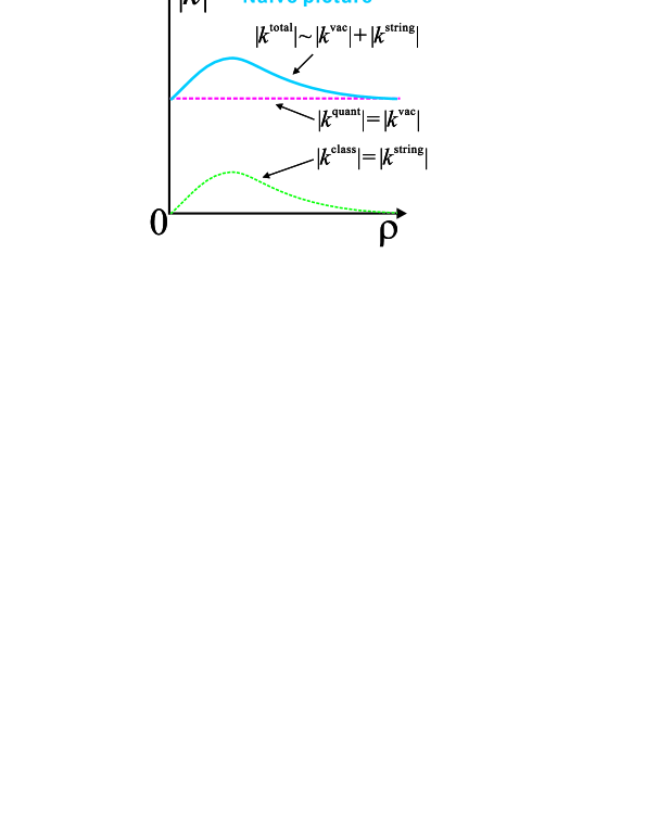
Figure 2: The naive qualitative behavior of the density of monopoles around the QCD string.

Thus, naively, the density of the monopoles should increase at some distance from the string. Moreover, naively one expects that at large transverse distance $\rho$ from the string the monopole density, [according to Eqs. (7,13,14,15)] is controlled by the penetration length since $|k^{\mathrm{string}}|=|k^{\mathrm{vac}}|+\mathrm{const}\,\exp\{-m_{B}\rho\}$.

However, the described qualitative picture definitely contradicts  the numerical results obtained in Ref. ref:monopole:density . In order to investigate the behavior of the monopole density near the QCD string we study analytically the London limit in the next subsection.

II.3 Monopole density in the vicinity of QCD string in the London limit

The London limit is characterized by the infinitely deep potential, $m_{\Phi}\to\infty$. The Lagrangian of the DGL model (1) in this case is

$${\cal L}^{\mathrm{London}}_{DGL}=\frac{1}{4}\,{(\partial_{[\mu,}B_{\nu]})}^{2}+\frac{\eta^{2}}{2}{(\partial_{\mu}\varphi+g\,B_{\mu})}^{2}\,.$$ (17)

The QCD string $\Sigma$ manifests itself as a singularity in the phase of the Higgs field:

$$\partial_{[\mu,}\partial_{\nu]}\varphi(x) = 2\pi{}^{*}\Sigma_{\mu\nu}(x)\,,\quad$$

$${}^{*}\Sigma_{\mu\nu} = \frac{1}{2}\epsilon_{\mu\nu\alpha\beta}\Sigma_{\alpha\beta}(x)\,,$$ (18)

where the string $\Sigma$ is parameterized by the vector ${\bar{x}}_{\mu}(\tau_{1},\tau_{2})$ which depends on the parameters $\tau_{1,2}$. The antisymmetric string current $\Sigma_{\mu\nu}$ is given by the following expression:

$$\Sigma_{\mu\nu}(x)=\int{\mathrm{d}}^{2}\tau\,\frac{\partial{\bar{x}}_{[\mu,}\partial{\bar{x}}_{\nu]}}{\partial\tau_{1}\partial\tau_{2}}\delta^{(4)}(x-{\bar{x}})\,.$$ (19)

The partition function of the model (17) can be rewritten as a sum over the closed strings  ref:Akhmedov :

$${\cal Z} = \int^{\pi}_{-\pi}{\mathrm{D}}\varphi\int_{-\infty}^{\infty}{\mathrm{D}}B\,\exp\Bigl{\{}-\int{\mathrm{d}}^{4}{\cal L}^{\mathrm{London}}_{DGL}(B,\varphi)\Bigr{\}}$$ (20)

$$= \int_{\partial\Sigma=0}{\mathrm{D}}\Sigma\,\exp\bigl{\{}-S_{\mathrm{str}}(\Sigma)\bigr{\}}\,,$$

where $S_{str}$ is the string action:

$$S_{\mathrm{str}}(\Sigma)=$$

$$2\pi^{2}\eta^{2}\int{\mathrm{d}}^{4}x\int{\mathrm{d}}^{4}y\,\Sigma_{\mu\nu}(x)D_{m_{B}}(x-y)\Sigma_{\mu\nu}(y)\,,$$ (21)

and $D_{M}$ is the propagator of the massive scalar particle, $(-\partial^{2}+M^{2})D_{M}(x)=\delta^{(4)}(x)$. The strings are closed: $\partial_{\nu}\Sigma_{\mu\nu}=0$. The derivation of the right hand side in Eq. (20) is easy to make by fixing the unitary gauge, $\varphi=0$ and, consequently, making the shift $B_{\mu}\to B_{\mu}-(1/g)\partial_{\mu}\varphi$. Then Eq. (18) implies that under the shift $\partial_{[\mu,}B_{\nu]}\to\partial_{[\mu,}B_{\nu]}-(2\pi/g){}^{*}\Sigma_{\mu\nu}$. Finally, having integrated over the Gaussian field $B_{\mu}$ we get the right hand side in Eq. (20).

The sources of the electric flux (i.e., the quarks) running along the trajectory ${\cal C}$ are introduced with the help of the Wilson loops written in terms of the original gauge fields $A_{\mu}$. The quantum average of the Wilson loop $W_{\cal C}$ can be rewritten as a sum over the strings similarly to Eq. (20):

$$\langle W_{\cal C}\rangle=$$

$$\frac{1}{{\cal Z}}\int_{\partial\Sigma=j^{\cal C}}{\mathrm{D}}\Sigma\,\exp\bigl{\{}-S_{\mathrm{str}}(\Sigma)-S_{\mathrm{current}}(j^{\cal C})\bigr{\}}\,,$$ (22)

where the strings are spanned on the current $j_{\cal C}$: $\partial_{\nu}\Sigma_{\mu\nu}=j^{\cal C}_{\mu}$. The action for the currents is given by the short-ranged exchange of the dual gauge boson:

$$S_{\mathrm{current}}(j_{\cal C})=$$

$$\frac{e^{2}}{2}\int{\mathrm{d}}^{4}x\int{\mathrm{d}}^{4}y\,j^{\cal C}_{\mu}(x)D_{m_{B}}(x-y)j^{\cal C}_{\mu}(y)\,,$$ (23)

where $e=2\pi/g$ is the electric charge.

Below we evaluate the density of the monopole current in the vicinity of the fixed QCD string. To this end we assume that the leading contribution of the QCD string is naturally given by the minimal surface configuration. Moreover, to avoid boundary (quark) effects, we place the static quarks at the (spatial) infinities of the axis $x_{3}$. Consequently, the quark term (23) does not play any role in the forthcoming discussion.

Thus, we consider the infinite static string which is placed along the third direction. The corresponding string current – calculated from Eq. (19) – is given by the equation:

$$\Sigma_{\mu\nu}=\Bigl{(}\delta_{\mu,3}\delta_{\mu,4}-\delta_{\nu,3}\delta_{\nu,4}\Bigr{)}\delta(x_{1})\delta(x_{2})\,.$$ (24)

The monopole current (6) in the London limit is

$$k_{\mu}=\eta^{2}(\partial_{\mu}\varphi+gB_{\mu})\,.$$ (25)

Let us consider the following generating functional:

$${\cal Z}[\Sigma,C]=\int_{-\infty}^{\infty}{\mathrm{D}}B\,$$

$$\times\,\exp\Bigl{\{}-\int{\mathrm{d}}^{4}x\,\Bigl{[}{\cal L}^{\mathrm{London}}_{DGL}(B,\varphi_{\Sigma})-ik_{\mu}C_{\mu}\Bigr{]}\Bigr{\}}\,,$$ (26)

where the singular phase $\varphi_{\Sigma}$ corresponds to the string position $\Sigma$ fixed via Eq. (18). The monopole current in the presence of the string is given by the variational derivative:

$${\langle k_{\mu}(x)\rangle}_{\Sigma}=\frac{1}{{\cal Z}[\Sigma,0]}\,\frac{\delta}{i\delta C_{\mu}(x)}{\cal Z}[\Sigma,C]{\Bigl{|}}_{C=0}\,.$$ (27)

Analogously, the (squared) monopole density is

$${\langle k^{2}_{\mu}(x)\rangle}_{\Sigma}=\frac{1}{{\cal Z}[\Sigma,0]}\,{\Bigr{(}\frac{\delta}{i\delta C_{\mu}(x)}\Bigr{)}}^{2}{\cal Z}[\Sigma,C]{\Bigl{|}}_{C=0}\,.$$ (28)

Proceeding similarly to the derivation along Eqs.(20,22) we get the following expression for the generating functional:

$${\cal Z}[\Sigma,C]$$ (29)

$$= \exp\Bigl{\{}-\int{\mathrm{d}}^{4}x\int{\mathrm{d}}^{4}y\,\Bigl{[}\frac{g^{2}\eta^{4}}{2}C_{\mu}(x)D^{m_{B}}_{\mu\nu}(x-y)C_{\nu}(y)$$

$$- 2\pi i\eta^{2}C_{\mu}(x)D^{m_{B}}_{\mu\nu}(x-y)\partial_{\alpha}{}^{*}\Sigma_{\alpha\nu}(y)\Bigr{]}-S_{\mathrm{str}}(\Sigma)\Bigr{\}}\,,$$

where $D^{m}_{\mu\nu}(x)$ is the propagator of the massive vector boson $B_{\mu}$, and the string action is given in Eq. (21).

An evaluation of the vacuum expectation value of the monopole density (27) gives:

$$k^{\mathrm{string}}_{\mu} \equiv \langle k_{\mu}\rangle_{\Sigma}$$ (30)

$$= -2\pi\eta^{2}\int{\mathrm{d}}^{4}y\,D^{m_{B}}_{\mu\nu}(x-y)\partial_{\alpha}{}^{*}\Sigma_{\alpha\nu}(y)\,.$$

In particular, in the case of the static string (24) we get the classical London solution:

$$k^{\mathrm{string}}_{i} = -2\pi\eta^{2}\epsilon_{ij}\frac{x_{j}}{\rho}\frac{\partial}{\partial\rho}D^{(2D)}_{m_{B}}(\rho)\,,\quad i,j=1,2\,,\quad$$

$$k^{\mathrm{string}}_{3} = 0\,,\quad k^{\mathrm{string}}_{4}=0\,,$$ (31)

where

$$D^{(2D)}_{m_{B}}=\frac{1}{2\pi}K_{0}(m_{B}\rho)\,.$$ (32)

is the propagator for a scalar massive particle in two space-time dimensions. Using Eqs.(31,32) we get the explicit form of the only non-zero component of the solenoidal current:

$$k^{\mathrm{string}}_{\theta}=\eta^{2}m_{B}K_{1}(m_{B}\rho)\,.$$ (33)

The monopoles form a solenoidal current which circulates around the string in transverse directions.

The squared monopole density is:

$$\langle k^{2}_{\mu}\rangle_{\Sigma}=\langle k_{\mu}\rangle_{\Sigma}^{2}+\langle k^{2}_{\mu}\rangle_{0}\,,$$ (34)

where

$$(k^{\mathrm{quant}}_{\mu})^{2} \equiv \langle k^{2}_{\mu}\rangle_{0}=g^{2}\eta^{4}D^{m_{B}}_{\mathrm{reg}}(0)$$ (35)

$$= \frac{g^{2}\eta^{4}\Lambda^{2}}{16\pi^{2}}+O\bigl{(}\log(\Lambda/m_{B})\bigr{)}$$

is the quantum vacuum correction. We have regularized the divergent expression of the vacuum correction by the momentum cutoff $\Lambda$. The correction is quadratically divergent.

The total (squared) density of the monopole current is given by

$$\langle k^{2}_{\mu}\rangle_{\Sigma} = \eta^{4}M^{2}_{B}K^{2}_{1}(m_{B}\rho)$$ (36)

$$+\frac{g^{2}\eta^{4}\Lambda^{2}}{16\pi^{2}}+O\bigl{(}\log(\Lambda/m_{B})\bigr{)}\,,$$

where the solenoidal current $k^{\mathrm{string}}$ in the London limit is given by Eq.(31). This expression is the exact in the London limit (up to logarithmically divergent but distance-independent corrections).

One may easily see from Eq. (36) that the naive expectation of the density behavior – shown in Fig. 2 – is, in fact, correct in the London limit. Then the total density (in which the coherence length is zero) must have a maximum at the distance of the order of the penetration length, $1/m_{B}$. However, the naive picture depicted in Fig. 2 is not valid the case of the finite coherence length considered below.

II.4 Monopole density in the vicinity of QCD string for finite coherence length

Here we show, that in the real case os a finite coherence length, the naive picture, described in the previous Subsection, is no more correct. Indeed, in this case the value of the monopole condensate is varying in the vicinity of the string, and the (qualitative, at least) generalization of Eq. (36) should read as follows:

$$\langle k^{2}_{\mu}\rangle_{\Sigma} \equiv (k^{\mathrm{string}}_{\mu})^{2}+(k^{\mathrm{quant}}_{\mu})^{2}$$ (37)

$$= (k^{\mathrm{string}}_{\mu})^{2}+\frac{g^{2}|\Phi(\rho)|^{4}\Lambda^{2}}{16\pi^{2}}+\dots\,,$$

where we have taken into account the behavior of the monopole condensate by the simple replacement  $\eta\to|\Phi(\rho)|$ in

$$(k^{\mathrm{quant}}_{\mu})^{2}\equiv\langle k^{2}_{\mu}\rangle_{0}=\frac{g^{2}|\Phi(\rho)|^{4}\Lambda^{2}}{16\pi^{2}}+\dots\,.$$ (38)

Note that the quantum correction to the squared monopole current in the vicinity of the string (with $\rho\sim\xi$) is not equal to the vacuum expectation value measured far outside the string ($\rho\gg\xi$)!

The quantum correction is much stronger than the classical one, therefore the leading behavior of the total density is controlled by the quantum corrections. The behavior of the monopole density in the vicinity of the string is shown in Fig. 3 by the solid line.

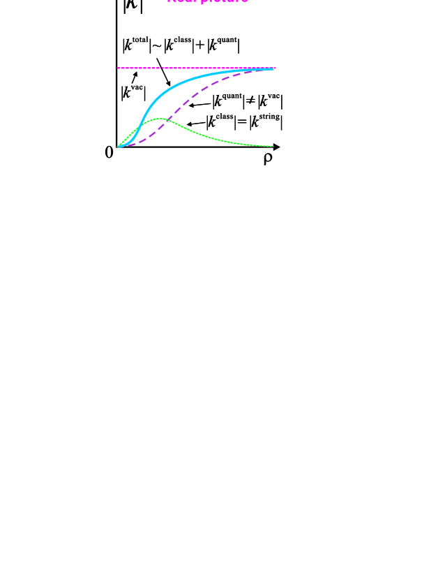
Figure 3: The real qualitative behavior of the density of monopoles around the QCD string.

The various contributions to the total density are also shown in this Figure (the dashed lines). The theoretical expectation – shown in Fig. 3 – is in agreement with the numerical result of Ref. ref:monopole:density .

Thus, we expect that the quantum corrections play an essential role in the case of a finite coherence length. Moreover, the leading behavior of the monopole density at large distances is controlled by the coherence length $\xi$ (and not by the penetration length $\lambda$). This fact can be seen from Eqs. (13,14,15) in the limit $\rho\gg\xi$:

$$\langle|k|\rangle_{\Sigma}(\rho) \sim {\bigl{(}\langle k^{2}_{\mu}\rangle_{\Sigma}\bigr{)}}^{1/2}(\rho)$$ (39)

$$= \frac{g^{2}\Lambda^{2}}{16\pi^{2}}\Biggl{[}1-4\sqrt{\frac{\pi\xi}{2\rho}}\,e^{-\rho/\xi}\Biggr{]}+\dots\,.$$

As it is discussed in Section III, the monopole density should locally be correlated with the condensate $A^{+}A^{-}$ (one can naturally expect a correlation with a short length scale of the order of 0.05fm – this topic will be discussed in the next Section). Therefore, the correlation of the monopole density with the QCD string (39) indicates that the $A^{+}A^{-}$ condensate is also correlated with the QCD string. The correlation lengths for the ”monopole density”–”string” correlations and for the ”$A^{+}A^{-}$ condensate”–”string” correlations should be the same and equal to the coherence length of the dual superconductor:

$$\frac{\langle A^{+}_{\mu}(\rho)A^{-}_{\mu}(\rho)\rangle_{\Sigma}}{\langle A^{+}_{\mu}(\rho)A^{-}_{\mu}(\rho)\rangle_{0}}=1-{\mathrm{const}}\cdot e^{-\rho/\xi}+\dots\,.$$ (40)

with $\rho\gg\xi$. This is the main result of this Section.

III $A^{+}A^{-}$ condensate and Abelian monopole in MA gauge

The MA gauge is defined by the maximization of the functional

$$R[U]=\sum_{l}R_{l}[U]\,,\qquad R_{l}[U]=\frac{1}{2}{\mathrm{Tr}}\Bigl{[}U_{l}\sigma_{3}U_{l}^{\dagger}\sigma_{3}\Bigr{]}\,,$$ (41)

with respect to the gauge transformations,

$$\max_{\Omega\in SU(2)}R[U^{\Omega}]\,,\qquad U^{\Omega}_{x,\mu}=\Omega^{\dagger}_{x}U_{x,\mu}\Omega_{x+\hat{\mu}}\,.$$ (42)

Using the standard parameterization of the $SU(2)$ link matrices,

$$U_{l}=\left(\begin{array}[]{ll}\cos\phi_{l}\,e^{i\theta_{l}}&\sin\phi_{l}\,e^{i\chi_{l}}\\ -\sin\phi_{l}\,e^{-i\chi_{l}}&\cos\phi_{l}\,e^{-i\theta_{l}}\\ \end{array}\right)\,,$$ (45)

we obtain $R_{l}[U]=\cos 2\phi_{l}$. The maximization makes $\phi$ as close to zero as possible.

The off-diagonal fields, $U^{\pm}_{l}=\pm\sin\phi_{l}\,e^{\pm i\chi_{l}}$ correspond to continuum fields $\pm A^{\pm}_{\mu}(x)$ and continuum quantity $A^{+}_{\mu}(x)A^{-}_{\mu}(x)$ corresponds to the lattice quantity $\sin^{2}\phi_{l}\equiv(1-R_{l}[U])/2$. Thus we are able to make an identification (no summation over $\mu$ is assumed):

$$A^{+}_{\mu}(x)A^{-}_{\mu}(x)=\frac{1}{2}\bigl{(}1-R_{x,\mu}[U]\bigr{)}\,,$$ (46)

where the equality is exact in the naive continuum limit.

The first measurements of the local correlation between monopoles and the quantity $R_{l}$ were done in Ref. ref:ambiguity , where the quantity $R_{c}$ was used:

$$R_{c}[U]=\sum_{l\in\partial c}R_{l}[U]\,.$$ (47)

The summation is going over all links belonging to the cube $c$. The distribution of the quantity $R_{c}$ at the cubes occupied by monopoles and the cubes, not occupied by monopoles, is observed. It is shown that at the monopole position the quantity $R_{c}$ is generally smaller compared to the same quantity in the empty space. Therefore, the monopoles suppress the quantity $R_{c}$, and, according to Eq. (46), the $A^{+}A^{-}$ condensate is enhanced on monopoles.

One can suggest, that the correlation of the $A^{+}A^{-}$ condensate with the monopole is short ranged. Indeed, the correlation of the monopole with the SU(2) action in the MA gauge is short ranged, with the characteristic correlation length ref:anatomy $\zeta_{\mathrm{Action}}\approx 0.05$fm. Since the SU(2) action involves the off-diagonal components, it seems natural to suggest that the correlation length $\zeta_{\mathrm{cond}}$ of the off-diagonal components of the gluon field $A^{\pm}$ (or, of the $A^{+}A^{-}$ condensate) with the monopoles is not much higher than the $\zeta_{\mathrm{Action}}$. Thus, one can expect that $\zeta_{\mathrm{cond}}\approx\zeta_{\mathrm{Action}}\approx 0.05$fm.

Thus the $A^{+}A^{-}$–monopole density correlation function,

$$C(r)=\frac{\langle|k_{\nu}(0)|A^{+}_{\mu}(r)A^{-}_{\mu}(r)\rangle}{\langle|k_{\nu}(0)|\rangle\langle A^{+}_{\mu}(0)A^{-}_{\mu}(0)\rangle}-1\,,$$ (48)

at large $r$ is an exponentially decaying function with characteristic length scale $\zeta$.

In general there are two types of correlations: along the monopole current $k_{\mu}$ and perpendicular to the monopole current. In Eq. (48) we assume that the distance $\vec{r}$ is perpendicular to the direction of the monopole current, $R_{\mu}k_{\mu}=0$ (i.e., the correlations are studied in the transverse to the monopole current directions). Obviously, due to the scalar nature of the $A^{+}A^{-}$ operator the correlation of this quantity with the monopole current is zero:

$$\langle k_{\nu}(0)A^{+}_{\mu}(r)A^{-}_{\mu}(r)\rangle\equiv 0\,.$$ (49)

IV Numerical results

IV.1 Method

We use an improved gluonic action found by Iwasaki iwasaki which was already implemented in Ref. suzuki05 :

$$S=\beta\left\{C_{0}\!\sum{\mathrm{Tr}}\mbox{(plaquette)}+C_{1}\!\sum{\mathrm{Tr}}\mbox{(rectangular)}\right\}.$$

The mixing parameters are fixed as $C_{0}+8C_{1}=1$ and $C_{1}=-0.331$. We adopt the coupling constant $\beta=1.2$ which corresponds to the lattice distance $a(\beta=1.2)=0.0792(2)$fm. The lattice size is $32^{4}$ and we use around 5000 thermalized configurations for measurements. To get a good signal-to-noise ratio, the APE smearing technique APE is used when evaluating Wilson loops $W(R,T)=W^{0}+iW^{a}\sigma^{a}$. The thermalized vacuum configurations are gauge-transformed in the MA($+$ U1LA) gauge and in the LA gauge. In the LA gauge the functional $\sum_{s,\mu}Tr[U_{\mu}(s)+U_{\mu}^{\dagger}(s)]$ is maximized with respect to all gauge transformations.

IV.2 The MA gauge case

Non-Abelian electric fields are defined from $1\times 1$ plaquette $U_{\mu\nu}(s)=U^{0}_{\mu\nu}(s)+iU^{a}_{\mu\nu}(s)\sigma^{a}$ as done in Ref. bali-94 :

$$E^{a}_{k}(s) \equiv \frac{1}{2}[U^{a}_{4k}(s-\hat{k})+U^{a}_{4k}(s)]$$ (50)

The static quarks are represented by the Wilson loop $W(R,T)$. The measurements of the electric field are mainly done on the perpendicular plane at the midpoint between the quark pair. A typical example is shown in Fig. 4. Note that electric fields perpendicular to the $Q\bar{Q}$ axis are found to be negligible.

Quantity	gauge	Fig.	$\zeta$ [fm]	$c_{1}$	$c_{2}$	$\chi^{2}/d.o.f.$
$\langle W^{3}E^{3}\rangle$	MA + U1LA	4	$0.140(3)$	$0.044(2)$	$0$	$3.06$
$\langle|k_{\mu}|(A^{+}A^{-})_{u}\rangle$	MA	6	$0.0606(9)$	$1.08(3)$	$-0.0103(2)$	$0.003$
$\langle Wk^{2}\rangle$	MA	8	$0.10(1)$	$0.016(7)$	$0.014300(8)$	$1.35$
$\langle W(A^{+}A^{-})_{u}\rangle$	MA	9	$0.094(8)$	$0.04(1)$	$0.40967(2)$	$0.006$
$\langle W(A^{+}A^{-})_{\theta}\rangle$	MA + U1LA	10	$0.106(9)$	$0.12(4)$	$0.49068(4)$	$0.01$
$\langle W^{3}E^{3}\rangle$	LA	14	$0.139(1)$	$0.038(1)$	$0$	$1.88$
$\langle WA^{2}_{\theta}\rangle$	LA	16	$0.118(4)$	$0.09(1)$	$0.74023(4)$	$0.003$

Table 1: The best fit parameters corresponding to the fits of various quantities by the function (51). We indicate the gauge where the quantity is calculated and the figure number where the quantity is plotted. We set $c_{2}=0$ when the best fit value of $c_{2}$ is consistent with zero.

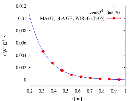
Figure 4: The non-Abelian $\vec{E}$ electric field profile in the MA $+$ U1LA gauge obtained with the use of the $R\times T=6\times 5$ Wilson loop. The solid line denotes the best exponential fit by the function (51) with the best fit parameters given in Table 1.

The correlation length is determined by an exponential fit of the electric field 50 for large $r$ regions, where $r$ is a distance perpendicular to the $Q\bar{Q}$ axis. Below we observe that the electric field as well as other field distributions around the string can be fitted well by a simple exponential function

$$f(r)=c_{1}\exp(-r/\zeta)+c_{2}\,,$$ (51)

where $\zeta$ and $c_{1,2}$ are the fit parameters. The corresponding best fit parameters are presented in Table 1. The best fitting curve for the distribution of the electric field is plotted in Fig. 4 as solid line. From this fit we fix the penetration length $\lambda$.

We show the results for the penetration length in the MA $+$ U1LA gauge in Fig. 5 for various sizes of Wilson loop in space directions $R$. Here we see the penetration lengths for both Abelian $\vec{E}_{A}$ and non-Abelian $\vec{E}$ electric fields are compatible with each other. This is expected, since in MA gauge off-diagonal gluon components are forced to become as small as possible.

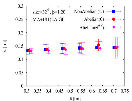
Figure 5: The penetration lengths for non-Abelian $\vec{E}$ and Abelian $\vec{E}_{A}$($\theta$ and $\theta^{AP}$) electric field profiles in the MA $+$ U1LA gauge and their $R$-dependence. Here $\theta$ is defined by $U_{\mu}(s)=\exp(i\theta_{\mu}^{a}(s)\sigma^{a})$ and $\theta^{AP}$ is given in Eq. (45).

Next we study the correlation between the monopole density $\left|k_{\mu}(s)\right|$ and the operator $A^{+}A^{-}(s)$ given by Eq. (46). The correlation data is plotted in Fig. 6. It is completely consistent with the theoretical expectation discussed in Section III. In particular, the scale of correlations between $\left|k_{\mu}(s)\right|$ and $A^{+}A^{-}(s)$ is about $0.06$ fm according to Table 1. This value is pretty close to the scale $\zeta_{\mathrm{Action}}\approx 0.05$fm of the monopole-action correlations.

The histograms of the quantity $R_{c}$, Eq.(47), are plotted in Fig. 7. We discriminate between the histograms obtained at the cubes unoccupied by monopoles and obtained at the cubes occupied by long infrared monopoles. From this figure, we can clearly see the enhancement of the $A^{+}A^{-}$ condensate on the Abelian monopoles.

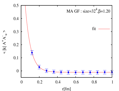
Figure 6: The correlation between the monopole density $|k_{\mu}|$ and the operator $A^{+}A^{-}$ in the MA gauge. The solid line denotes the best exponential fit by the function (51) with the best fit parameters given in Table 1.

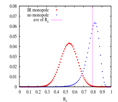
Figure 7: The histogram of the distribution of the quantity $R_{c}$ in Eq.(47) at the locations of infrared monopoles and outside the monopole locations. The vertical line indicates the vacuum average $\langle R_{c}\rangle$.

Let us next derive the coherence length in the MA gauge. The correlations between the Wilson loop and the monopole density, and between the Wilson loop and the quantity $A^{+}A^{-}(s)$ are plotted in Fig. 8 and in Fig. 9, respectively.

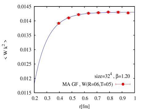
Figure 8: The correlation between the $R\times T=6\times 5$ Wilson loop and the square monopole density in the MA gauge. The solid line denotes the best exponential fit by the function (51) with the best fit parameters given in Table 1.

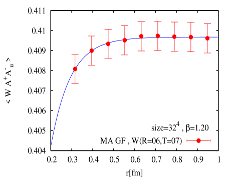
Figure 9: The same as in Fig. 8 but for the correlation between the $R\times T=6\times 7$ Wilson loop and the $A^{+}A^{-}_{u}$ condensate (46).

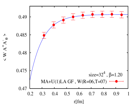
Figure 10: The same as in Fig. 8 but for the correlation between the $R\times T=6\times 7$ Wilson loop and the $A^{+}A^{-}_{\theta}$ condensate (52) in the MA $+$ U1LA gauge.

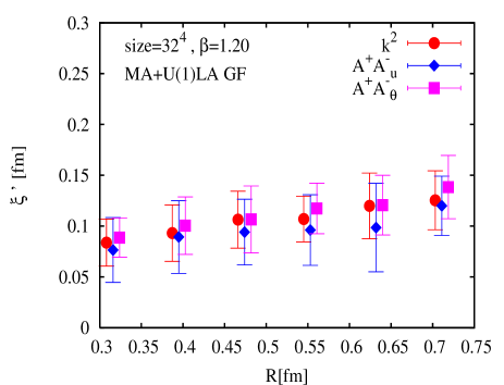
Figure 11: The coherence lengths $\xi^{\prime}$ for $A^{+}A^{-}_{u}$ and $A^{+}A^{-}_{\theta}$ and $k^{2}$ in the MA $+$ U1LA gauge.

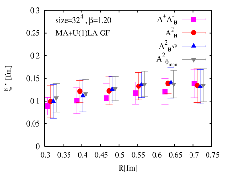
Figure 12: The coherence lengths of dimension 2 gluon operator in the MA $+$ U1LA gauge for various $R$.

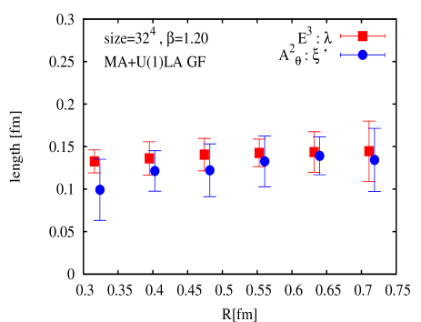
Figure 13: The coherence lengths of dimension 2 gluon operator and the penetration length in MA $+$ U1LA gauge for various $R$.

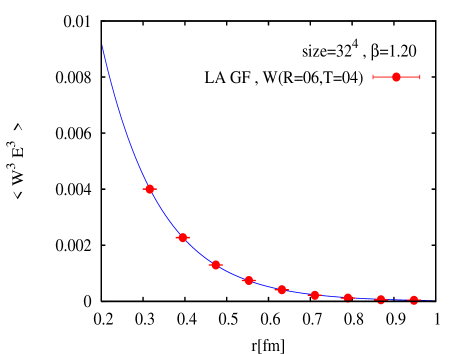
Figure 14: The non-Abelian $\vec{E}$ electric field profile in the Landau gauge obtained with the help of the Wilson loop $W(R\times T=6\times 4)$. The solid line denotes the best exponential fit by the function (51) with the best fit parameters given in Table 1.

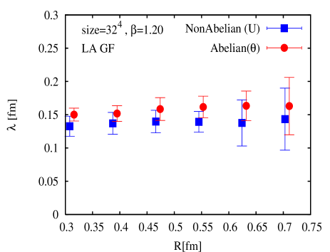
Figure 15: The penetration lengths for the Abelian $\vec{E}_{A}$ and the non-Abelian $\vec{E}$ electric field profiles in the Landau gauge and their dependence on the spatial size $R$ of the Wilson loop.

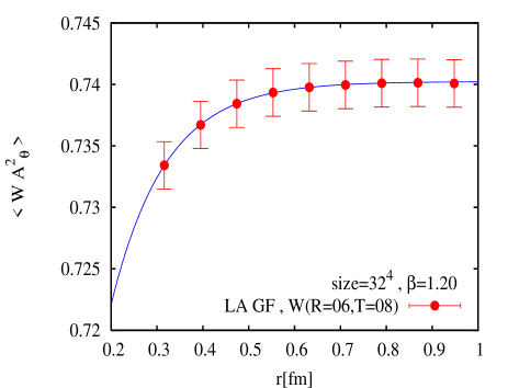
Figure 16: The profiles for the dimension 2 gluon operator in the Landau gauge around $R\times T=6\times 8$ Wilson loop. The solid line denotes the best exponential fit by the function (51) with the best fit parameters given in Table 1.

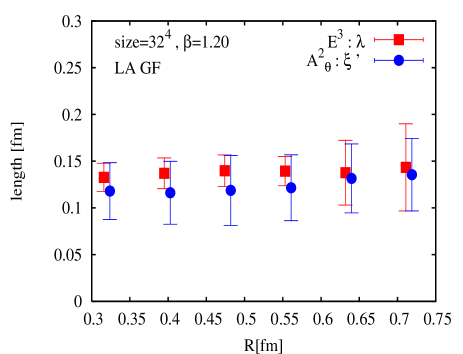
Figure 17: The coherence lengths of the dimension 2 gluon operator and the penetration length in the Landau gauge for various $R$.

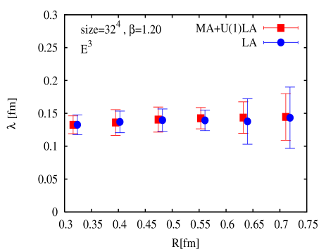
Figure 18: The penetration lengths of the non-Abelian electric field in the Landau gauge and in the MA $+$ U1LA gauge for various $R$.

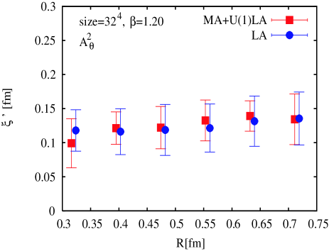
Figure 19: The coherence lengths of the dimension 2 gluon operator in the Landau gauge and in the MA $+$ U1LA gauge for various $R$.

In this gauge, the quantity $A^{+}A^{-}(s)$ may have a physical meaning as we have discussed above. If the remaining $U(1)$ symmetry is gauge fixed by the $U(1)$ Landau gauge, the dimension 2 gluon operator $A^{2}(s)$ also acquires a physical meaning.

In order to study different definitions of the quantity $A^{+}A^{-}(s)$, we plot the profile of the $A^{+}A^{-}(s)$ condensate in Fig. 10 using another definition

$$A^{+}A^{-}_{\theta}=\sum_{s,\mu}\langle\{[\theta^{1}_{\mu}(s)]^{2}+[\theta^{2}_{\mu}(s)]^{2}\}\rangle\,,$$ (52)

which uses the angles $\theta_{\mu}(s)$ given by the relation $U_{\mu}(s)=\exp(i\theta_{\mu}^{a}(s)\sigma^{a})$. In Fig. 11 we show the coherence length determined by the use of the quantities $A^{+}A^{-}_{u}$, $A^{+}A^{-}_{\theta}$ and $k^{2}$. From Fig. 11, we conclude that within the error bars these coherence lengths coincide.

It is interesting to determine a non–perturbative content of the gluon operator. To this end we measure only the monopole contributions to the dimension 2 gluon operator $A^{2}(s)$ after the MA gauge, and, subsequently, the additional $U(1)$ Landau gauge are fixed. This way of defining of the non-perturbative quantities is justified because it is known that in the MA gauge the monopole contributions are responsible for essential non-perturbative physics. The monopole contribution to the coherence lengths is plotted in Fig. 12.

We plot the dependence of the coherence lengths of the spatial extension $R$ of the Wilson loop in Fig. 13. One can clearly see that these values are almost independent on $R$. Moreover, it is very interesting that the values of the coherence lengths are almost the same as those of the penetration lengths. Hence, if this relation holds for larger $R$ – which is very plausible – then the type of the vacuum must be near the border to the type 1 and type 2. This is consistent with the results of Ref. Cea:1995zt ; Singh:1993jj ; matsubara94 ; kato98 obtained with the help of the classical equations of motions of the dual Ginzburg-Landau theory suzuki88 . However it should be emphasized that in this paper the determination of the vacuum type was done for the first time quantum-mechanically.

IV.3 The LA gauge case

The Abelian electric fields $E_{Ai}^{a}$ are defined in the LA gauge similarly to the MA gauge. We use the Abelian plaquettes $\theta_{\mu\nu}^{a}(s)$ defined with the help of the link variables $\theta_{\mu}^{a}(s)$:

$$\theta_{\mu\nu}^{a}(s)\equiv\theta_{\mu}^{a}(s)+\theta^{a}_{\nu}(s+\hat{\mu})-\theta_{\mu}^{a}(s+\hat{\nu})-\theta^{a}_{\nu}(s)$$ (53)

where $\theta_{\mu}^{a}(s)$ is given by $U_{\mu}(s)=\exp(i\theta_{\mu}^{a}(s)\sigma^{a})$.

The dimension 2 gluonic operator is :

$$A^{2}(s)\equiv\sum_{\mu=1}^{4}\sum_{a=1}^{3}\left(\theta_{\mu}^{a}(s)\right)^{2}\,.$$ (54)

First let us discuss a determination of the electric fields around a pair of a static quark and an antiquark in the LA gauge. Since the confining behavior of the chromoelectric string is seen for large enough quark-antiquark distances $R$, we have performed the measurements for various $R$ and $T$. A typical example is shown in Fig. 14.

The $R$ dependence of the penetration lengths is shown in Fig. 15. The maximum quark distance in Fig. 15 is $R=0.71$fm which may not be large enough to see the confining string behavior. On the other hand, we see a small but clear discrepancy between the penetration lengths of the Abelian $\vec{E}_{A}$ and the non-Abelian $\vec{E}$ electric fields. The authors think it is caused by too small distance between the quark and anti-quark so that the different effects from the Columbic interaction may still play a role. Anyway for the interquark distances $R\leq 0.71$ fm, the Abelian dominance is not observed in the LA gauge.

Now let us discuss the measurements of the coherence lengths. As it was explained above, at least in the LA gauge, the operator $A_{\mu}^{2}$ (or its square-root) is physically relevant and may have information about properties of a dual Higgs field characterizing the QCD vacuum. Hence we expect that the coherence length can be measured with the help of $A^{2}(s)$. In Fig. 16 we show a typical example of the $A_{\mu}^{2}$ profile around the string where we have adopted the lattice definition (54) for the operator $A^{2}(s)$. This is very exciting, since the behavior of the profile is just what we expect from a profile of a Higgs field.

We plot the $R$ dependence of the coherence lengths and the penetration lengths in Fig. 17. It is very interesting that the values of the coherence lengths are almost the same as those for the penetration lengths of non-Abelian $\vec{E}$ electric field. Hence if the observed behavior of the correlations is not changed with the increase of $R$, then the type of the vacuum should be fixed to be near the border to the type 1 and type 2 as in MA gauge.

IV.4 Comparison between MA gauge and LA gauge

In order to consider the gauge-(in)dependence of the dual superconductor picture, we show in Fig. 18 the penetration length determined in the MA $+$ U1LA gauge and in the LA gauge. We also plot the coherence length in Fig. 19. From these figures, we observe that the coherence and correlation lengths calculated in different gauges coincide with each other.

V Conclusions

We have observed that

1. The coherence lengths of the vacuum of the SU(2) gluodynamics measured in the Maximal Abelian gauge and in the Landau gauge are all consistent with each other.

2. Since the penetration lengths obtained in the MA gauge are in agreement with the penetration lengths calculated in the LA gauge, we conclude that the type of the vacuum in both gauges is near the border between type 1 and type 2.

3. The monopole contributions to $A^{2}(s)$ alone reproduces the full coherence length, although the absolute value of the correlations is smaller (this last fact is quite natural). Therefore the type of the vacuum can be determined only from the monopole contributions. The observed phenomenon is yet another example of the monopole dominance. It provides an additional support to our expectation that the Abelian monopoles are responsible for all non-perturbative phenomena related to the confinement of color in QCD.

- (1) G. ’t Hooft, in Proceedings of the EPS International Conference, edited by A. Zichichi, p. 1225 (1976).
- (2) S. Mandelstam, Phys. Rept. 23, 245 (1976).
- (3) G. ’t Hooft, Nucl. Phys. B 190, 455 (1981).
- (4) T. Suzuki, Prog. Theor. Phys. 69, 1827(1983).
- (5) A. S. Kronfeld, M. L. Laursen, G. Schierholz, U. J. Wiese, Phys. Lett. B 198, 516 (1987).
- (6) T. Suzuki, I. Yotsuyanagi, Phys. Rev. D42, R4257 (1990);
- (7) T. Suzuki, Nucl. Phys. Proc. Suppl. 30, 176 (1993); M. N. Chernodub, M. I. Polikarpov, in ”Confinement, duality, and nonperturbative aspects of QCD”, Ed. by P. van Baal, Plenum Press, p. 387 (1997).
- (8) G. S. Bali, V. Bornyakov, M. Muller-Preussker, K. Schilling, Phys. Rev. D54, 2863 (1996).
- (9) Y. Koma, M. Koma, E.-M. Ilgenfritz, T. Suzuki, and M. I. Polikarpov, Phys. Rev. D68, 094018 (2003).
- (10) V. Singh D. A. Browne, and R. W. Haymaker, Phys. Lett. B306, 115 (1993).
- (11) H. Shiba, T. Suzuki, Phys. Lett. B351, 519 (1995);
- (12) M. N. Chernodub, M. I. Polikarpov and A. I. Veselov, Nucl. Phys. Proc. Suppl. 49, 307 (1996); M. N. Chernodub, M. I. Polikarpov and A. I. Veselov, Phys. Lett. B 399, 267 (1997); A. Di Giacomo and G. Paffuti, Phys. Rev. D 56, 6816 (1997).
- (13) P. Cea, L. Cosmai, Phys. Rev. D52, 5152 (1995).
- (14) Y. Matsubara, S. Ejiri, T. Suzuki, Nucl. Phys. Proc. Suppl. 34, 176 (1994).
- (15) S. Kato, M. N. Chernodub, S. Kitahara, N. Nakamura, M. I. Polikarpov, T. Suzuki, Nucl. Phys. Proc. Suppl. 63, 471 (1998).
- (16) G. S. Bali, C. Schlichter, K. Schilling, Prog. Theor. Phys. Suppl. 131, 645 (1998).
- (17) T. Suzuki, Prog. Theor. Phys. 80, 929 (1988).
- (18) S. Maedan, T. Suzuki, Prog. Theor. Phys. 81, 229 (1989).
- (19) T. Suzuki, M.N. Chernodub, Phys. Lett. B563, 183 (2003).
- (20) T. Suzuki, K. Ishiguro, Y. Mori, T. Sekido, Phys. Rev. Lett. 94, 132001 (2005); hep-lat/0410039.
- (21) T. A. DeGrand, D. Toussaint, Phys. Rev. D22, 2478 (1980).
- (22) F. V. Gubarev, V. I. Zakharov, ”Gauge invariant monopoles in SU(2) gluodynamics”, hep-lat/0204017; F. V. Gubarev, ”Gauge invariant monopoles in lattice SU(2) gluodynamics”, hep-lat/0204018.
- (23) F. V. Gubarev, S. M. Morozov, ” Condensate, Bianchi Identities and Chromomagnetic Fields Degeneracy in SU(2) YM Theory”, hep-lat/0503023;
- (24) M. N. Chernodub, ”A gauge-invariant object in non-Abelian gauge theory”, hep-lat/0503018;
- (25) M. N. Chernodub, “Yang-Mills theory in Landau gauge as a liquid crystal”, hep-th/0506107; “Liquid crystal defects and confinement in Yang-Mills theory”, hep-th/0507221.
- (26) F. V. Gubarev, L. Stodolsky, V. I. Zakharov, Phys.Rev.Lett. 86, 2220 (2001).
- (27) A. M. Polyakov, Phys. Lett. 59B, 82 (1975); M. E. Peshkin, Ann. Phys. 113, 122 (1978).
- (28) F. V. Gubarev, V. I. Zakharov, Phys. Lett. 501, 28 (2001).
- (29) L. Stodolsky, Pierre van Baal, V. I. Zakharov, Phys. Lett. B552, 214 (2003) and references therein.
- (30) M. J. Lavelle, M. Schaden, Phys. Lett. B208, 297 (1988); M. Lavelle, M. Oleszczuk, Mod. Phys. Lett. A7, 3617 (1992); D. Dudal et al., JHEP 0401, 044 (2004); P. Boucaud et al., Phys. Rev. D66, 034504 (2002); X. Li, C. M. Shakin, ”The Gluon Propagator in Minkowski and Euclidean Space: Role of an Condensate”, hep-ph/0411234 and references therein.
- (31) K-I. Kondo, Phys. Lett. B514, 335 (2001); Phys.Lett. B572, 210 (2003).
- (32) F. V. Gubarev, E. M. Ilgenfritz, M. I. Polikarpov, T. Suzuki, Phys. Lett. B 468, 134 (1999); Y. Koma, M. Koma, E. M. Ilgenfritz, T. Suzuki, Phys. Rev. D 68, 114504 (2003).
- (33) L. M. A. Bettencourt, R. J. Rivers, Phys. Rev. D 51, 1842 (1995).
- (34) A. A. Abrikosov, Sov. Phys. JETP 5, 1174 (1957) [Zh. Eksp. Teor. Fiz. 32, 1442 (1957)].
- (35) H. B. Nielsen, P. Olesen, Nucl. Phys. B 61, 45 (1973).
- (36) A. Hart, M. Teper, Phys. Rev. D 58, 014504 (1998).
- (37) V. G. Bornyakov, P. Y. Boyko, M. I. Polikarpov, V. I. Zakharov, Nucl. Phys. B 672, 222 (2003); M. N. Chernodub, V. I. Zakharov, Nucl. Phys. B 669, 233 (2003) see also discussion in V. I. Zakharov, “Dual string from lattice Yang-Mills theory” hep-ph/0501011.
- (38) V. G. Bornyakov et al. [DIK Collaboration], Phys. Rev. D 70, 074511 (2004).
- (39) See, for example, P. Orland, Nucl. Phys. B 428, 221 (1994); E. T. Akhmedov, M. N. Chernodub, M. I. Polikarpov, M. A. Zubkov, Phys. Rev. D 53, 2087 (1996), and references therein.
- (40) Y. Iwasaki, Nucl. Phys. B258, 141 (1985); Univ. Tsukuba Preprint UTHEP-118(1983) unpublished.
- (41) APE Collaboration: M. Albanese et al., Phys. Lett. B192 163 (1987).
- (42) G. S. Bali, K. Schilling, Ch. Schlichter, Phys. Rev. D51, 5165 (1995).
- (43) S. Hioki, S. Kitahara, Y. Matsubara, O. Miyamura, S. Ohno, T. Suzuki, Phys. Lett. B 271, 201 (1991).
- (44) V. G. Bornyakov, M. N. Chernodub, F. V. Gubarev, M. I. Polikarpov, T. Suzuki, A. I. Veselov, V. I. Zakharov, Phys. Lett. B 537, 291 (2002).