More on the continuum limit of gauge-fixed compact $U(1)$ lattice gauge theory

Abstract

We have verified various proposals that were suggested in our last paper concerning the continuum limit of a compact formulation of the lattice U(1) pure gauge theory in 4 dimensions using a nonperturbative gauge-fixed regularization. Our study reveals that most of the speculations are largely correct. We find clear evidence of a continuous phase transition in the pure gauge theory at ”arbitrarily” large couplings. When probed with quenched staggered fermions with U(1) charge, the theory clearly has a chiral transition for large gauge couplings whose intersection with the phase transition in the pure gauge theory continues to be a promising area for nonperturbative physics. We probe the nature of the continuous phase transition by looking at gauge field propagators in the momentum space and locate the region on the critical manifold where free photons can be recovered.

    PACS: 11.15.Ha; 12.20.Ds

Introduction

The existence and nature of the possible continuum limits of a U(1) theory formulated on the lattice have been a long standing issue in Lattice field theory. QED is arguably the most phenomenologically successful quantum field theory. Nevertheless its behaviour at short distance is still under speculation. The indication from perturbation theory is that, to evade Landau poles QED becomes trivial as one tries to remove the cutoff and interpret it as a fundamental theory (as opposed to an effective theory valid upto some cutoff). The interest in this question is fundamental rather than phenomenological since in QED the landau pole lies beyond the plank scale. The motivation in its resolution stems from the belief that all non-asymptotically free theories are trivial and therefore cannot be fundamental. The existence of QED as a fundamental theory could have a profound impact on the unification schemes [1].

The search for a nontrivial continuum limit for QED on the lattice has not yet borne fruit. With the usual compact pure gauge Wilsonian action there is a confinement-deconfinement phase transition generally understood in terms of monopole condensation [2, 3]. This transition was believed to be first order for a long time but the evidence was inconclusive. A couple of years ago, a high statistics finite size scaling analysis has actually confirmed that the phase transition is indeed first order [4]. With the inclusion of fermions incidentally, this phase transition coincides with a chiral phase transition as well.

The effect of the inclusion of a four-fermi interaction term to the standard Wilson action, both with the compact and non-compact formulations is also being studied for quite some time [5, 6]. Recently in a series of papers [7, 8] it has been concluded that the inclusion of a four-fermi interaction term leads to a continuous chiral phase transition that is distinct from the coulomb-confinement phase transition beyond a certain value of the four-fermi coupling and is actually completely controlled by this coupling. Unfortunately, the study also indicates that the chiral phase transition is logarithmically trivial in conformity with traditional beliefs. An earlier study using the non-compact formulation has yielded similar results [9].

There has also been considerable interest in the search for a continuum limit of QED with nonperturbative properties differing from our familiar QED accessible through perturbation theory. For a review see [10]. Such theories, apart from being interesting by themselves can be useful in the nonperturbative description quantum field theories beyond the standard model.

It has been remarked before that inclusion of fermions to the compact pure Wilson action does not lead to a new phase transition but if scalars are also included, continuum limits with interesting non-perturbative features have been claimed to emerge [11]. One of these continuum limits is associated with a tricritical point where different critical manifolds intersect [11]. Signals of interesting new continuum limits have also been claimed with nonminimal plaquette extensions of the Wilson action [12, 13].

In a previous study [14], we have investigated the continuum limit of a compact formulation of the lattice U(1) gauge theory in 4 dimensions using a novel regularization that was born in the quest for a lattice formulation of chiral gauge theory [15]. This regularization of lattice U(1) theory was originally devised to tame the ’rough gauge’ problem of lattice chiral gauge theories [16]. Because of the lack of gauge-invariance of the lattice chiral gauge theories and the gauge-invariant measure, the longitudinal gauge degrees of freedom (lgdof) couple nonperturbatively to the physical degrees of freedom. To decouple the lgdof which are radially frozen scalar fields, a nonperturbative gauge fixing scheme (corresponding to a local renormalizable covariant gauge fixing in the naive continuum limit) for the compact U(1) gauge fields was proposed. The regularization has a bigger parameter space which apart from the standard Wilson term includes a gauge-fixing term for compact gauge fields and a mass-counterterm. A key feature of this gauge fixing scheme is that the gauge fixing term is not the exact square of the expression used in the gauge fixing condition and as a result not BRST-invariant (as required by Neuberger’s theorem [17] for compact gauge fixing). It has, in addition, appropriate irrelevant terms to make the perturbative vacuum $U_{\mu x}=1$ unique. Because the gauge fixing term obviously breaks gauge invariance, one needs to add counter-terms to restore manifest gauge symmetry.

It has been shown that with the above parameterization, for weak gauge couplings there exists a continuous phase transition (that has been called FM-FMD) at which the lgdof decouple, and the U(1) gauge symmetry is restored [18]. This phase transition has to be accessed from the FM phase since the FMD phase is a phase with broken rotational symmetry.

Our investigations in [14] led to a clear evidence for a continuous phase transition in the pure gauge theory for all values of the gauge couplings studied if the coefficient of the gauge fixing term is kept adequately large. We speculated that the theory will sustain this feature irrespective of how large the gauge coupling is. On the other hand we found that the phase transition is first order if the coefficient of the gauge fixing term small. We naturally assumed that there exists a critical value for the coefficient of the gauge fixing term corresponding to a given gauge coupling, below which the phase transition is first order and is continuous above it. We realized that for a range of gauge couplings this result would be the evidence for the existence of a multicritical line on the FM-FMD interface.

When probed with quenched staggered fermions with U(1) charge, the theory also displayed an unambiguous signal of a chiral transition for large gauge couplings. It seemed to be a likely possibility that the line where the chiral phase transition intersects the FM-FMD transition coincides with the multicritical line where the order of the FM-FMD transition changes. In such an event this multicritical line could become a strong candidate for non-perturbative physics.

In this paper, we have embarked on the task of investigating the truth of the various speculative propositions that were put forth in our exploratory paper [14].

We have confirmed our speculation that indeed if the gauge coupling is increased arbitrarily (numerically, to very large values) the continuous FM-FMD transition is retrieved by adequately increasing the coefficient of the gauge fixing term.

We have also determined the location of the multicritical line precisely as well as the the region where the chiral phase transition meets the FM-FMD transition and we have verified how far they coincide to our precision.

Further in this paper, we have made an effort to probe into the nature of the continuous FM-FMD phase transition by looking at the gauge field propagator in momentum space to see where (if anywhere) in our critical manifold, free photons can be extracted.

The results of our study promises to nurture both the interests, the triviality issue and the possibility of new continuum limits, in lattice $U(1)$ theories.

The Regularization

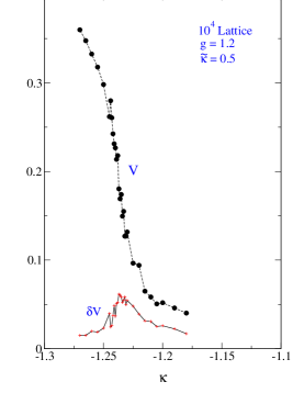
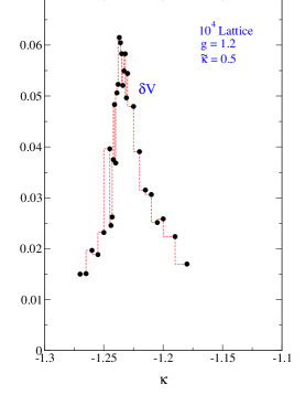
Figure 1: The order parameter $V$ (left) and its fluctuation $\delta V$ (right) as a function of $\kappa$ across the critical point in a region of the FM-FMD interface where the phase transition is continuous. The figure shows the efficiency of the $\delta V$ plot in locating the critical point precisely.

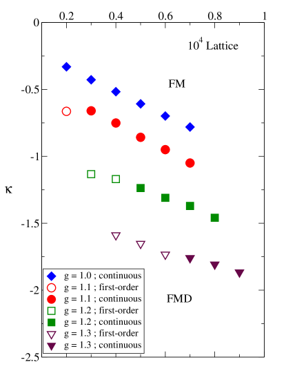
Figure 2: The carefully redetermined FM-FMD phase transition lines in the $\kappa-\tilde{\kappa}$ plane for four different gauge couplings. Hollow symbols represent first-order phase transition and filled symbols represent continuous phase transition. The tricritical line divides the region of hollow symbols from that of filled symbols.

The action for the compact gauge-fixed U(1) theory [15], where the ghosts are free and decoupled, is:

$$S[U]=S_{g}[U]+S_{gf}[U]+S_{ct}[U].$$ (1)

$S_{g}$ is the usual Wilson plaquette action,

$$S_{G}=\frac{1}{g^{2}}\sum_{x\,\mu<\nu}\left(1-{\rm Re}\,U_{\mu\nu x}\right)$$ (2)

where $g$ is the gauge coupling and $U_{\mu x}$ is the group valued U(1) gauge field.

$S_{gf}$ is the BRST-noninvariant compact gauge fixing term,

$$S_{gf}=\tilde{\kappa}\left(\sum_{xyz}\Box(U)_{xy}\Box(U)_{yz}-\sum_{x}B_{x}^{2}\right)$$ (3)

where $\tilde{\kappa}$ is the coefficient of the gauge fixing term, $\Box(U)$ is the covariant lattice Laplacian and

$$B_{x}=\sum_{\mu}\left(\frac{{\cal A}_{\mu,x-\mu}+{\cal A}_{\mu x}}{2}\right)^{2},$$ (4)

where ${\cal A}_{\mu x}{\rm=Im}\,U_{\mu x}$. $S_{gf}$ is not just a naive transcription of the continuum covariant gauge fixing term, it has in addition appropriate irrelevant terms. This makes the action have an unique absolute minimum at $U_{\mu x}=1$, validating weak coupling perturbation theory around $g=0$ or $\tilde{\kappa}=\infty$ and in the naive continuum limit reduces to $1/2\xi\int d^{4}x(\partial_{\mu}A_{\mu})^{2}$ with $\xi=1/(2{\tilde{\kappa}}g^{2})$.

Validity of weak coupling perturbation theory together with perturbative renormalizability helps to determine the form of the counter terms to be present in $S_{ct}$. It turns out that the most important gauge counterterm is the dimension-two counterterm, namely the gauge field mass counterterm given by,

$$S_{ct}=-\kappa\sum_{\mu x}\left(U_{\mu x}+U_{\mu x}^{\dagger}\right).$$ (5)

In the pure bosonic theory there are possible marginal counter-terms including derivatives. However, in the investigation of the gauge-fixed theory as given, the dimension-two counterterm has been mostly considered, because it alone could lead to a continuous phase transition that recovers the gauge symmetry. It was argued that the marginal counter-terms would not possibly create new universality classes for the continuum theory corresponding to large $\tilde{\kappa}$ (for a discussion on other counter-terms, please see [15, 18]).

Numerical Simulation and Results

Confirming our Speculations

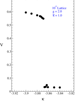
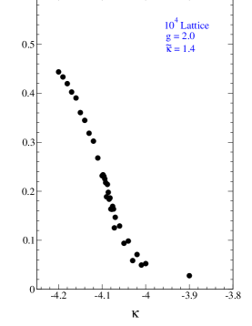
Figure 3: $V$ as a function of $\kappa$ across the critical point at a large value of the gauge coupling (left) in a region of the FM-FMD interface where the phase transition is first-order ( $\kappa_{critical}=-3.868$ ) and (right) in a region of the FM-FMD interface where the phase transition is continuous ( $\kappa_{critical}=-4.084$ ). The figures provide evidence for the existence of the FM-FMD phase transition at a reasonably large gauge coupling.

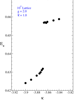
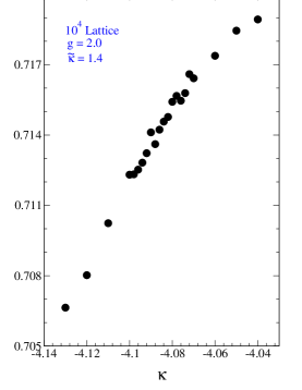
Figure 4: $E_{\kappa}$ as a function of $\kappa$ across the critical point at a large value of the gauge coupling (left) in a region of the FM-FMD interface where the phase transition is first-order ( $\kappa_{critical}=-3.868$ ) and (right) in a region of the FM-FMD interface where the phase transition is continuous ( $\kappa_{critical}=-4.084$ ). The figures provide evidence for the existence of the tricritical point at a reasonably large gauge coupling.

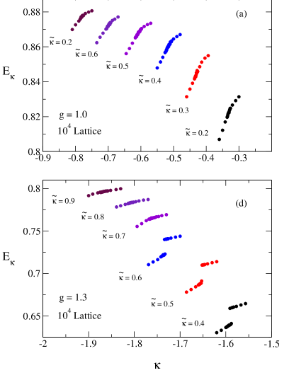
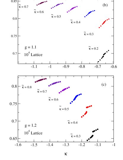
Figure 5: $E_{\kappa}$ as a function of $\kappa$ across the critical points for a range of values of $\tilde{\kappa}$ along the FM-FMD phase transition at four different gauge couplings: (a) g=1.0, (b) g=1.1, (c) g=1.2, and (d) g=1.3. The value of the couplings at which the discrete jump in $E_{\kappa}$ disappear is identified as the tricritical point.

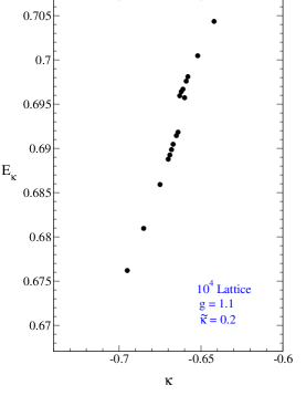
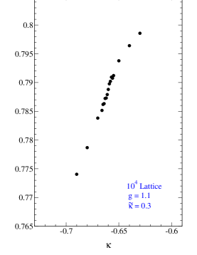
Figure 6: Blow up of $E_{\kappa}$ vs $\kappa$ plot at $g=1.1$ and $\tilde{\kappa}=0.2$ and $0.3$ to show the presence of the minute discrete jump in $E_{\kappa}$ and its disappearance. The critical values of $\kappa$ at $\tilde{\kappa}=0.2$ is -0.664 and at $\tilde{\kappa}=0.3$ is -0.659.

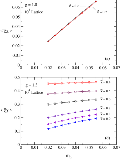
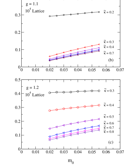
Figure 7: Quenched chiral condensates $\langle\bar{\chi}\chi\rangle$ as a function of the bare fermionic mass $m_{0}$ for a range of values of $\tilde{\kappa}$ along the FM-FMD phase transition at four different gauge couplings: (a) g=1.0, (b) g=1.1, (c) g=1.2, and (d) g=1.3. The values of $\kappa$ have been appropriately chosen to stay close to the critical points. The figures demonstrate the existence of a chiral phase transition and indicate the position where it intersects with the FM-FMD interface.

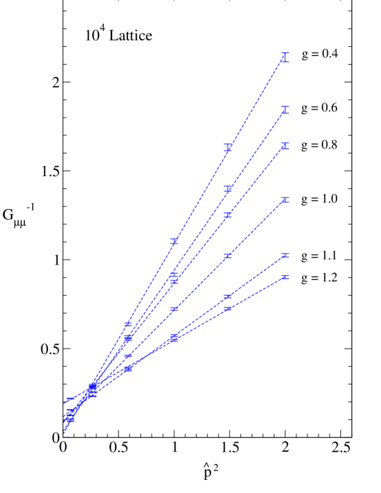
Figure 8: Inverse gauge field propagator $G_{\mu\mu}^{-1}$ in momentum-space as a function of $\hat{p}^{2}$. A straight line with unit slope indicates recovery of free photons.

Since we wanted to find out the order of the phase transition, which is typically inferred from the continuity or discontinuity of some observable at the critical point, the critical points needed to be determined with extreme care and precision in this investigation.

In [14], to obtain the phase diagram of the gauge-fixed pure $U(1)$ theory, given by the action (1), in $(\kappa,\,\tilde{\kappa})$ -plane for fixed values of the gauge coupling $g$, we defined the following observables (for a $L^{4}$-lattice):

$$E_{P} = \frac{1}{6L^{4}}\left\langle\sum_{x,\mu<\nu}{\rm Re}\,U_{\mu\nu x}\right\rangle$$ (6)

$$E_{\kappa} = \frac{1}{4L^{4}}\left\langle\sum_{x,\mu}{\rm Re}\,U_{\mu x}\right\rangle$$ (7)

$$V = \left\langle\sqrt{\frac{1}{4}\sum_{\mu}\left(\frac{1}{L^{4}}\sum_{x}{\rm Im}\,U_{\mu x}\right)^{2}}\;\right\rangle.$$ (8)

where $E_{P}$ and $E_{\kappa}$ though not order parameters, signal phase transitions by sharp changes. We expect $E_{\kappa}\neq 0$ in the broken symmetric phases FM and FMD and $E_{\kappa}\sim 0$ in the symmetric (PM) phase. Besides, $E_{\kappa}$ is expected to be continuous at a continuous phase transition (infinite slope in the infinite volume limit) and show a discrete jump at a first order transition [18, 19]. The true order parameter is $V$ which allows us to distinguish the FMD phase (where $V\neq 0$) from the other phases where $V\sim 0$.

In this paper, in addition to the above observables we have used the fluctuation $\delta V$ in the order parameter $V$ in the determination of the phase diagram. The fluctuation $\delta V$ is expected to display a sharp peak (diverge for the infinite lattice) at the critical point. To show how effective this is, we compare the variation of $V$ and $\delta V$ across the critical point in Fig.1 as an example. Fig.1 clearly demonstrates how by looking at $\delta V$ one can unambiguously determine the critical point (of course for the given lattice).

Throughout this paper error bars have been omitted whenever they are smaller than the symbol size which has been the case more often than not in this study.

The Monte Carlo simulations were done with a 4-hit Metropolis algorithm on a $10^{4}$ lattice. The autocorrelation length for all observables was less than 10 for $10^{4}$ lattices and each expectation value was calculated from one to four thousand independent configurations. The quality of data for each coupling was examined for thermalization before deciding on the number of independent configurations required for measurments at that coupling.

The carefully re-determined phase diagram (FM-FMD phase only), explored in $(\kappa,\tilde{\kappa})$-plane at gauge couplings $g\,=\,1.0,\,1.1,\,1.2,\,1.3$ and 2.0 is shown in Fig.2. There are obviously small deviations to the phase diagram obtained in [14] .However there are no qualitative changes. For each gauge coupling, the FM phase lies above the phase transition and the FMD phase lies below it (i.e, at larger negative values of $\kappa$).

Based on our computation shown in Fig3, in which the variation of $V$ with the coefficient of the counter term $\kappa$ at a reasonably large numerical value of the gauge coupling ($g=2.0$) is shown, we assert that the FM-FMD transition will exist for arbitrarily large values of $g$ provided that the coefficient of the counter term $\kappa$ has a sufficiently large negative value. Moreover this phase transition is continuous if the coefficient of the gauge fixing term $\tilde{\kappa}$ is adequately large (eg: beyond $\tilde{\kappa}\sim 1.2,g=2.0$ ). This is demonstrated in Fig.4 which shows a discrete jump of $E_{\kappa}$ across the critical point at $\tilde{\kappa}=1.0$ as opposed to a continuous change in $E_{\kappa}$ across the critical point at $\tilde{\kappa}=1.4$. This is of course, what we observed in our exploratory paper [14] for gauge couplings upto $g=1.3$ and is in complete agreement with what we had speculated for higher gauge couplings. In determining the tri-critical point, this feature has been investigated in more detail and care in this paper and is discussed below.

To determine the tri-critical points we looked at the variation of the plaquette energy $E_{\kappa}$ with the coefficient of the mass-counterterm $\kappa$ across the FM-FMD phase transition for a range of values of the coefficient of the gauge fixing term ${\tilde{\kappa}}$. This is shown for gauge couplings $g=1.0$ to $g=1.3$, in Figs.5 (a) to (d).

All the figures excepting that for $g=1.0$ exhibit the same feature: A discrete jump of $E_{\kappa}$ at the critical points (implying a first order phase transition) below a particular value for ${\tilde{\kappa}}$ and a continuous change of $E_{\kappa}$ across the critical points (implying a continuous phase transition) above the particular value of ${\tilde{\kappa}}$. For $g=1.0$, $E_{\kappa}$ is always continuous. Where the change of $E_{\kappa}$ is continuous, a hint of a S-shape is visible, a fact which is typical of continuous phase transitions. Please note that the critical point in each $E_{\kappa}-\kappa$ plot is at the middle of the region where the data is most densely packed.

To make the minute jump in $E_{\kappa}$ visible at $g=1.1,\tilde{\kappa}=0.2$ and the subsequent disappearance of the discrete jump at $\tilde{\kappa}=0.3$ we have provided a blow up in Fig.6.

The figures show a clear evidence for the existence of tricritical points which taken together forms a tricritical line cutting across the FM-FMD surface. The tri-critical line starts above $g=1.0$. Note that at $g=1.0$ there is no FM-FMD transition for $\tilde{\kappa}\leq 0.2$. This region belongs to a different phase which has been called PM phase (an uninteresting phase to us which includes the longitudinal gauge degrees of freedom in the continuum) in earlier papers [14, 18].

As we have argued and shown in our last paper [14] the features discussed above are unlikely to be finite size effects since the features become more pronounced as one goes to larger lattices.

We have repeated the calculation for quenched chiral condensates with $U(1)$ charged staggered fermions near our newly determined critical lines. This was done to investigate the possibility of coincidence of the tricritical line mentioned above and the chiral phase transition on the interface between the FM and FMD phases.

We have measured the chiral condensates

$$\langle\bar{\chi}\chi\rangle_{m_{0}}=\frac{1}{L^{4}}\sum_{x}\langle M^{-1}_{xx}\rangle$$ (9)

as a function of vanishing fermionic bare mass $m_{0}$. $M$ is the fermion matrix. The chiral condensates were computed with the Gaussian noise estimator method [20]. Anti-periodic boundary condition in one Euclidean direction is employed.

In Figs.7 (a) to (d), for gauge couplings $g=1.0$ to $g=1.3$, quenched chiral condensates in the FM phase computed at points close to the FM-FMD transition are plotted against the bare mass of staggered fermion $m_{0}$, once again for a range of values of the coefficient of the gauge fixing term $\tilde{\kappa}$, along the FM-FMD critical lines.

Except for $g=1.0$, we see a clear evidence of a chiral phase transition. There exists a critical $\tilde{\kappa}$ for a given gauge coupling $g$ (the third parameter $\kappa$ is used to stay close to the transition), above which the chiral condensates tend towards zero for vanishing fermion mass. Moreover we note, that to our precision the chiral phase transition on the FM-FMD interface coincides with the tricritical line upto $g=1.1$ (at $g=1.0$ there is no tricritical line and no chiral transition). However as the gauge coupling is increased the line of chiral phase transition on the FM-FMD surface appears to move away from the line where the order of the FM-FMD transition changes into the region where the FM-FMD phase transition is continuous.

Nature of the continuum limit

To probe the nature of the continuum limit at the FM-FMD transition, we have studied the gauge field propagator in momentum space to see where (if anywhere) in the critical manifold free photon propagators can be observed. The dimensionless momentum space propagator defined in terms of the group valued gauge fields is

$$G_{\mu\nu}=\frac{1}{g^{2}L^{3}T}\Big{(}\sum_{xy}~{}Im~{}U_{\mu x}~{}Im~{}U_{\nu y}~{}\exp[ip(x-y)]\Big{)}$$ (10)

where $L$ and $T$ are the spatial and temporal extents of the lattice and $p$ are the finite box discrete momenta. This definition obviously is obtained by requiring that

$$\lim_{a\to 0}~{}a^{2}~{}G_{\mu\nu}\longrightarrow\frac{1}{V}\int\int d^{4}xd^{4}y~{}A_{\mu x}~{}A_{\mu y}~{}\exp[ip(x-y)]$$

where $a$ is the lattice spacing, $V$ is the volume and $U_{\mu x}=e^{iagA_{\mu x}}$. We have studied the momentum space propagator $G$ as a function of $\hat{p}^{2}$, $~{}\hat{p}_{\mu}=2\sin(\frac{p_{\mu}}{2})$ being the dimensionless lattice momenta, to see if a $\frac{1}{\hat{p}^{2}}$ dependence can be extracted somewhere on (near) our critical manifold. In a theory for free photons, this is the simplest scheme that can actually be legitimately used to determine the values of the bare couplings in our parameterization.

In our numerical simulation we have actually computed $G_{\mu\mu}$ for different $\mu~{}$ (spatial directions) and averaged over them. A momentum table was set up from where different input momenta were taken corresponding to different values of $\hat{p}^{2}=\sum_{\mu\neq\nu}{\hat{p}_{\nu}}^{2}$. Here ${\hat{p}_{\nu}}$ are the dimensionless finite box discrete momenta. In the end, the inverse of the momentum space gauge field propagator, $G_{\mu\mu}^{-1}$, has been plotted as a function of $\hat{p}^{2}$.

In order to be able to access small momenta, a $6^{3}~{}24$ anisotropic lattice with long temporal extent was used. Calculations were done on $10,000$ configurations and for the errors in $G^{-1}(\hat{p})$, which is a so called biased quantity, Jackknife was employed.

$~{}~{}~{}~{}~{}g~{}~{}~{}~{}~{}~{}$	$~{}~{}~{}~{}~{}~{}\tilde{\kappa}~{}~{}~{}~{}~{}~{}$	$~{}~{}~{}~{}~{}~{}\kappa~{}~{}~{}~{}~{}~{}$	critical $\kappa$
$0.4$	$0.2$	$-0.014$	$-0.064$
$0.6$	$0.3$	$-0.077$	$-0.134$
$0.8$	$0.3$	$-0.169$	$-0.224\leftrightarrow-0.219$
$1.0$	$0.3$	$-0.383$	$-0.433$
$1.1$	$0.5$	$-0.822$	$-0.872$
$1.2$	$0.7$	$-1.348$	$-1.398$

Table 1: Couplings at which the momentum-space gauge field propagator were measured on $6^{3}~{}24$ lattice. The fourth column shows the nearest critical points.

Fig.8 shows $G_{\mu\mu}^{-1}$ as a function of $\hat{p}^{2}$ for gauge couplings $g=0.4,~{}0.6,~{}0.8,~{}1.0,~{}1.1,~{}1.2$. The measurments have been made close to the FM-FMD phase transition from within the FM phase. The values of the critical couplings and the points at which the measurement has been made is listed in Table 1. The figure clearly shows that the dependence of $G_{\mu\mu}^{-1}$ on $\hat{p}^{2}$ is linear for all gauge couplings. However as the gauge coupling grows larger the slope of the straight lines are seen to diminish. Our desired value for the slope $=1$ is obtained between $g=0.4$ and $g=0.6$. So this is where we claim to have recovered free photons. Moreover around $g=0.4$ the intercept on the $G_{\mu\mu}^{-1}$ axis is vanishingly small already on the lattice, indicating that we have actually recovered massless free photons. Our results are consistent with an earlier calculation done at $g=0.4$ [18].

Conclusions and future

Our study with the particular regularization of compact U(1) pure gauge theory with an extended parameter space has confirmed that the speculations made in our last paper [14] were largely correct: We have shown that there is clearly a continuum limit at arbitrarily large gauge couplings provided that the coupling associated with the coefficient of the gauge fixing term is kept adequately large and the coefficient of the mass counter term is sufficiently negative.

We have located the line on the FM-FMD phase transition where its order changes from first to continuous. We have also located the line on the FM-FMD surface where the chiral phase transition intersects. As for the coincidence of these two lines our results appear to have deviated slightly from our speculation. While at smaller gauge coupling (e.g $g=1.0$) the lines clearly coincide, as we move to higher gauge couplings the chiral phase transition seems to move into the region where the FM-FMD transition is continuous (e.g $g=1.3$). Significantly therefore, at large gauge couplings the chiral phase transition on the FM-FMD interface continues to be a strong candidate for non-perturbative physics. However, it is difficult to conclude at our precision level whether the chiral phase transition actually moves into the continuous FM-FMD transition. Even if it does not, the coincidence of the two transitions along the tricritical line is very interesting from the point of view of possible nonperturbative properties of the U(1) theory, as already pointed out in our previous paper [14].

Our momentum space propagator study has revealed that with the continuum limit at the FM-FMD transition, free photons can be recovered at low gauge couplings (in the vicinity of $g=0.4$).

In conclusion, our study of a novel regularization of compact U(1) pure lattice gauge theory reveals that at weak bare gauge coupling, as expected, free photons emerge, while at larger bare couplings the interference of a chiral transition (in this case obtained with U(1) charged quenched fermions) may lead to a continuum limit with interesting nonperturbative properties. With introduction of fermions, the issue of triviality is open for investigation on all continuum limits on the FM-FMD transition.

A major part of the numerical calculations presented in this work is carried out on multiprocessor (Power4 and Power4+) IBM compute machines supported by the 10^th Five Year Plan Project, Theory Division, Saha Institute of Nuclear Physics, under the DAE, Govt. of India.

References

- [1] J.B. Kogut in Strong Coupling Gauge Theories and Beyond, T. Muta and K. Yamawaki, eds, (World scientific, Singapore, 1991) p299; S. Love, ibidem p309, V-A Miransky, Dynamical symmetry breaking in quantum field theories, (World scientific, Singapore, 1993)
- [2] M. Vettorazzo, P. de Forcrand, hep-lat/0311006
- [3] J. Froelich and T. Spencer in Scaling and self similarity in physics, J. Froelich, ed, (Progress in Physics, Birkhauser, 1983) p29
- [4] G. Arnold, T. Lippert and K Schilling Nucl.Phys.(Proc. Suppl) 94 (2001) 651; hep-lat/0011058
- [5] V. Azcoiti, Nucl.Phys.B (Proc. Suppl.)53 (1997) 148; hep-lat/9607070 and references therein
- [6] V. Azcoiti, G. Di Carlo, A. Galante, A. Grillo, V. Laliena, Phys.Lett.B416 (1998) 409; hep-lat/9705014
- [7] J.B. Kogut and C.G. Strouthos, hep-lat/0501003
- [8] J.B. Kogut and C.G. Strouthos, Phys.Rev.D67 (2003) 034504; hep-lat/0211024
- [9] S. Kim, J.B Kogut and M.P.Lombardo, Phys.Lett.B502 (2001) 345; hep-lat/0009029
- [10] J. Jersák, hep-lat/0010014 and references therein
- [11] W. Franzki, C.Frick, J. Jersák and X.Q. Luo, Nucl.Phys.B453 (1995) 355; hep-lat/9505013
- [12] J. Jersák, hep-lat/9801017
- [13] J. Cox, W. Franzki, J. Jersák, C.B. Lang, T. Neuhaus, Nucl.Phys.B532 (1998) 315; hep-lat/9705043
- [14] S. Basak, A.K. De and T. Sinha, Phys.Lett.B580 (2004) 209
- [15] M.F.L. Golterman and Y. Shamir, Phys.Lett.B399 (1997) 148
- [16] W. Bock, M.F.L. Golterman and Y. Shamir, Phys.Rev.Lett 80 (1998) 3444; S. Basak and A.K. De, Phys.Rev.D64 (2001) 014504; S. Basak and A.K. De, Phys.Lett. B522 (2001) 350
- [17] H. Neuberger, Phys.Lett.B183 (1987) 337; M. Testa, Phys. Lett. B429 (1998) 349
- [18] W. Bock, K.C. Leung, M.F.L. Golterman and Y. Shamir, Phys.Rev.D62 (2000) 034507
- [19] W. Bock, M.F.L. Golterman and Y. Shamir, Phys.Rev.D58 (1998) 054506
- [20] K. Bitar, A.D. Kennedy, R. Horsley, S. Meyer and P. Rossi, Nucl.Phys.B313 (1989) 348