The pressure of the $SU(N)$ lattice gauge theory at large–$N$

Abstract

We calculate bulk thermodynamic properties, such as the pressure, energy density, and entropy, in SU(4) and SU(8) lattice gauge theories, for the range of temperatures $T\leq 2.0T_{c}$ and $T\leq 1.6T_{c}$ respectively. We find that the $N=4,8$ results are very close to each other, and to what one finds in SU(3), and are far from the asymptotic free-gas value. We conclude that any explanation of the high-$T$ pressure (or entropy) deficit must be such as to survive the $N\to\infty$ limit. We give some examples of this constraint in action and comment on what this implies for the relevance of gravity duals.

I Introduction

The thermodynamic properties of Quantum Chromodynamics (QCD), besides being of fundamental interest, are currently at the centre of intense experimental research. One of the most interesting phenomena has to do with the range of temperatures, $T$, above the phase transition (or crossover) at $T=T_{c}$, where the theory deconfines and chiral symmetry is restored. Traditionally, the description of this transition assumed that the hadronic phase gives way to a plasma, whose physical degrees of freedom are weakly interacting quarks and gluons. Recent experimental results have, however, challenged this ‘simple’ picture (for example see Heinz (2004) and references therein), and point to a picture of the ‘plasma’ as a very good fluid in the accessible range of $T$ above $T_{c}$. In fact, numerical lattice results had already demonstrated the inadequacy of the simple quark-gluon plasma picture some time ago. Such lattice calculations, both for the pure gauge case Boyd et al. (1996) and with different kinds of fermions Engels et al. (1997), found a large deficit in the pressure and entropy as compared to the Stephan-Boltzmann predictions for a free gluon gas (for pure glue), which remained at the level of more than $10\%$ even at temperatures as high as $T\sim 4T_{c}$. Further evidence that points in the same direction is the survival of hadronic states above $T_{c}$, as seen in recent lattice simulations (for example see Petreczky (2005) and references therein).

These lattice calculations, and more recent experimental observations, have attracted considerable attention (see e.g. Karsch (2002) for a review). Approaches have ranged from modeling the system in terms of noninteracting quasi-particles with the quantum numbers of quarks and gluons but with temperature dependent masses Levai and Heinz (1998); Peshier et al. (1996), to using higher order perturbation theory (restricted by infrared divergences), sometimes including nonperturbative contributions on the dimensionally reduced $3D$ Euclidean lattice Schroder (2004), large re-summations (e.g. Blaizot et al. (2003) and references therein), or, more recently, a description Shuryak and Zahed (2004) in terms of a large number of loosely bound states that survive deconfinement and come in various representations of the gauge and flavor groups, and where one can use for example the lattice masses measured in Petreczky et al. (2002).

In this paper we ask whether this pressure (and entropy) deficit is a dynamical feature not just of SU(3) but of all SU($N$) gauge theories – and in particular whether it survives the $N\to\infty$ limit. In this limit the theory becomes considerably simpler, although not (yet) analytically soluble, and so what happens there should strongly constrain the possible dynamics underlying the phenomenon. For example, in that limit supersymmetric SU($N$) gauge theories become dual to weakly coupled gravity models, and in that context we recall the frequently mentioned prediction Gubser et al. (1998), that the pressure in the strong-coupling limit of the ${\cal N}=4$ and $N=\infty$ supersymmetric gauge theory is $3/4$ of its Stephan-Boltzmann value, which is similar to the deficit, referred to above, that one finds in the non-supersymmetric case.

To address this question we calculate the pressure for $T\leq 2T_{c}$ in $SU(4)$, and $SU(8)$ lattice gauge theories and compare the results to similar SU(3) calculations available in the literature (which we supplement where it is useful to do so). Recent calculations of various properties of SU($N$) gauge theories Teper (2004) have demonstrated that SU(8) is in fact very close to SU($\infty$) for most purposes and have provided information on the location, $\beta_{c}$, of the deconfining transition for various $L_{t}$ and $N$ Lucini et al. (2002, 2004a). Thus our calculations should provide us with an accurate picture of what happens to the pressure at $N=\infty$.

In the next Section we summarise the lattice setup, the relevant thermodynamics, and provide numerical checks that our system is large and homogeneous enough for our thermodynamic relations to be appropriate. We then present our results for the pressure, entropy and related quantities. We discuss the implications of our findings in the concluding section.

II Lattice set up and methodology

The theory is defined on a discretised periodic Euclidean four dimensional space-time with $L^{3}_{s}\times L_{t}$ sites. Here $L_{s,t}$ is the lattice extent in the spatial and Euclidean time directions. The partition function

$$Z(T,V)=\sum_{s}\exp\left\{-\frac{E_{s}}{T}\right\}=\exp\left\{-\frac{F}{T}\right\}=\exp\left\{-\frac{fV}{T}\right\}$$ (1)

defines the free energy $F$ and the free energy density, $f$, and can be expressed as a Euclidean path integral

$$Z(T,V)=\int DU\exp{\left(-\beta S_{\rm W}\right)}.$$ (2)

Here $T=(aL_{t})^{-1}$ is the temperature and $V=(aL_{s})^{3}$ is the spatial volume. When we change $\beta$, so as to change the lattice spacing $a(\beta)$, we change both $T$ and $V$, if $L_{s}$ and $L_{t}$ are kept fixed. In the large–$N$ limit, the ’t Hooft coupling $\lambda=g^{2}N$ is kept fixed, and so we must scale $\beta=2N^{2}/\lambda\propto N^{2}$ in order to keep the lattice spacing fixed in that limit. We use the standard Wilson action $S_{\rm W}$ given by

$$S_{\rm W}=\sum_{P}\left[1-\frac{1}{N}{\rm Re}\text{Tr}\,{U_{P}}\right].$$ (3)

Here $P$ is a lattice plaquette index, and $U_{P}$ is the plaquette variable obtained by multiplying link variables along the circumference of a fundamental plaquette. We perform Monte-Carlo simulations, using the Kennedy-Pendelton heat bath algorithm for the link updates, followed by five over-relaxations of all the $SU(2)$ subgroups of $SU(N)$.

II.1 The method used

In lattice calculations of bulk thermodynamics, one can choose to use either the “integral” method (e.g. Boyd et al. (1996)) or the “differential” method (e.g. Gavai et al. (2005a) or a new variant Gavai et al. (2005b)) or one can attempt a direct evaluation of the density of states (e.g. Bhanot et al. (1987)). We choose to use the first of these methods since the numerical price involved in using larger values of $N$ drives us to smaller $L_{t}$, which means that the lattice spacing is too coarse (about $0.15{\rm fm}$) for the differential method. We have performed preliminary checks for the applicability of the Wang-Landau algorithm Wang and Landau (2001) for the evaluation of the density of states in the $SU(8)$ gauge theory, but found it numerically too costly for the present work.

The properties we will concentrate on are the pressure $p$, the energy density per unit volume $\epsilon$, and the entropy $S$, as a function of temperature. These are given by

$$p = T\frac{\partial}{\partial V}\log Z(T,V)=\frac{T}{V}\log Z(T,V)=-f,$$ (4)

$$\epsilon = \frac{T^{2}}{V}\frac{\partial}{\partial T}\log Z(T,V),$$ (5)

$$\frac{S}{V} = \frac{\epsilon-f}{T}=\frac{\epsilon+p}{T}.$$ (6)

where the second equality in the first and last lines follows if the system is large and homogeneous, i.e. if $V$ is large enough. In addition it is useful to consider the quantity

$$\Delta\equiv\epsilon-3p=T^{5}\frac{\partial}{\partial T}\frac{p}{T^{4}}$$ (7)

which vanishes for an ideal gluon plasma. Again the second equality requires a large enough $V$. To calculate the pressure at temperature $T$ in a volume $V$ with lattice cut-off $a(\beta)$, we express $\log Z$ in the integral form

$$p(T)=\frac{T}{V}\log Z(T,V)=\frac{1}{a^{4}(\beta)L_{s}^{3}L_{t}}\int^{\beta}_{\beta_{0}}d\beta^{\prime}\frac{\partial\log Z}{\partial\beta^{\prime}}$$ (8)

(There is in general an integration constant, but it will disappear when we regularise the pressure later on in this section.) This integral form is useful because it is easy to see from Eqs. (2,3) that

$$\frac{\partial\log Z}{\partial\beta}=-\langle S_{W}\rangle=N_{p}\langle u_{p}\rangle$$ (9)

where $N_{p}=6L_{t}L^{3}_{s}$ is the total number of plaquettes and $u_{p}\equiv{\rm Re}\text{Tr}\,{U_{P}}/N$. So the pressure can be obtained by simply integrating the average plaquette over $\beta$. This pressure has been defined relative to that of the unphysical ‘empty’ vacuum and will therefore be ultraviolet divergent in the continuum limit. To remove this divergence we need to define the pressure relative to that of a more physical system. We shall follow convention and subtract from $p(T)$ its value at $T=0$, calculated with the same value of the cut-off $a(\beta)$. Thus our pressure will be defined with respect to its $T=0$ value. Doing so we obtain from Eq. (9, 8)

$$a^{4}[p(T)-p(0)]=6\int^{\beta}_{\beta_{0}}d\beta^{\prime}(\langle u_{p}\rangle_{T}-\langle u_{p}\rangle_{0}).$$ (10)

where $\langle u_{p}\rangle_{0}$ is calculated on some $L^{4}$ lattice which is large enough for it to be effectively at $T=0$. We replace $p(T)-p(0)\to p(T)$, where from now on it is understood that $p(T)$ is defined relative to its value at $T=0$, and we use $T=(aL_{t})^{-1}$ to rewrite Eq. (10) as

$$\frac{p(T)}{T^{4}}=6L^{4}_{t}\int^{\beta}_{\beta_{0}}d\beta^{\prime}(\langle u_{p}\rangle_{T}-\langle u_{p}\rangle_{0}).$$ (11)

We remark that when our $L_{s}^{3}L_{t}$ lattice is in the confining phase, then $\langle u_{p}\rangle$ is essentially independent of $L_{t}$ and takes the same value as on a $L^{4}_{s}$ lattice (see below). This should become exact as $N\to\infty$ but is accurate enough even for SU(3). Thus as long as we choose $\beta_{0}$ in Eq. (11) such that $a(\beta_{0})L_{t}>1/T_{c}$ then the integration constant, referred to earlier, will cancel.

Finally, we evaluate $\Delta$ in Eq. (7) as follows:

$$\Delta/T^{4} = T\frac{\partial}{\partial T}\frac{p}{T^{4}}$$ (12)

$$= \frac{\partial\beta}{\partial\log T}\frac{\partial}{\partial\beta}\frac{p}{T^{4}}$$ (13)

$$= 6L_{t}^{4}(\langle u_{p}(\beta)\rangle_{0}-\langle u_{p}(\beta)\rangle_{T})\times\frac{\partial\beta}{\partial\log(a(\beta))}.$$ (14)

To evaluate ${\partial\log(a(\beta))}/{\partial\beta}$ we can use calculations of the string tension, $\sigma$, in lattice units. For example, in Lucini et al. (2005a) the calculated values of $a\surd\sigma$ are interpolated in $\beta$ for various $N$ and one can take the derivative of the interpolated form to use in Eq. (14). One could equally well use the calculated mass gap or the deconfining temperature. All these choices will give the same result up to modest $O(a^{2})$ differences.

II.2 Average plaquette

We see from the above that what we need to do is to calculate average plaquettes closely enough in $\beta$ so as to be able to perform the numerical integration in $\beta$. And we need the average plaquettes not only on the $L_{t}L^{3}_{s}$ lattice but also on a reference ‘$T=0$’ $L^{4}$ lattice at each value of $\beta$. However we mostly need values for $\beta\geq\beta_{c}$, where $a(\beta_{c})L_{t}=1/T_{c}$, since $p(T)-p(0)\simeq 0$ once $T<T_{c}$.

We performed calculations in $SU(4)$ on $16^{3}5$ lattices and in $SU(8)$ on $8^{3}5$ lattices for a range of $\beta$ values corresponding to $T/T_{c}\in[0.89,1.98]$ for $SU(4)$, and to $T/T_{c}\in[0.97,1.57]$ for $SU(8)$. Since we use $L_{t}=5$, while the data for $SU(3)$ in Boyd et al. (1996) is for $L_{t}=4,6,8$, we also performed simulations for $SU(3)$ on $20^{3}5$ lattices with $T/T_{c}\in[1,2]$. The results are presented in Tables 1–3.

In addition to the finite $T$ calculations we have performed ‘$T=0$’ calculations on $20^{4}$ lattices for SU(3), and on $16^{4}$ lattices for SU(4). These have the advantage of being on the same spatial volumes as the corresponding finite $T$ calculations, and we know from previous calculations Lucini and Teper (2001); Lucini et al. (2004b) that, for the range of $a(\beta)$ involved, these volumes are large enough to be, effectively, at zero $T$. For SU(8) however, using $8^{4}$ lattices would not be adequate for the largest $\beta$-values, as we will see below. (The same is not true for the finite $T$ calculation on $8^{3}5$ lattices where it is $1/aT$ that sets the scale for finite volume corrections.) We therefore take instead the SU(8) calculations on larger lattices in Lucini et al. (2004b), and interpolate between the values of $\beta$ used there, to obtain average plaquettes at the values of $\beta$ we require. To perform this interpolation we fit with the ansatz

$$\langle u_{p}\rangle_{0}(\beta)=\langle u_{p}\rangle^{P.T.}_{0}(\beta)+\frac{\pi^{2}}{12}\frac{G_{2}}{N\sigma^{2}}(a\sqrt{\sigma})^{4}+c_{4}g^{8}+c_{5}g^{10},$$ (15)

where $\langle u_{p}\rangle^{P.T.}_{0}(\beta)$ is the lattice perturbative result to ${\cal O}(g^{6})$ from Alles et al. (1998) and $N=8$. Our best fit has $\chi^{2}/{\rm dof}=0.93$ with ${\rm dof}=2$, and the best fit parameters are $c_{4}=-6.92$, $c_{5}=26.15$, and a gluon condensate of $\frac{G_{2}}{N\sigma^{2}}=0.72$.

For the scaling of the lattice spacing with $\beta$, needed in Eq. (15) and Eq. (14) and in the temperature scale, we used the interpolation of $a\sqrt{\sigma}$ as a function of $\beta$, as given in Lucini et al. (2005a) . For the temperature scale we need in addition to locate the value of $\beta$ that corresponds to $T=T_{c}$ for the relevant value of $L_{t}$, and for this we have used the values in Lucini et al. (2004a, 2005a). In the case of $SU(3)$ we compared the resulting $T/T_{c}(\beta)$ with that of Boyd et al. (1996) where the physical scale was set by $T_{c}$. We find that the two functions lie on top of each other for $L_{t}=6$. This is consistent with the fact that the $SU(3)$ value of $T_{c}/\sqrt{\sigma}$ for $L_{t}=5,6$ are the same within one sigma Lucini et al. (2004a). This is true for $SU(8)$ as well, where the value of $T_{c}/\sqrt{\sigma}$ for $a=1/(5T_{c})$, and $a=1/(8T_{c})$, are the same within one sigma Lucini et al. (2005a), and we find no point to perform similar comparisons there. For $SU(4)$ the value of $T_{c}/\sqrt{\sigma}$ at $a=1/(5T_{c}),1/(6T_{c})$ is $\sim 5$, and $\sim 3.7$ sigma away from the value at $a=1/(8T_{c})$ Lucini et al. (2005a), which may suggest that in this case $T/T_{c}(\beta)$ at values of $\beta$ that correspond to $T\simeq 8/5T_{c}$ will be smaller when fixing the physical scale with $T_{c}$ rather than with the string tension. Nevertheless the shift between the two is at the level of $\sim 2\%$, and will not change the results presented here. In addition, to fix $T/T_{c}(\beta)$ by fixing $T_{c}$, requires a larger scale calculation of $\beta_{c}(L_{t},L_{s})$ that will include evaluation of finite volume corrections, similar to what was done for $L_{t}=5$ in Lucini et al. (2004a). In view of the small shifts and the high calculational price, we shall ignore this potential ambiguity in this paper.

Table 1: Statistics and results of the Monte-Carlo simulations for $SU(4)$.

$\beta$	$T>0$		$T=0$
	$s_{T}$	(lattice sweeps)$\times 10^{-3}$	$s_{0}$	(lattice sweeps)$\times 10^{-3}$
10.55	0.537478(84)	10	0.537487(81)	5
10.60	0.543862(58)	20	0.543797(25)	15
10.62	0.546212(64)	10	0.546068(33)	10
10.64	0.550279(70)	10	0.548208(16)	20
10.68	0.554213(32)	20	0.552177(16)	20
10.72	0.557649(30)	20	0.555861(14)	20
10.75	0.560051(27)	20	0.558462(13)	20
10.80	0.563923(32)	20	0.562587(16)	20
10.85	0.567592(24)	20	0.566453(17)	20
10.90	0.571107(17)	20	0.570118(16)	20
11.00	0.577707(17)	20	0.576981(11)	20
11.02	0.578985(18)	20	0.578279(11)	20
11.10	0.583911(20)	20	0.583352(12)	20
11.30	0.595398(13)	20	0.595039(10)	20

Table 2: Statistics and results of the Monte-Carlo simulations for $SU(8)$.

$T>0$				$T=0$
$\beta$	$s_{T}$	$L_{s}$	(lattice sweeps)$\times 10^{-3}$	$\beta$	$s_{0}$	(lattice sweeps)$\times 10^{-3}$
43.90	0.525330(80)	14	5	43.85	0.523819(37)	$>20$
43.93	0.526873(79)	8	19.5	44	0.528788(18)	$>20$
44.00	0.531307(50)	10	$>20$	44.35	0.538491(13)	$>20$
44.10	0.534164(34)	12	7	44.85	0.549794(9)	$>20$
44.20	0.536650(70)	14	5	45.7	0.565708(4)	$>20$
44.30	0.539181(30)	8	20
44.45	0.542629(38)	8	30
44.60	0.545812(35)	8	20
44.80	0.549968(37)	8	30
45.00	0.553926(38)	8	20
45.50	0.562992(28)	12	10

Table 3: Statistics and results of the Monte-Carlo simulations for $SU(3)$.

$\beta$	$T>0$		$T=0$
	$s_{T}$	(lattice sweeps)$\times 10^{-3}$	$s_{0}$	(lattice sweeps)$\times 10^{-3}$
5.800	0.568664(100)	10	0.567667(29)	11
5.805	0.569688(153)	20	0.568438(23)	11
5.810	0.570624(55)	10	0.569218(18)	11
5.815	0.571297(81)	10	0.569996(26)	11
5.820	0.572205(78)	10	0.570788(16)	11
5.900	0.583058(38)	10	0.581854(20)	11
6.150	0.609377(27)	10	0.608971(8)	11
6.200	0.613966(31)	10	0.613628(13)	11

II.3 Finite volume effects

For $N=4,8$, one is able to use lattice volumes much smaller than what one needs for $SU(3)$ Boyd et al. (1996). That this is so for the deconfinement transition, has been explicitly demonstrated in Lucini et al. (2004a, 2005a), and is theoretically expected, much more generally, as $N\to\infty$. The main remaining concern has to do with tunnelling between confined and deconfined phases near $T_{c}$. When $V\to\infty$ tunnelling occurs only at $\beta=\beta_{c}$ (in a calculation of sufficient statistics) and the system is in the appropriate pure phase for $T<T_{c}$ and for $T>T_{c}$. On a finite volume, where this is no longer true, one minimises finite-$V$ corrections by calculating the average plaquettes only in field configurations that are confining, for $T<T_{c}$, or deconfining, for $T>T_{c}$. This ensures that the system is as close as possible to being ‘large and homogeneous’ as is required in the derivations of this Section. Because the latent heat grows $\propto N^{2}$ Lucini et al. (2005a) the region $\delta T$ around $T_{c}$ in which there is significant tunnelling shrinks as $\delta T\propto 1/N^{2}$ for a given $V$. Hence we can reduce $V$ as $N$ increases without increasing the ambiguity of the calculation. For SU(3), where the phase transition is only weakly first order, frequent tunneling occurs in the vicinity of $T_{c}$ in the volume we use, and it is not practical to attempt to separate phases. This will smear the apparent variation of the pressure across $T_{c}$ in the case of SU(3).

We now turn to a more detailed discussion of finite volume effects. If $\xi$ is the longest correlation length, in lattice units, in a volume of length $L$, then finite volume effects will be negligible if $\xi\ll L$. In addition finite volume corrections will be suppressed as $N\to\infty$. In our particular context, $\xi$ is given by the inverse mass of the lightest (non-vacuum) state that couples to the loop that winds around the temporal torus. In both the confined and deconfined phases, these masses decrease as $T\to T_{c}$. Therefore the largest length scale is set by the masses at $T=T_{c}$. As $N$ increases these masses increase towards their limits, with $1/N^{2}$ corrections that are quite large Lucini et al. (2005a).

II.3.1 The deconfined phase

In the deconfined phase, on an $L_{s}^{3}\times 5$ lattice at $T=T^{+}_{c}$, the value of $\xi$ is about $12.5$ lattice spacings for $SU(3)$, while it is about $5.2$, and $2.4$ lattice spacings for $SU(4)$, and $SU(8)$ respectively Lucini et al. (2005a). This suggests that our choice of $L_{s}=16$ for SU(4) and $L_{s}=8$ for SU(8) should be adequate. In addition it is known from calculations of $T_{c}$ Lucini et al. (2002, 2004a, 2005a) that on such lattices the tunnelling is sufficiently rare that even at $T=T_{c}$ one can reliably categorise field configurations as confined or deconfined and hence calculate the average plaquette in just the deconfined phase if one so wishes. For our supplementary SU(3) calculations we use $L_{s}=20$ which is much smaller in units of $\xi$. In practice this means that in this case we are unable to separate phases at $T\simeq T_{c}$.

To explicitly confirm our control of finite volume effects, we have compared the SU(8) value of $\langle u_{p}(\beta)\rangle$ as measured in the deconfined phase of the our $8^{3}\times 5$ lattice with other $L_{s}^{3}\times 5$ results from other studies Bringoltz and Teper (2005). As summarised in Table 4, the results are consistent at the $2\sigma$ level.

Table 4: Finite volume effects for plaquette average in the deconfined phase on a $L_{t}=5$ lattice, for $SU(8)$.

$\beta$	$L_{s}=8$	$L_{s}=10$	$L_{s}=12$	$L_{s}=14$
43.95	-	0.529788(100)	0.529944(65)	-
44.00	0.531343(45)	0.531307(50)	-	-
44.10	0.534219(54)	-	0.534164(34)	-
44.20	0.536714(33)	-	0.536689(54)	0.536650(70)
44.25	-	-	0.537954(60)	0.537850(100)
44.30	0.539181(29)	-	-	0.539220(100)
45.50	0.563093(41)	-	0.562992(28)	-

II.3.2 The confined phase

As we remarked above (see below for explicit evidence) we have $\langle u_{p}\rangle_{T}\simeq\langle u_{p}\rangle_{0}$ in the confined phase and so the contribution in Eq. (11) of the range of $\beta$ where the finite $T$ system is confined is very small. Nonetheless, we include an integration over that range for completeness and so we need to discuss possible finite $V$ corrections for this case as well.

In the confined phase, on an $L_{s}^{3}\times 5$ lattice at $T=T^{-}_{c}$, the value of $\xi$ is about $9.5$ lattice spacings for $SU(3)$, but drops to about $5$ and $3.5$ for $SU(4)$ and $SU(8)$ respectively Lucini et al. (2005a). This leaves our choice of $L_{s}$ still reasonable for $SU(4)$ but somewhat worse for SU(8). In Table 5 we provide a finite volume check for the latter case that proves reassuring.

Finally we return to our earlier comment that for the ‘T=0’ $L^{4}$ lattice calculations, a size $L=8$ in SU(8) would not be large enough. This is demonstrated, for our largest $\beta$-value, in Table 6, where we also present the value of $L_{t}\times T/T_{c}(\beta)$ (in our $L_{t}=5$ calculations). In the confined $L_{s}^{4}$ lattice, finite volume effects will be suppressed when the latter is much smaller than $L_{s}$. Clearly for $\beta=45.70$, and $L_{s}=8$, this is not the case.

By contrast, for $SU(4)$ the finite volume effects seems not to be large on the $16^{4}$ lattice as we checked for our largest value of $\beta=11.30$. There the value of the plaquette on a $20^{4}$ lattice is $0.595014(4)$ Lucini and Teper (2001), which is consistent within $\sim 2.3$ sigma with the value presented in Table 1. This is in spite of the fact that for this coupling $L_{t}\times T/T_{c}=10$, and is not so much smaller than $L_{s}=16$.

Table 5: Finite volume effects for plaquette average in the confined phase on a $L_{t}=5$ lattice, for $SU(8)$.

$\beta$	$L_{s}=8$	$L_{s}=10$	$L_{s}=12$	$L_{s}=14$
43.90	0.525750(87)	-	0.525613(54)	0.525425(90)
43.95	-	0.527240(34)	0.527275(48)	0.527280(50)
44.00	-	-	0.528867(33)	0.528810(50)
44.10	-	-	0.531880(45)	0.531900(60)

Table 6: Finite volume effects for plaquette average in the confined phase on a $L^{4}$ lattice, for $SU(8)$. The last column is for $L_{t}=5$.

$\beta$	$L_{s}=8$	$L_{s}=10$	$L_{s}=16$	$L_{t}\times T/T_{c}$
44.00	0.528876(39)	0.528788(18)	-	5.05
45.70	0.566089(23)	-	0.565708(4)	8.20

III Results

To obtain the pressure from the values of the average plaquette presented in Tables 1–3 we need to perform the integration in Eq. (11), which we do by numerical trapezoids. We have already remarked that the contribution to the pressure from the confined phase is negligible. In Table 7 we provide some accurate evidence for this. We show the values of the average plaquette on $L^{4}$ lattices, corresponding to $T\simeq 0$, as well as the values on $L_{s}^{3}5$ lattices at $T\simeq T_{c}$, with the latter obtained separately in the confined and deconfined phases. (These volumes are large enough for there to be no tunnelling, or even attempted tunnelling, within our available statistics.) We see that for both $SU(4)$ and $SU(8)$ there is no visible difference between the plaquette at $T=0$ and $T=T_{c}$ in the confined phase at, say, the $2\sigma$ level. Any difference, (and there obviously must be some difference) is clearly negligible when compared to the difference between the confined and deconfined phases at (and above) $T_{c}$.

Table 7: The plaquette average in the confined phase, $C$, at $T\simeq T_{c}$ compared to the $T=0$ value and to the value in the deconfined phase, $D$. For $SU(4)$ and $SU(8)$.

$\beta$	$N$	$lattice$	$\langle u_{p}\rangle$	$phase$	$T$
10.635	4	$32^{3}5$	0.549563(33)	D	$T_{c}$
		$32^{3}5$	0.547689(11)	C	$T_{c}$
		$10^{4}$	0.547640(27)	C	$0$
43.965	8	$12^{3}5$	0.530352(23)	D	$T_{c}$
		$12^{3}5$	0.527725(27)	C	$T_{c}$
		$10^{4}$	0.527648(24)	C	$0$

In presenting our results for the pressure, we shall normalize to the lattice Stephan-Boltzmann result given by

$$\left(p/T^{4}\right)_{\text{free--gas}}=(N_{c}^{2}-1)\frac{\pi^{2}}{45}\times R_{I}(L_{t}).$$ (16)

Here $R_{I}$ includes the effects of discretization errors in the integral method Engels et al. (2000); Engels (2005). For large values of $L_{t}$, and an infinite volume, it is given by

$$R_{I}(L_{t})=1+\frac{8}{21}\left(\frac{\pi}{L_{t}}\right)^{2}+\frac{5}{21}\left(\frac{\pi}{L_{t}}\right)^{4}+{\cal O}\left(\frac{1}{L_{t}}\right)^{6}.$$ (17)

Since some values of $L_{t}$ discussed in this work are not very large, we shall use the full correction, which includes higher orders in $1/L_{t}$, instead of Eq. (17). This was calculated numerically for the infinite volume limit in Engels et al. (2000) for $L_{t}=4,6,8$, and we supplement this calculation, with the same numerical routines Engels (2005), for other values of $L_{t}$. A summary of $R_{I}(L_{t})$ in the infinite volume limit is given in Table 8.

Table 8: The lattice discretisation errors correction factor $R_{I}(L_{t})$ in the infinite volume limit.

$L_{t}=2$	$L_{t}=3$	$L_{t}=4$	$L_{t}=5$	$L_{t}=6$	$L_{t}=8$
$2.04526(4)$	$1.6913(2)$	$1.3778(1)$	$1.2129(6)$	$1.1323(1)$	$1.0659(1)$

We find that the full correction for $L_{t}=5$ is a $\sim 21\%$ effect, which, without this normalisation, might obscure the physical effects that we are interested in. This is an appropriate normalisation because we expect Eq. (16) to provide the $T\to\infty$ limit of $p/T^{4}$. The same applies to the internal energy density, since $\epsilon\to 3p$ as $T\to\infty$, and so when presenting our results for $\epsilon/T^{4}$ we normalise it with the expression in Eq. (16). For similar reasons we shall use the same normalisation when presenting our results for the entropy. For $\Delta/T^{4}$ it is less clear what normalisation one should use since $\Delta=\epsilon-3p\to 0$ as $T\to\infty$, but for ease of comparison we shall once again normalise using Eq. (16).

To facilitate the comparison of our results with earlier work on SU(3) Boyd et al. (1996), which was done for $L_{t}=4,6,8$, we have performed $SU(3)$ simulations with $L_{t}=5$. The spatial size is $L_{s}=20$ which should be sufficiently large in the light of our above discussion of finite volume effects (and we note that it satisfies an empirical rule that one needs $L_{s}/L_{t}\geq 4$ Engels et al. (1990)).

We present our $N=4$ and $N=8$ results for $p/T^{4}$ in Fig. 1. We also show there our calculations of the $SU(3)$ pressure for $L_{t}=5$, as well as the $L_{t}=6$ calculations from Boyd et al. (1996). Although our errors on the $SU(3)$ pressure are probably underestimated, since the mesh in $\beta$ is quite coarse, nonetheless one can clearly infer that the pressure in the $SU(4)$ and $SU(8)$ cases is remarkably close to that in $SU(3)$ and hence that the well-known pressure deficit observed in SU(3) is in fact a property of the large-$N$ planar theory.

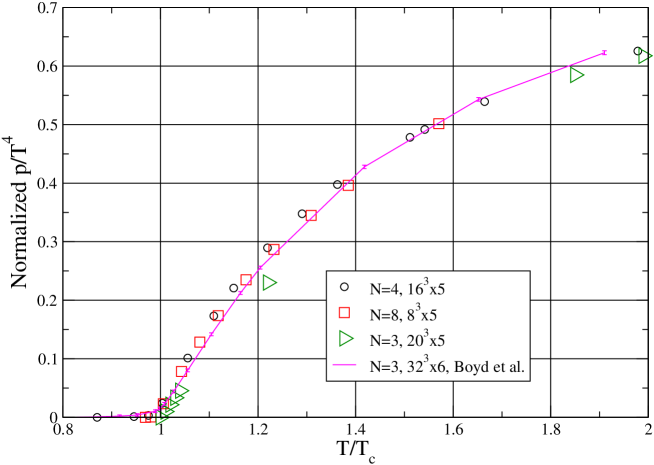
Figure 1: The pressure, normalized to the lattice Stephan-Boltzmann pressure, including the full discretization errors. The symbol’s vertical sizes are representing the largest error bars (which are received for the highest temperature). The solid line is for $SU(3)$ and $L_{t}=6$ from Boyd et al. (1996).

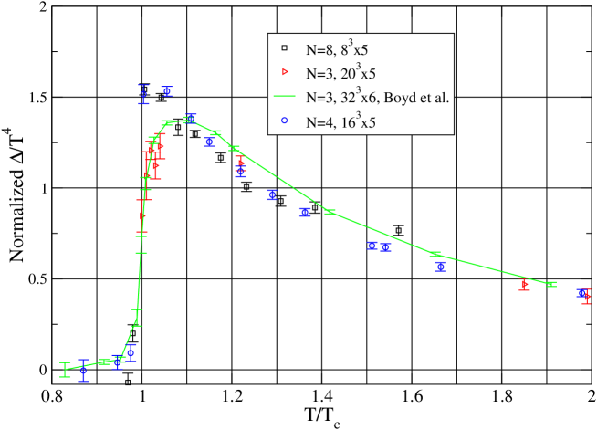
Figure 2: Results for $\Delta(T)/T^{4}=T\frac{\partial p/T^{4}}{\partial T}$, normalized by the same coefficient as we normalize the pressure. The solid line is for $SU(3)$ and $L_{t}=6$ from Boyd et al. (1996).

In Fig. 2 we present our results for $\Delta/T^{4}$ as calculated from Eq. (14). This quantity can be considered as a measure of the interaction and non-conformality of the theory, since it is identically zero both for the noninteracting Stephan-Boltzmann case, and for the ${\cal N}=4$ supersymmetric $SU(N)$ gauge theory. As remarked above, we normalise with the expression in Eq. (16). We also note that in this case there are no errors from a numerical integration, and this enables a fair comparison with the $SU(3)$ data of Boyd et al. (1996). Comparing the results for different $N$ we see that, just as for the pressure, the results for all these gauge theories are very similar.

To see what is the behaviour of $\Delta/T^{4}$ at even higher temperatures, we use the plaquette averages on lattices with $L_{t}=2,3,4,5$, that have been calculated at fixed couplings which correspond to $T\simeq T_{c}$ for $L_{t}=5$ Lucini et al. (2005a). We present the results in Table 9. For the evaluation of $\Delta$ one needs $d\log a/d\beta$ which we present in the table as well.

Table 9: Plaquette average in the deconfined phase for lattice with fixed coupling, at different values of $L_{t}$, and with $\beta$ that corresponds to roughly the deconfining temperature at $L_{t}=5$: $\beta=5.800,10.635,44.00$ for $N=3,4,8$. The data for $L_{t}=5$ are obtained for $L=64,32,10$ for $N=3,4,8$ (for $N=3$, $\delta\langle u_{p}\rangle$ is the difference between the plaquette as calculated within separate confined and deconfined sequences of field configurations).

$N$	$L^{3}\times 5$	$8^{3}\times 4$	$8^{3}\times 3$	$8^{3}\times 2$	$10^{4}$	$-d\log a/d\beta$
3	$\delta\langle u_{p}\rangle=0.00080(5)$	0.570987(37)	0.573311(34)	0.578121(27)	0.567642(29)	2.075(17)
4	0.549563(33)	0.551604(33)	0.554047(27)	0.559163(24)	0.547640(27)	1.440(23)
8	0.531202(92)	0.533066(25)	0.535991(24)	0.541518(17)	0.528788(18)	0.384(20)

In such calculations where one varies $T$ by varying $L_{t}$, the lattice spacing varies as $a=1/L_{t}\times 1/T$ when expressed in units of the relevant temperature scale, and so lattice spacing corrections will vary with $T$.

The resulting values of $\Delta$ in the case of SU(3) are plotted in Fig. 3 where they are compared to the results obtained from calculations where one varies $T$ by varying $\beta$ at fixed $L_{t}$. These calculations include ours for $L_{t}=5$ and those of Boyd et al. (1996) for $L_{t}=4,6$.

As we see from Fig. 3 our $L_{t}=5$ $SU(3)$ results do in fact lie between the $L_{t}=4,6$ results of Boyd et al. (1996) as one would expect. We observe that the $T$ dependence is very similar in all cases, and that the remaining $L_{t}$ dependence appears to be much the same for the different kinds of calculation. This gives us confidence that performing calculations where we vary $T$ by varying $L_{t}$ at fixed $\beta$ does not introduce any unanticipated and important systematic errors.

Having performed this check, we compare in Fig. 4 our results for $\Delta$ in the range $T_{c}\leq T\leq 2.5T_{c}$ that corresponds to $5\geq L_{t}\geq 2$. This comparison confirms what we observed in Fig. 2 over a smaller range of $T$: $\Delta$ is very similar for all the values of $N$ (except very close to $T_{c}$), implying that this is also a property of the $N=\infty$ planar limit.

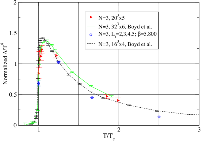
Figure 3: Results for $\Delta(T)/T^{4}=T\frac{\partial p/T^{4}}{\partial T}$, normalized to the free-gas result. The lines are for $SU(3)$ and $L_{t}=4,6$ from Boyd et al. (1996). Red triangles correspond to $L_{t}=5$, and changing $\beta$, while blue circles correspond to changing $L_{t}$ and keeping a fixed $\beta=5.800$.

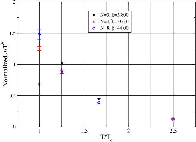
Figure 4: Results for $\Delta(T)/T^{4}=T\frac{\partial p/T^{4}}{\partial T}$ for $N=3,4,8$, by fixing $\beta=\beta_{c}(L_{t}=5)$, while changing $L_{t}=2,3,4,5$.

Finally we present in Fig. 5 our results for the normalized energy density $\epsilon=\Delta+3p$, and the entropy per unit volume $s=(\epsilon+p)/T$. The lines are the $SU(3)$ result of Boyd et al. (1996) with $L_{t}=6$. Again we see very little dependence on the gauge group, implying very similar curves for $N=\infty$.

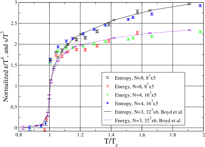
Figure 5: Results for energy density and entropy, normalized to the lattice Stephan-Boltzmann result, including the full discretization errors. The solid line is for $SU(3)$ and $L_{t}=6$ from Boyd et al. (1996).

IV Summary and discussion

In this work we have analyzed numerically the bulk thermodynamics of SU(4) and SU(8) gauge theories. We found that the pressure, when normalized to the Stephan-Boltzmann lattice pressure, is practically the same as for SU(3), in the range $T_{c}\leq T\leq 1.6T_{c}$ that we analyze. We found the same to be the case for the internal energy and entropy, as well as for the quantity $\Delta=\epsilon-3p$ (where we were able to explore temperatures up to $T\simeq 2.5T_{c}$). All this implies that the dynamics that drives the deconfined system far from its noninteracting gluon plasma limit, must remain equally important in the $N=\infty$ planar theory. This is encouraging since that limit is simpler to approach analytically, in particular using gravity duals.

Our results have been (mostly) obtained for lattice spacings $a=1/(5T)$ and it would be useful to perform a larger scale calculation that allows us to perform an explicit continuum extrapolation. However past SU(3) calculations of the pressure, and calculations in SU($N$) of various physical quantities, strongly suggest that our choice of $a$ already provides us with a reliable preview of what such a more complete calculation would produce.

Our results imply that any explanation of the QCD pressure deficit must survive the large–$N$ limit, and so should not be driven by special features particular to SU(3). This can provide a strong constraint on such explanations. For example, in approaches based on higher order perturbation theory, it tells us that the important contributions must be planar. In models focussing on resonances and bound states, it must be that the dominant states are coloured, since the contribution of colour singlets will vanish as $N\to\infty$. Models using ‘quasi-particles’ should place these in colour representations that do not exclude their presence at $N=\infty$, and in fact give them $T$-dependent properties which depend weakly on $N$. Also, topological fluctuations should play no role in this deficit since the evidence is that there are no topological fluctuations of any size in the deconfined phase at large-$N$ Lucini et al. (2005b); Del Debbio et al. (2004).

Finally, we emphasize that our conclusion that the SU(3) pressure and entropy deficits are features of the large-$N$ gauge theory, means that these ‘observable’ phenomena can, in principle, be addressed using AdS/CFT gravity duals. Indeed it is precisely where the deficit is large that the coupling must be strong and this is also precisely where, at large $N$, such dualities can be established. As has been frequently emphasized (see for example Gavai et al. (2005a, b)) the deficit in the normalized entropy is not far from the value of $s/s_{\text{free-gas}}=3/4$ given by the AdS/CFT prediction. In this paper we have found that large-$N$ gauge theories show the same behaviour, as we see in Fig. 5 where, for the entropy, the horizontal line $s_{\text{normalized}}/T^{3}=3$ would correspond to $s/s_{\text{free-gas}}=3/4$. Our results can therefore serve as a bridge between the AdS/CFT approach to large-$N$ and the observable world of QCD.